Don’t understand a measure? Learn it: Structured Prediction for Coreference Resolution optimizing its measures

Proceedings of the 55th Annual Meeting of the Association for Computational Linguistics, pages 1018–1028 Vancouver, Canada, July 30 - August 4, 2017. c2017 Association for Computational Linguistics Proceedings of the 55th Annual Meeting of the Association for Computational Linguistics, pages 1018–1028

Vancouver, Canada, July 30 - August 4, 2017. c2017 Association for Computational Linguistics

Don’t understand a measure? Learn it:

Structured Prediction for Coreference Resolution optimizing its measures

Iryna Haponchyk∗ _{and Alessandro Moschitti} ∗_{DISI, University of Trento, 38123 Povo (TN), Italy}

Qatar Computing Research Institute, HBKU, 34110, Doha, Qatar

{gaponchik.irina,amoschitti_}@gmail.com

Abstract

An assential aspect of structured predic-tion is the evaluapredic-tion of an output struc-ture against the gold standard. Especially in the loss-augmented setting, the need of finding the max-violating constraint has severely limited the expressivity of effec-tive loss functions. In this paper, we trade off exact computation for enabling the use of more complex loss functions for coreference resolution (CR). Most note-worthily, we show that such functions can be (i) automatically learned also from controversial but commonly accepted CR measures, e.g., MELA, and (ii) success-fully used in learning algorithms. The ac-curate model comparison on the standard CoNLL–2012 setting shows the benefit of more expressive loss for Arabic and En-glish data.

1 Introduction

In recent years, interesting structured predic-tion methods have been developed for coref-erence resolution (CR), e.g., (Fernandes et al.,

2014;Bj¨orkelund and Kuhn,2014;Martschat and Strube,2015). These models are supposed to out-put clusters but, to better control the exponential nature of the problem, the clusters are converted into tree structures. Although this simplifies the problem, optimal solutions are associated with an exponential set of trees, requiring to maximize over such a set. This originated latent models (Yu and Joachims,2009) optimizing the so-called loss-augmented objective functions.

In this setting, loss functions need to be factor-izable together with the feature representations for finding the max-violating constraints. The conse-quence is that only simple loss functions, basically

just counting incorrect edges, were applied in pre-vious work, giving up expressivity for simplicity. This is a critical limitation as domain experts con-sider more information than just counting edges.

In this paper, we study the use of more ex-pressive loss functions in the structured predic-tion framework for CR, although some findings are clearly applicable to more general settings. We attempted to optimize the complicated offi-cial MELA measure1 _{(Pradhan et al., 2012) of}

CR within the learning algorithm. Unfortunately, MELA is the average of measures, among which CEAFehas an excessive computational complex-ity preventing its direct use. To solve this prob-lem, we defined a model for learning MELA from data using a fast linear regressor, which can be then effectively used in structured prediction al-gorithms. We defined features to learn such a loss function, e.g., different link counts or aggregations such as Precision and Recall. Moreover, we de-signed methods for generating training data from which our regression loss algorithm (RL) can gen-eralize well and accurately predict MELA values on unseen data.

Since RL is not factorizable2 _{over a mention}

graph, we designed a latent structured percep-tron (LSP) that can optimize non-factorizable loss functions on CR graphs. We tested LSP using RL and other traditional loss functions using the same setting of the CoNLL–2012 Shared Task, thus en-abling an exact comparison with previous work. The results confirmed that RL can be effectively learned and used in LSP, although the improve-ment was smaller than expected, considering that our RL provides the algorithm with a more accu-rate feedback.

Thus, we analyzed the theory behind this

pro-1_{Received most consensus in the NLP community.} 2_{We have not found yet a possible factorization.}

cess by also contributing to the definition of the properties of loss optimality. These show that the available loss functions, e.g., by Fernandes et al.;Yu and Joachims, are enough for optimizing MELA on the training set, at least when the data is separable. Thus, in such conditions, we cannot expect a very large improvement from RL.

To confirm such a conjecture, we tested the models in a more difficult setting, in terms of sepa-rability. We used different feature sets of a smaller size and found out that in such conditions, RL re-quires less epochs for converging and produces better results than the other simpler loss functions. The accuracy of RL-based model, using 16 times less features, decreases by just 0.3 points, still im-proving the state of the art in structured predic-tion. Accordingly, in the Arabic setting, where the available features are less discriminative, our ap-proach highly improves the standard LSP.

2 Related Work

There is a number of works attempting to di-rectly optimize coreference metrics. The solu-tion proposed byZhao and Ng(2010) consists in finding an optimal weighting (by beam search) of training instances, which would maximize the tar-get coreference metric. Their models, optimiz-ing MUC and B3_{, deliver a significant}

improve-ment on the MUC and ACE corpora. Uryupina et al.(2011) benefited from applying genetic algo-rithms for the selection of features and architecture configuration by multi-objective optimization of MUC and the two CEAF variants. Our approach is different in that the evaluation measure (its ap-proximation) is injected directly into the learning algorithm.Clark and Manning(2016) optimize B3

directly as well within a mention-ranking model. For the efficiency reasons, they omit optimization of CEAF, which we enable in this work.

SVMcluster _{– a structured output approach by}

Finley and Joachims (2005) – enables optimiza-tion to any clustering loss funcoptimiza-tion (including non-decomposable ones). The authors experimentally show that optimizing particular loss functions re-sults into a better classification accuracy in terms of the same functions. However, these are in gen-eral fast to compute, which is not the MELA case. While Finley and Joachims are compelled to perform approximate inference to overcome the intractability of finding an optimal clustering, the latent variable structural approaches – SVM ofYu and Joachims (2009) and perceptron of

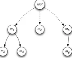
Fernan-Figure 1: Latent tree used for structural learning

des et al. (2014) – render exact inference possi-ble by introducing auxiliary graph structures. The modeling ofFernandes et al. (also referred to as the antecedent tree approach) is exploited in the works ofBj¨orkelund and Kuhn(2014),Martschat and Strube(2015), andLassalle and Denis(2015). Like us, the first couples such approach with ap-proximate inference but for enabling the use of non-local features. The current state-of-the-art model of Wiseman et al. (2016) also employs a greedy inference procedure as it has global fea-tures from an RNN as a non-decomposable term in the inference objective.

3 Structure Output Learning for CR

We consider online learning algorithms for link-ing structured input and output patterns. More formally, such algorithms find a linear mapping

f(x,y) = _hw,Φ(x,y)_i,wheref :X_×Y _→R,

w is a linear model, Φ(x,y) is a combined fea-ture vector of input variables X and output

vari-ablesY. The predicted structure is derived with

theargmax

y∈Y

f(x,y). In the next sections, we show

how to learn w for CR using structured percep-tron. Additionally, we provide a characterization of effective loss functions for separable cases.

3.1 Modeling CR

In this framework, CR is essentially modeled as a clustering problem, where an input-output exam-ple is described by a tuexam-ple(x,y,h),xis a set of entity mentions contained in a text document,yis set of the corresponding mention clusters, and h is a latent variable, i.e., an auxiliary structure that can represent the clusters ofy. For example, given the following text:

Although (she)m1 was supported by (President

Obama)m2, (Mrs. Clinton)m3 missed (her)m4

(chance)m5, (which)m6 looked very good before

counting votes.

Algorithm 1Latent Structured Perceptron

1: Input:X=_{(xi,yi)}ni=1,w0, C, T

2: w_←w0;t←0

3: repeat

4: fori= 1, ..., ndo

5: h∗

i ← argmax h∈H(xi,yi)

hwt,Φ(xi,h)i

6: ˆ_hi←argmax h∈H(xi)

hwt,Φ(xi,h)i+C×∆(yi,h∗i,h)

7: if∆(yi,h∗i,ˆhi)>0then

8: wt+1←wt+ Φ(xi,h∗i)−Φ(xi,hˆi) 9: end if

10: end for

11: t_←t+ 1 12: untilt < nT

13: w← 1

t t

P

i=1

wi

returnw

mentions and the subtrees connected to the addi-tional root node form distinct clusters. The treeh is called a latent variable as it is consistent withy, i.e., it contains only links between mention nodes that corefer or fall into the same cluster according toy. Clearly, an exponential set of trees,H, can

be associated with one and the same clusteringy. Using only one tree to represent a clustering makes the search for optimal mention clusters tractable. In particular, structured prediction algorithms se-lecththat maximizes the model learned at timet

as shown in the next section.

3.2 Latent Structured Perceptron (LSP) The LSP model proposed bySun et al. (2009) and specialized for solving CR tasks byFernandes et al.(2012) is described by Alg.1.

Given a training set {(xi,yi)}ni=1, initial w03,

a trade off parameterC, and the maximum num-ber of epochsT, LSP iterates the following

opera-tions: Line5finds a latent treeh∗_i that maximizes

hwt,Φ(xi,h)ifor the current example(xi,yi). It basically finds the max ground truth tree with re-spect to the current wt. Finding such max re-quires an exploration over the tree setH(xi,yi), which only contains arcs between mentions that corefer according to the gold standard clustering yi. Line6 seeks for the max-violating treeˆhi in

H(xi), which is the set of all candidate trees using

any possible combination of arcs. Line7 tests if the produced tree ˆ_{hi has some mistakes with} re-spect to the gold clusteringyi, using loss function

∆(yi,h∗i,hˆi). Note that some models define a loss exploiting also the current best latent treeh∗_i. If the test is verified, the model is updated with the vectorΦ(xi,h∗i)−Φ(xi,ˆhi).

3_{Either0or a random vector.}

Fernandes et al. (2012) used exactly the di-rected trees we showed as latent structures and applied Edmonds’ spanning tree algorithm ( Ed-monds, 1967) for finding the max. Their model achieved the best results in the CoNLL–2012 Shared Task, a challenge for CR systems ( Prad-han et al.,2012). Their selected loss function also plays an important role as shown in the following.

3.3 Loss functions

When defining a loss, it is very important to pre-serve the factorization of the model components along the latent tree edges since this leads to effi-cient maximization algorithms (see Section5).

Fernandes et al. uses a loss function that (i) compares a predicted tree_hˆ _{against the gold tree} h∗and (ii) factorizes over the edges in the way the model does. Its equation is:

∆F(h∗,ˆh) = M

X

i=1

1_ˆ

h(i)6=h∗(i)(1+r·1h∗_(i)=0),(1)

whereh∗(i)andhˆ(i)output the parent of the

men-tion nodeiin the gold and predicted tree,

respec-tively, whereas1

h∗(i)6=ˆh(i) just checks if the

par-ents are different, and if yes, penalty of1(or1 +r

if the gold parent is the root) is added.

Yu and Joachims’s loss is based on undirected tree without a root and on the gold clusteringy. It is computed as:

∆Y J(y,hˆ) =n(y)−k(y) +

X

e∈ˆ_h

l(y,e), (2)

wheren(y)is the number of graph nodes,k(y)is

the number of clusters iny, andl(y,e)assigns−1

to any edgeethat connects nodes from the same cluster iny, androtherwise.

In our experiments, we adopt both loss func-tions, however, in contrast toFernandes et al., we always measure∆F against the gold labely and not against the currenth∗, i.e., in the way it is done by Martschat and Strube(2015), who employ an equivalent LSP model in their work.

Proposition 1 (Sufficient condition for optimal-ity of loss functions for learning graphs). Let ∆(y,h∗,hˆ) _≥ 0 be a simple, edge-factorizable loss function, which is also monotone in the num-ber of edge errors, and letµ(y,ˆh)be any graph-based measure maximized by no edge errors. Then, if the training set is linearly separable LSP optimizing∆converges to theµoptimum.

Proof. If the data is linearly separable the percep-tron converges ⇒ ∆(yi,h∗i,ˆhi) = 0,∀xi. The loss is factorizable, i.e.,

∆(yi,h∗i,ˆhi) =

X

e∈ˆhi

l(yi,h∗i,e), (3)

where_P l(_·) is an edge loss function. Thus,

e∈hiˆ

l(yi,h∗i,e) = 0. The latter equation and

monotonicity imply l(yi,h∗i,e) = 0,∀e ∈ ˆhi, i.e., there are no edge mistakes, otherwise by fix-ing such edges, we would have a smaller∆, i.e.,

negative, contradicting the initial positiveness hy-pothesis. Thus, no edge mistake in anyxiimplies thatµ(y,ˆh)is maximized on the training set.

Corollary 1. ∆F(h∗,hˆ)and∆Y J(y,ˆh)are both optimal loss functions for graphs.

Proof. Equations 1 and 2 show that both are 0 when applied to a clustering with no mistake on the edges. Additionally, for each edge mis-take more, both loss functions increase, implying monotonicity. Thus, they satisfy all the assump-tions of Proposition1.

The above characteristic suggests that∆F and

∆Y J can optimize any measure that reasonably targets no mistakes as its best outcome. Clearly, this property does not guarantee loss functions to be suitable for a given task measure, e.g., the latter may have different max points and behave rather discontinuously. However, a common practice in NLP is to optimize the maximum of a measure, e.g., in case of Precision and Recall, or Accuracy, therefore, loss functions able to at least achieve such an optimum are preferable.

4 Automatically learning a loss function

How to measure a complex task such as CR has generated a long and controversial discussion in the research community. While such a debate is progressing, the most accepted and used measure is the so-called Mention, Entity, and Link Average (MELA) score. As it will be clear from the de-scription below, MELA is not easily interpretable

and not robust to the mention identification ef-fect (Moosavi and Strube,2016). Thus, loss func-tions showing the optimality property may not be enough to optimize it. Our proposal is to use a version of MELA transformed in a loss function optimized by an LSP algorithm with inexact in-ference. However, the computational complexity of the measure prevents to carry out an effective learning. Our solution is thus to learn MELA with a fast linear regressor, which also produces a con-tinuos version of the measure.

4.1 Measures for CR

MELA is the unweighted average of MUC ( Vi-lain et al.,1995), B3 _{(Bagga and Baldwin,1998)}

and CEAFe(CEAF variant with entity-based sim-ilarity) (Luo,2005;Cai and Strube,2010) scores, having heterogeneous nature.

MUC is based on the number of correctly pre-dicted links between mentions. The number of links required for obtaining the key entity setK

isP_ki∈K(_|ki| −1), wherekiare key entities inK (cardinality of each entity minus one). MUC recall computes what fraction of these were predicted, and the predicted were as many asP_ki∈K(_|ki| −

|p(ki)|) =P_ki∈K(|ki| −1−(|p(ki)| −1)), where

p(ki)is a partition of the key entity ki formed by intersecting it with the corresponding response en-titiesrj ∈R, s.t.,ki∩rj 6=∅. This number equals to the number of the key links minus the number of missing links, required to unite the parts of the partitionp(ki)to obtainki.

B3 _{computes Precision and Recall individually}

for each mention. For mention m: Recallm =

|km i ∩rmj |

|km

i | , where k m

i andrmj , subscripted with m, denote, correspondingly, the key and response en-tities into whichmfalls. The over-document

Re-call is then an average of these taken with respect to the number of the key mentions. The MUC and B3_{Precision is computed by interchanging the}

roles of the key and response entities.

CEAFe computes similarity between key and system entities after finding an optimal alignment between them. Usingψ(ki, rj) = _|2_ki|ki_|+∩_|rj_rj|_| as the entity similarity measure, it finds an optimal one-to-one mapg∗ : K → R,which maps every key

Preci-Algorithm 2 Finding a Max-violating Spanning Tree

1: Input: training example(x,y); graphG(x) with ver-ticesV denoting mentions; set of the incoming candidate edges,E(v),v_∈V; weight vectorw

2: h∗_{← ∅}

3: forv_∈V do

4: e∗= argmax

e∈E(v)h

w,e_i+C_×l(y,e)

5: h∗=h∗_∪e∗

6: end for

7: returnmax-violating treeh∗

8: (clusteringy∗is induced by the treeh∗)

sion and Recall are Ψ(g∗₎ P

rj∈R

ψ(rj,rj) and

Ψ(g∗₎ P

ki∈K

ψ(ki,ki),

respectively.

MELA computation is rather expensive mostly because of CEAFe. Its complexity is bounded by O(M l2logl) (Luo, 2005), where M and l

are, correspondingly, the maximum and minimum number of entities inyandˆy. Computing CEAFe is especially slow for the candidate outputsyˆwith a low quality of prediction, i.e, whenlis big, and

the coherence with the goldyis scarse. Finally, B3 _{and CEAF}

e are strongly influenced by the mention identification effect (Moosavi and Strube, 2016). Thus, ∆F and ∆Y J may output identical values for different clusterings that can have a big gap in terms of MELA.

4.2 Features for learning measures

As computational reasons prevent to use MELA in LSP (see our inexact search algorithm in Sec-tion 5), we study methods for approximating it with a linear regressor. For this purpose, we define nine features, which count either exact or simpli-fied versions of Precision, Recall and F1 of each of the three metric-components of MELA. Clearly, neither∆F nor∆Y J provide the same values.

Apart from the computational complexity, the difficulty of evaluating the quality of the predicted clusteringˆyduring training is also due to the fact that CR is carried out on automatically detected mentions, while it needs to be compared against a gold standard clustering of a gold mention set. However, we can use simple information about au-tomatic mentions and how they relate to gold men-tions and gold clusters. In particular, we use four numbers: (i) correctly detected automatic men-tions, (ii) links they have in the gold standard, (iii) gold mentions, and (iv) gold links. The last one enables the precise computation of Precision, Re-call and F1-measure values of MUC; the required partitionsp(ki)of key entities are also available at

training time as they contain only automatic men-tions. These are the first three features that we de-sign. Likewise for B3_{, the feature values can be} derived using (ii) and (iii).

For computing CEAFe heuristics, we do not perform cluster alignment to find an optimal

Ψ(g∗). Instead of Ψ(g∗), which can be rewrit-ten asP_m∈K∩R 2

|km

i |+|g∗(kim)|if summing up over the mentions not the entities, we simply use_{Ψ =}˜

P

m∈K∩R|km 2

i |+|rmj|, pretending that for each m its keyk_im and response rm_j entities are aligned. P

rj∈Rψ(rj, rj) andPki∈Kψ(ki, ki) in the de-nominators of the Precision and Recall are the number of predicted and gold clusters, corre-spondingly. The imprecision of the CEAFerelated features is expected to be leveraged when put to-gether with the exact B3_{and MUC values into the} regression learning using the exact MELA values (implicitly exact CEAFevalues as well).

4.3 Generating training and test data

The features described above can be used to characterize the clustering variablesyˆ. For gen-erating training data, we collected all the max-violating ˆy produced during LSPF (using ∆F) learning and associate them with their correct MELA scores from the scorer. This way, we can have both training and test data for our regressor. In our experiments, for the generation purpose, we decided to run LSPF on each document separately to obtain more variability inˆy’s. We use a simple linear SVM to learn a modelwρ. Considering that MELA(y,yˆ) score lies in the interval [100,0], a

simple approximation of the loss could be:

∆ρ(y,ˆy) = 100−wρ·φ(y,ˆy). (4) Below, we show its improved version and an LSP for learning with it based on inexact search.

5 Learning with learned loss functions

Our experiments will demonstrate that∆ρ can be accurately learned from data. However, the fea-tures we used for this are not factorizable over the edges of the latent trees. Thus, we design a new LSP algorithm that can use our learned loss in an approximated max search.

Algorithm 3Inexact Inference of a Max-violating Spanning Tree with a Global Loss

1: Input: training example(x,y); graphG(x) with ver-ticesV denoting mentions; set of the incoming candidate

edges,E(v),v∈V;w, ground truth treeh∗

2: ˆ_{h← ∅}

3: score_←0 4: repeat

5: prev score=score

6: score= 0 7: forv_∈V do

8: h=ˆh_\e(v) 9: ˆe= argmax

e∈E(v)h

w,ei+C×∆(y,h∗,h∪e)

10: ˆ_h=h∪ˆe

11: score=score+_hw,ˆe_i

12: end for

13: score=score+ ∆(y,h∗_,ˆ_h)

14: untilscore=prev score

15: returnmax-violating treeˆ_h

inYu and Joachims(2009). The candidate graph, by construction, does not contain cycles, and the inference by Edmonds’ algorithm does technically the same as the ”best-left-link” inference algo-rithm byChang et al.(2012). This can be schemat-ically represented in Alg.2.

When we deal with ∆ρ, Alg. 2 cannot be longer applied as our new loss function is non-factorizable. Thus, we designed a greedy solution, Alg. 3, which still uses the spanning tree algo-rithm, though, it is not guaranteed to deliver the max-violating constraint. However, finding even a suboptimal solution optimizing a more accurate loss function may achieve better performance both in terms of speed and accuracy.

We reformulate Step4of Alg.2, where a max-violating incoming edgeˆeis identified for a ver-texv. The new max-violating inference objective contains now a global loss measured on the par-tial structure _hˆ _{built up to now plus a candidate} edgeefor a vertexvin consideration (Line10of Alg.3). On a high level, this resembles the infer-ence procedure ofWiseman et al.(2016), who use it for optimizing global features coming from an RNN. Differently though, after processing all the vertices, we repeat the procedure until the score of ˆ

hno longer improves.

Note thatBj¨orkelund and Kuhn(2014) perform inexact search on the same latent tree structures to extend the model to non-local features. In contrast to our approach, they use beam search and accu-mulate the early updates.

In addition to the design of an algorithm en-abling the use of our∆ρ, there are other intricacies

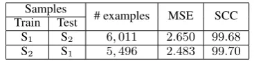
Samples _{# examples MSE SCC} Train Test

S1 S2 6,011 2.650 99.68

S2 S1 5,496 2.483 99.70

Table 1:Accuracy of the loss regressor on two different sets of examples generated from different documents samples.

caused by the lack of factorization that need to be taken into account (see the next section).

5.2 Approaching factorization properties The ∆ρ defined by Equation 4 approximately falls into the interval[0,100]. However, the

sim-ple optimal loss functions, ∆F and ∆Y J, output a value dependent on the size of the input train-ing document in terms of edges (as they factorize in terms of edges). Since this property cannot be learned from MELA by our regression algorithm, we calibrate our loss with respect to the number of correctly predicted mentions,c, in that document,

obtaining∆0_ρ= ₁₀₀c ∆ρ.

Finally, another important issue is connected to the fact that on the way as we incrementally con-struct a max-violating tree according to Alg.3,∆ρ decreases (and MELA grows), as we add more mentions to the output, traversing the tree nodes v. Thus, to equalize the contribution of the loss among the candidate edges of different nodes, we also scale the loss of the candidate edges of the node v having order i in the document,

accord-ing to the formula ∆00_ρ = _|Vi_|∆0_ρ. This can be

interpreted as giving more weight to the hard-to-classify instances – an important issue alleviated by Zhao and Ng (2010). Towards the end of the document, the probability of correctly predicting an incoming edge for a node generally decreases, as increases the number of hypotheses.

6 Experiments

In our experiments, we first show that our re-gressor for learning MELA approximates it rather accurately. Then, we examine the impact of our

∆ρon state-of-the-art systems in comparison with other loss functions. Finally, we show that the im-pact of our model is amplified when learning in smaller feature spaces.

6.1 Setup

Data We conducted our experiments on En-glish and Arabic parts of the corpus from CoNLL 2012-Shared Task4_{. The English data contains}

2,802, 343, and 348 documents in the training,

101 ₁₀2 ₁₀3 2

4 6 8 10 12

number of training examples

MSE

101 ₁₀2 ₁₀3

98.8

99.0

99.2

99.4

99.6

99.8

number of training examples

SCC

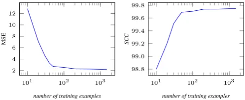
Figure 2:Regressor Learning curves.

dev. and test parts, respectively. The Arabic data includes 359, 44, and 44 documents for training, dev. and test sets, respectively.

Models We implement our version of LSP, where LSPF, LSPY J, and LSPρuse the loss func-tions, ∆F, ∆Y J, and ∆ρ, defined in Section3.3 and 5.2, respectively. We used cort5 _–

coref-erence toolkit by Martschat and Strube (2015) both to preprocess the English data and to extract candidate mentions and features (the basic set). For Arabic, we used mentions and features from BART6 _{(Uryupina et al.,2012). We extended the}

initial feature set for Arabic with the feature com-binations proposed by Durrett and Klein (2013), those permitted by the available initial features. Parametrization All the perceptron models re-quire tuning of a regularization parameter C.

LSPF and LSPY J – also tuning of a specific loss parameter r. We select the parameters on

the entire dev. set by training on 100 random

documents from the training set. We pick up

C ∈ {1.0,100.0,1000.0,2000.0}, the r

val-ues for LSPF from the interval [0.5,2.5] with step 0.5, and the r values for LSPY J – from

{0.05,0.1,0.5}. Ultimately, for English, we used

C = 1000.0in all the models; r = 1.0 in LSPF andr = 0.1in LSPY J. And wider ranges of pa-rameter values were considered for Arabic, due to the lower mention detection rate: C = 1000.0,

r = 6.0 for LSPF, C = 1000.0, r = 0.01 for LSPY J, andC = 5000.0– for LSPρ. A standard previous work setting for the number of epochsT

of LSP is5(Martschat and Strube,2015). Fernan-des et al.(2014) noted thatT = 50was sufficient

for convergence. We selected the bestT from1to 50on the dev. set.

Evaluation measure We used MUC, B3_{, CEAF}

e and their average MELA for evaluation, computed by the version 8 of the official CoNLL scorer.

5_{http://smartschat.de/software} 6_{http://www.bart-coref.org/}

Model Selected_{Dev. Test}(N= 1_TM) All(N∼16.8M) best Dev. Test Tbest LSPF 63.72 62.19 49 64.05 63.05 41 LSPY J 63.72 62.44 29 64.32 62.76 13 LSPρ 64.12 63.09 27 64.30 63.37 18 M&S AT – – – 62.31 61.24 5 M&S MR – – – 63.52 62.47 5 B&K – – – 62.52 61.63 – Fer – – – 60.57 60.65 –

Table 2:Results of our and previous work models evaluated on the dev. and test sets following the exact CoNLL-2012 En-glish setting, using all training documents with All and1M

features.Tbestis evaluated on the dev. set. 6.2 Learning loss functions

For learning MELA, we generated training and test examples from LSPF according to the proce-dure described in Section4.3. In the first experi-ment, we trained thewρmodel on a set of exam-ples S1, generated from a sample of100English

documents and tested on a set of examples S2,

gen-erated from another sample of the same size, and vice versa. The results in Table1show that with just5,000/6,000, the Mean Squared Error (MSE)

is roughly between∼ 2.4₋2.7: these are rather

small numbers considering that the regression out-put values in the interval [0,100]. Squared

Cor-relation Coefficient (SCC) reaches a corCor-relation of about 99.7%, demonstrating that our regression approach is effective in estimating MELA.

Additionally, Figure 2 shows the regression learning curves evaluated with MSE and SCC. The former rapidly decreases and, with about 1,000

examples, reaches a plateau of around2.3. The

lat-ter shows a similar behaviour, approaching a cor-relation of about 99.8% with real MELA.

6.3 State of the art and model comparison We first experimented with the standard CoNLL setting to compare the LSP accuracy in terms of MELA using the three different loss functions, i.e., LSPF, LSPY J and LSPρ. In particular, we used all the documents of the training set and all

N ∼16.8M features from cort, and tested on the

both dev. and test sets. The results are reported in Columns All of Table2.

We note first that our∆ρis effective as it stays on a par with∆F and∆Y J on the dev. set. This is interesting as Corollary1shows that such func-tions can optimize MELA, the reported values re-fer to the optimal epoch numbers. Also, LSPρ im-proves the other models on the test set by0.3

per-cent points (statistical significant at the93%level

0 25 50 75 100 42

44 46 48

number of epochs,T

MELA

N= 10K

0 25 50 75 100

54 56 58 60

number of epochs,T

MELA

N= 100K

0 25 50 75 100

56 58 60 62

number of epochs,T

MELA

N= 300K

0 25 50 75 100

58 60 62 64

number of epochs,T

MELA

N= 500K

0 25 50 75 100

60 62 64

number of epochs,T

MELA

N= 1M

0 25 50 75 100

60 62 64

number of epochs,T

MELA

N= 1.5M

0 25 50 75 100

61 62 63 64

number of epochs,T

MELA

All (N∼16.8M)

104 105 106 107

45 50 55 60 65

number of features,N

M

E

LA

All on the Test Set

LSPF LSPY J LSPρ

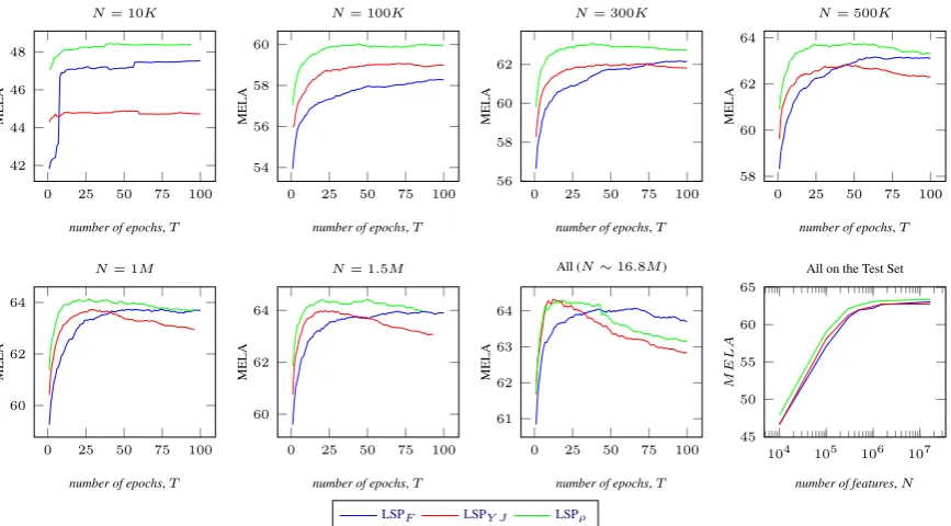
Figure 3:Results of LSP models on the dev. set using different number of features,N. The last plot reports MELA score on the test set of the models using the optimal number of epochs tuned on the dev. set.

#Feat. Model Test Set

M U C B3 CEAFe M ELA

All LSPF 72.66 59.94 56.54 63.05 LSPY J 72.18 59.31 55.82 62.76 LSPρ 72.34 60.36 57.40 63.37 LSPF 71.95 59.03 55.59 62.19 1M LSPY J 72.35 59.54 56.38 62.44 LSPρ 72.09 60.11 57.07 63.09 Table 3: Results on the test set using the same setting of Table2and the measures composing MELA.

Secondly, all the three models improve the state of the art on CR using LSP, i.e., by Martschat and Strube (2015) using antecedent trees (M&S AT) or mention ranking (M&S MR), Bj¨orkelund and Kuhn (2014) using a global feature model (B&K) and Fernandes et al.(2014) (Fer). Noted that all the LSP models were trained on the train-ing set only, without retraintrain-ing on the traintrain-ing and dev. sets together, thus our scores can be improved. Thirdly, Table 3 shows the breakdown of the MELA results in terms of its components on the test set. Interestingly, LSPρis noticeably better in terms of B3 _{and CEAF}

e, while LSP with simple losses, as expected, deliver higher MUC score.

Finally, the overall improvement of ∆ρ is not impressive. This mainly depends on the optimal-ity of the competing loss functions, which in a set-ting of∼ 16.8M features, satisfy the separability

condition of Proposition1.

6.4 Learning in more challenging conditions In these experiments, we verify the hypothesis that when the optimality property is partially or

totally missing∆ρis more visibly superior to∆F and∆Y J. As we do not want to degrade their ef-fectiveness, the only condition dependent on the setting is the data inseparability or at least harder to be separated. These conditions can be obtained by reducing the size of the feature space. How-ever, since we aim at testing conditions, where∆ρ is practically useful, we filter out less important features, preserving the model accuracy (at least when the selection is not extremely harsh). For this purpose, we use a feature selection approach using a basic binary classifier trained to discrimi-nate between correct and incorrect mention pairs. It is typically used in non structured CR methods and has a nice property of using the same fea-tures of LSP (we do not use global feafea-tures in our study). We carried out a selection using the abso-lute values of the model weights of the classifier for ranking features and then selecting those hav-ing higher rank (Haponchyk and Moschitti,2017). The MELA produced by our models using all the training data is presented in Figure 3. The first 7 plots show learning curves in terms of LSP epochs for different feature sets with increasing size N, evaluated on the dev. set. We note that:

sep-arable) thus a loss function which is closer to the real measure provides some advantages.

Secondly, when using all features, LSPρis still overall better than the other models but clearly the latter can achieve the same MELA on the dev. set. Thirdly, the last plot shows the MELA produced by LSP models on the test set, when trained with the best epoch derived from the dev. set (previous plots). We observe that LSPρ is constantly better than the other models, though decreasing its effect as the feature number increases.

Next, in Column 1 (Selected) of Table 2, we report the model MELA using 1 million features. We note that LSPρ improves the other models by at least 0.6 percent points, achieving the same ac-curacy as the best of its competitors, i.e., LSPF, using all the features.

Finally, ∆ρ does not satisfy Proposition 1, therefore, generally, we do not know if it can op-timize any µ-type measure over graphs.

How-ever, being learned to optimize MELA, it clearly separates data maximizing such a measure. We empirically verified this by checking the MELA score obtained on the training set: we found that LSPρalways optimizes MELA, iterating for fewer epochs than the other loss functions.

6.5 Generalization to other languages

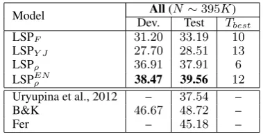
Here, we test the effectiveness of the proposed method on Arabic using all available data and fea-tures. The results in Table4reveal an indisputable superiority of LSPρover the counterparts optimiz-ing simple loss functions. They support the results of the previous section as we had to deal with the insufficiency of the expert-based features for Ara-bic. In such an uneasy case, LSPρwas able to im-prove over LSPF by more than 4.7 points.

We also tested the loss model wρ trained for the experiments on the English data (resp. setting All of Section6.3) in LSPρ on Arabic. This cor-responds to LSPEN

ρ model. Notably, it performs even better, 1.5 points more, than LSPρ using a loss learned from Arabic examples. This suggests a nice property of data invariance of∆ρ. The im-provement delivered by the ”English” wρ is due to the fact that it was trained on the data which is richer: (i) quantitatively, since coming from al-most 8 times more training documents in compar-ison to Arabic and (ii) qualitatively, in a sense of diversity with respect to the RL target value. In-deed, the Arabic data is much less separable than

Model _Dev.All(N_Test∼395K_T) best

LSPF 31.20 33.19 10

LSPY J 27.70 28.51 13

LSPρ 36.91 37.91 6

LSPEN

ρ 38.47 39.56 12 Uryupina et al., 2012 – 37.54 – B&K 46.67 48.72 –

Fer – 45.18 –

Table 4: Results of our and baseline models evaluated on the dev. and test sets following the exact CoNLL-2012 Arabic setting, using all training documents. Tbestis evaluated on the dev. set.

the English data and this prevents to have exam-ples where MELA values are higher.

7 Conclusions

In this paper, we studied the use of complex loss functions in structured prediction for CR. Given the scale of our investigation, we limited our study to LSP, which is anyway considered state of the art. We derived several findings: (i) for the first time, up to our knowledge, we showed that a com-plex measure, such as MELA, can be learned by a linear regressor (RL) with high accuracy and ef-fective generalization. (ii) The latter was essential for designing a new LSP based on inexact search and RL. (iii) We showed that an automatically learned loss can be optimized and provides state-of-the-art performance in a real setting, including thousands of documents and millions of features, such as CoNLL–2012 Shared Task. (iv) We de-fined a property of optimal loss functions for CR, which shows that in separable cases, such losses are enough to get the state of the art. However, as soon as separability becomes more complex sim-ple loss functions lose optimality and RL becomes more accurate and faster. (v) Our MELA approxi-mation provides a loss that is data invariant which, once learned, can be optimized in LSP on different datasets and in different languages.

Our study opens several future directions, rang-ing from definrang-ing algorithms based on automati-cally learned loss functions to learning more ef-fective measures from expert examples.

Acknowledgements

References

Amit Bagga and Breck Baldwin. 1998. Algorithms for scoring coreference chains. In Proceedings of the Linguistic Coreference Workshop at the First In-ternational Conference on Language Resources and Evaluation. Granada, Spain, pages 563–566.

Anders Bj¨orkelund and Jonas Kuhn. 2014. Learn-ing structured perceptrons for coreference resolu-tion with latent antecedents and non-local features. In Proceedings of the 52nd Annual Meeting of the Association for Computational Linguistics (Volume 1: Long Papers). Association for Computational Linguistics, Baltimore, Maryland, pages 47–57.

http://www.aclweb.org/anthology/P/P14/P14-1005.

Jie Cai and Michael Strube. 2010. Evaluation metrics for end-to-end coreference resolution systems. In Proceedings of the 11th Annual Meeting of the Special Interest Group on Discourse and Dia-logue. Association for Computational Linguistics, Stroudsburg, PA, USA, SIGDIAL ’10, pages 28–36.

http://dl.acm.org/citation.cfm?id=1944506.1944511.

Kai-Wei Chang, Rajhans Samdani, Alla Rozovskaya, Mark Sammons, and Dan Roth. 2012. Illinois-coref: The ui system in the conll-2012 shared task. In Joint Conference on EMNLP and CoNLL - Shared Task. Association for Computa-tional Linguistics, Jeju Island, Korea, pages 113– 117. http://www.aclweb.org/anthology/W12-4513.

Kevin Clark and Christopher D. Manning. 2016. Im-proving coreference resolution by learning entity-level distributed representations. In Proceed-ings of the 54th Annual Meeting of the As-sociation for Computational Linguistics (Volume 1: Long Papers). Association for Computational Linguistics, Berlin, Germany, pages 643–653.

http://www.aclweb.org/anthology/P16-1061.

Greg Durrett and Dan Klein. 2013. Easy victories and uphill battles in coreference resolution. InIn Pro-ceedings of the 2013 Conference on Empirical Meth-ods in Natural Language Processing.

Jack Edmonds. 1967. Optimum branchings. Journal of research of National Bureau of standardspages 233–240.

Eraldo Rezende Fernandes, C´ıcero Nogueira dos Santos, and Ruy Luiz Milidi´u. 2012. Latent structure perceptron with feature induction for unrestricted coreference resolution. In Joint Conference on EMNLP and CoNLL -Shared Task. Association for Computational Linguistics, Jeju Island, Korea, pages 41–48.

http://www.aclweb.org/anthology/W12-4502.

Eraldo Rezende Fernandes, C´ıcero Nogueira dos San-tos, and Ruy Luiz Milidi´u. 2014. Latent trees for coreference resolution. Computational Linguistics 40(4):801–835.

Thomas Finley and Thorsten Joachims. 2005.

Supervised clustering with support vector ma-chines. In ICML ’05: Proceedings of the 22nd international conference on Machine learning. ACM, New York, NY, USA, pages 217–224.

https://doi.org/10.1145/1102351.1102379.

Iryna Haponchyk and Alessandro Moschitti. 2017. A practical perspective on latent structured predic-tion for coreference resolupredic-tion. In Proceedings of the 15th Conference of the European Chapter of the Association for Computational Linguistics: Volume 2, Short Papers. Association for Computa-tional Linguistics, Valencia, Spain, pages 143–149.

http://www.aclweb.org/anthology/E17-2023. Emmanuel Lassalle and Pascal Denis. 2015.

Joint anaphoricity detection and corefer-ence resolution with constrained latent struc-tures. In Proceedings of the Twenty-Ninth AAAI Conference on Artificial Intelligence. AAAI Press, AAAI’15, pages 2274–2280.

http://dl.acm.org/citation.cfm?id=2886521.2886637. Xiaoqiang Luo. 2005. On coreference resolution

per-formance metrics. In Proceedings of the Con-ference on Human Language Technology and Em-pirical Methods in Natural Language Process-ing. Association for Computational Linguistics, Stroudsburg, PA, USA, HLT ’05, pages 25–32.

https://doi.org/10.3115/1220575.1220579.

Sebastian Martschat and Michael Strube. 2015. La-tent structures for coreference resolution. Transac-tions of the Association for Computational Linguis-tics3:405–418.

Nafise Sadat Moosavi and Michael Strube. 2016.

Which coreference evaluation metric do you trust? a proposal for a link-based entity aware metric. In Proceedings of the 54th Annual Meeting of the Association for Computational Linguistics (Vol-ume 1: Long Papers). Association for Computa-tional Linguistics, Berlin, Germany, pages 632–642.

http://www.aclweb.org/anthology/P16-1060. Sameer Pradhan, Alessandro Moschitti,

Nian-wen Xue, Olga Uryupina, and Yuchen Zhang. 2012. Conll-2012 shared task: Modeling mul-tilingual unrestricted coreference in ontonotes. In Joint Conference on EMNLP and CoNLL - Shared Task. Association for Computational Linguistics, Jeju Island, Korea, page 1–40.

http://www.aclweb.org/anthology/W12-4501. Xu Sun, Takuya Matsuzaki, Daisuke Okanohara,

and Jun’ichi Tsujii. 2009. Latent variable perceptron algorithm for structured classifi-cation. In Proceedings of the 21st Interna-tional Jont Conference on Artifical Intelligence. Morgan Kaufmann Publishers Inc., San Fran-cisco, CA, USA, IJCAI’09, pages 1236–1242.

http://dl.acm.org/citation.cfm?id=1661445.1661643. Olga Uryupina, Alessandro Moschitti, and

The unitn/essex submission to the conll-2012 shared task. In Joint Conference on EMNLP and CoNLL - Shared Task. Associa-tion for ComputaAssocia-tional Linguistics, Strouds-burg, PA, USA, CoNLL ’12, pages 122–128.

http://dl.acm.org/citation.cfm?id=2391181.2391198.

Olga Uryupina, Sriparna Saha, Asif Ekbal, and Massimo Poesio. 2011. Multi-metric optimization for coreference: The unitn/iitp/essex submission to the 2011 conll shared task. In Proceedings of the Fifteenth Conference on Computational Natural Language Learning: Shared Task. Associ-ation for ComputAssoci-ational Linguistics, Stroudsburg, PA, USA, CONLL Shared Task ’11, pages 61–65.

http://dl.acm.org/citation.cfm?id=2132936.2132944.

Marc Vilain, John Burger, John Aberdeen, Dennis Con-nolly, and Lynette Hirschman. 1995. A model-theoretic coreference scoring scheme. In Proceed-ings of the 6th Message Understanding Conference. pages 45–52.

Sam Wiseman, Alexander M. Rush, and Stuart M. Shieber. 2016. Learning global features for coref-erence resolution. In NAACL HLT 2016, The 2016 Conference of the North American Chapter of the Association for Computational Linguistics: Human Language Technologies, San Diego Cali-fornia, USA, June 12-17, 2016. pages 994–1004.

http://aclweb.org/anthology/N/N16/N16-1114.pdf.

Chun-Nam John Yu and Thorsten Joachims. 2009.

Learning structural svms with latent variables. In Proceedings of the 26th Annual International Conference on Machine Learning. ACM, New York, NY, USA, ICML ’09, pages 1169–1176.

https://doi.org/10.1145/1553374.1553523.