Long run expectations in a Learning to Forecast Experiment: a simulation approach

Munich Personal RePEc Archive

Long-run expectations in a

Learning-to-Forecast-Experiment: a

simulation approach

Colasante, Annarita and Alfarano, Simone and Camacho

Cuena, Eva and Gallegati, Mauro

Universitat Jaume I, Spain, Universitat Jaume I, Spain, Universitat

Jaume I, Spain, Università Politecnica delle Marche, Italy

Long-run expectations in a Learning-to-Forecast

Experiment: A Simulation Approach

Annarita Colasante

, Simone Alfarano

, Eva Camacho Cuena

, Mauro Gallegati

1

_{University Jaume I (Spain),}

_{Universit`a Politecnica delle Marche(Italy)}

Abstract

In this paper, we elicit both short and long-run expectations about the evolution of the price of a financial asset by conducting a Learning-to-Forecast Experiment (LtFE) in which subjects, in each period, forecast the the asset price for each one of the remaining periods. The aim of this paper is twofold: on the one hand, we try to fill the gap in the experimental literature of LtFEs where great effort has been made in investigating short-run expectations, i.e. one step-ahead predictions, while there are no contributions that elicit long-run expec-tations. On the other hand, we propose an alternative computational approach with respect to the Heuristic Switching Model (HSM), to replicate the main experimental results. The al-ternative learning algorithm, called Exploration-Exploitation Algorithm (EEA), is based on the idea that agents anchor their expectations around the last market price, rather than on the fundamental value, with a range proportional to the recent past observed price volatility. Both algorithms perform well in describing the dynamics of short-run expectations and the market price. EEA, additionally, provides a fairly good description of long-run expectations.

JEL:D03 G12 C91

Keywords:Expectations, Experiment, Evolutionary Learning

1

Introduction

The economy can be formally thought as an expectation feedback system, i.e. a system where agents’ expectations, formed based on available information and on past realizations of economic variables, influence future realizations of those variables Hommes [2001]. The comprehension of how individual agents form their expectations constitutes a crucial aspect, on the one hand, for understanding the evolution of the economic system itself and, on the other hand, in devising efficient economic policies to guide it towards social desirable outcomes. One of the main prob-lems when dealing with expectations is that they are not directly observable, contrary to prices, volumes, interest rates and all economic variables recorded every day in world-wide markets. There are several cleverly designed methods to directly or indirectly estimate agents’ expecta-tions based on surveys (for a overview see Manski [2004]). However surveys do not typically provide incentives depending on the performance of the responders, so their validity turns out to be limited.

to Forecasts Experiments, introduced by Marimon et al. [1993], are laboratory control experi-ments to elicit subjects’ expectations in an expectation-feedback environment, where the feedback between the subjects’ expectations and the aggregate quantities, typically prices, is designed by the experimenter. They turn out to be a powerful and flexible tool to study subjects’ expec-tation formation under different feedback systems. Many LtFEs have been conducted to study how agents form their short-run expectations in financial markets (Hommes et al. [2005]), real estate markets (Bao and Ding [2015]), commodity markets (Bao et al. [2013]) and in simple macroeconomic frameworks (Assenzaa et al. [2011], Anufriev et al. [2013a], Cornand et al. [2013]). We conduct a Learning to Forecast Experiment (LtFE) in which, unlike the standard settings1

, subjects should submit a prediction for the asset price at different time horizons. In other words, we explicitly elicit subjects’ long-run expectations at the beginning of every period, giving the possibility to revise their expectations as new information becomes available. The novelty of our experimental design is that it incorporates into the LtFEs the elicitation of long-run ex-pectations, in order to study how expectations form and co-evolve with the market price. Our setting is extremely simple, since long-run expectations do not enter directly in the feedback mechanism, which is influenced just by one-step-ahead predictions.2 _{Therefore, we can study}

how subjects form their long-run expectations based solely on price dynamics. We consider our setting a first step in the direction of a better understanding of the dynamics of expectations in more complex environments. With our paper, we want to fill the gap in the existing experimental literature in eliciting the whole spectrum of subjects’ individual expectations. To the best of our knowledge, the only experimental work that elicit the long-run expectations in an asset market with bubbles is the work of Haruvy et al. [2007]. Moreover, Hanaki et al. [2016] investigate the impact of forecast elicitation on the miss-pricing in an experimental asset market. A kind of natural experiment has been conducted by Galati et al. [2011] , where they elicit short, medium and long-run inflation expectations using professional forecasters from central banks, academics and students. They provide, when possible, a reward based on the performances. Some effort has been devoted to elicit long-run expectations using data from surveys (Ashiya [2003], Fujiwara et al. [2013]), but they are not immune to the critical aspects related to the survey methodology. Why are we interested in eliciting long-run expectations? Several empirical as well as theoret-ical contributions have stressed the importance of taking into account the whole time spectrum of agents’ expectations when designing effective economic policies (Gurkaynak et al. [2005], Cœur´e [2013]). Since early 2000s, Central Banks follow a “forward guidance” communication strategy (Woodford [2001]) to try to influence expectations by releasing public announcements on differ-ent macroeconomic indicators. Cdiffer-entral Banks might also establish medium-term inflation target, to discipline the expectations of economic actors. In both cases, Central -Banks, when devising their monetary policy, take into consideration agents’ expectations at different time horizons. These are just examples of why understanding the way agents form and revise their expectations at different time horizons is a relevant issue for policy design.

In the second part of the paper we introduce a learning algorithm able to reproduce the properties of the short as well as long-run expectations observed in our experiment. In the literature of LtFE we find several computational attempts to describe short-run expectations in different experimental settings and information sets using learning algorithms to simulate human behavior. For example, LtFEs with positive and negative feedback, with exogenous shocks, or in a macroeconomic environment as in Heemeijer et al. [2009], Assenzaa et al. [2011], Bao et al. [2013], Hommes and Lux [2013]. A unified framework has been proposed with the aim of reproducing

1

For a comprehensive survey on the macroeconomic experiments on expectations see Assenza et al. [2014]

2

all experimental results od LtFEs, the so-called Heuristic Switching Model. This approach is based on the idea that each subject considers a limited number of simple extrapolative rules (heuristics), based on the seminal paper of Brock and Hommes [1998]. The artificial agents can switch heuristic depending on the forecasting performance in the recent past. The learning mechanism is based on a performance measure proportional to the quadratic forecasting error (see for example Anufriev and Hommes [2012]).

We propose an alternative approach to HSM to model individual behavior in a LtFE. We introduce an algorithm that we can loosely define as “non-parametric” since it does not impose any predetermined forecasting rule. The main idea arises from the analysis based on professional forecasters as in Campbell and Sharpe [2009] and Nakazono [2012]). According to these studies, professional forecasters, in order to reduce the uncertainty about the future, use the last observed price as an anchor. Looking at the experimental results in LtFEs, especially in the one step-ahead predictions, subjects predict the next price anchoring their predictions around the last realized price. A similar mechanism holds for the long-run predictions, as shown in Colasante et al. [2016]. The alternative algorithm proposed in this paper, called the Exploration-Exploitation Algorithm, is based on the empirical as well as experimental evidence that agents anchor their expectations around the last market price conditioning the range of variability of expectations on the past observed price volatility. The EEA is similar to those algorithms used to solve the multi-armed bandit problem (see Auer et al. [2002] and Koulouriotis and Xanthopoulos [2008]). In this kind of computational problems artificial agents face a trade-off betweenexploitationandexploration, i.e. taking a decision using “known and cheap” information up to period t or gathering “new and costly” information about the environment by exploring the “neighbourhood space”.

All in all, the HSM and EEA are based on the well-known behavioral principle of anchor-and-adjustment, with the difference that the HSM has a predetermined set of few rules, while the EEA has a wider set of variability of the feasible actions available to the agents3

. We show that EEA and HSM perform well in describing the dynamics of short-run expectations and the market price. EEA additionally provides a fairly good description of long-term expectations, contrary to benchmark version of current version HSM, which is structurally designed to describe short-term expectations.

2

The Learning to Forecast Experiment

2.1

Experimental Design

Our goal is to study expectations formation both, in the short and in the long-run. We implement a LtFE similar to Heemeijer et al. [2009], where the task of subjects is to predict the future price of an asset. In each of the 7 sessions implemented, 6 subjects play the role of professional forecasters for 20 periods (see the instructions in the complementary material). At the beginning of periodt, subjectisubmits her short-run prediction for the asset price at the end of periodt, denoted asipet,t, as well as her set of long-run predictions for the price at the end of each one of

the 20−t remaining periods. Long-run predictions are denoted as ipet,t+kwith 1 ≤k ≤20−t.

Subjects must submit a total of 190 predictions, since we elicit contemporaneously both short and long-run predictions. The choice of 20 periods, contrary to the approximately 50 one-step-ahead predictions typically used in the literature, results from a trade-off between having a time series sufficiently long to conduct a meaningful statistical analysis and, at the same time, avoid

3

a too demanding task to the subjects.4

When submitting their predictions, subjects are informed about: (i) the constant interest rate (r) and average dividend (d), (ii) the asset prices until periodt−1, (iii) all their own (short and long-run) past predictions and their corresponding profits. However, they are not informed about the predictions submitted by the other subjects and have just qualitative information on the price generating mechanism. In the instructions subjects are informed that there is a positive relationship between their one-step-ahead predictions and the next realized price. We provide in the appendix a screen shot of the experiment and the translated instructions in the supplementary material.

We follow the approach of Heemeijer et al. [2009] in deriving the pricing equation. The function connecting the prediction and the price is the following:

pt=pf+

1 1 +r(¯p

e

t,t−pf) +ǫt (1)

where r= 0.05 in all sessions and d is equal to 3.5 or 3.25 depending on the session. The fundamental price is computed aspf =d_r. ¯pet,tis the average of the six one-step-ahead predictions

submitted at the beginning of periodtp¯e t,t=

1 6

P6

i=1ipet,t, and the termǫt∼N(0,0.25) is an iid

Normal shock. Looking at eq. (1), there is a strong positive feedback between expectations and market price, according to Hommes [2013].

Individual earnings at the end of each period depend on both, short and long-run prediction errors and are computed asiπt=iπst+iπlt. We denote asiπst the subject pay-off that depends

on her short-run prediction error:

iπts=

250

1 +β with β=

ipet,t−pt

2

2

(2)

and as iπtl the subject pay-off that depends on long-run prediction error. We define iπtl =

Pt−1

j=1 iπ

l

t−j,t, whereiπ

l

t−j,t represents the individual profit associated with the accuracy of the

prediction submitted by subjectiat the beginning of periodt−jabout the asset price in period

t, where 1≤j≤t−1. It is computed according to the following payment schedule:5

iπlt₋j,t=

     

    

25 if 0≤iδt₋j,t≤5

12 if 5<iδt−j,t≤10

5 if 10<iδt₋j,t≤15

0 otherwise

where iδt−j,t = |ip

e

t₋j,t−pt|. The final payment of each subject is the sum of pay-offs across

all periods. We calibrated the parameters of the pay-off functions such that approximately maxP20

t=1iπts = max

P20

t=1iπlt, in order to give to the subjects the same incentive to provide

accurate predictions in the short as well as in the long-run. Note that subjects have an immediate feedback about the accuracy of their short-run predictions, while they experience a delay in evaluating the accuracy of their long-run predictions.

4

It is important to underline that subjects attention do not decrease over time. To stress this aspect, we compute the average time taken by subjects to submit their predictions. Subjects take about 3 minutes to submit 20 predictions in the first period, and, at the end of the session, they take on average 40 seconds to submit just one predictions. We claim that each prediction, from the first to the last period, is a reasoned choice and it is not the result of an hasty choice.

5

The experiment involves 42 undergraduate students and it was conducted in the Laboratory of Experimental Economics at University Jaume I. Each session lasted approximatively 40 minutes and the average gain was 20 Euros.

We can compute the Rational Expectations Equilibrium (Lucas Jr [1978]) of our experiment. According to the law of motion of eq. (1), the REE implies that the realized price pt should

converge to the fundamental value with very small fluctuations due to the idiosyncratic shock

ǫt. If we assume all subjects have rational expectations, their predictions6 in each periodt and

for each forecasting horizon kshould fluctuate around the constant fundamental value, i.e.

ipet,t+k ≈pf. This condition can be easily tested using our experimental data. It might be that

the price as well as short-run expectations converge to the fundamental value, a case observed in the literature, however long-run expectations do not. This scenario is, in principle, not in line with REE in our setting with constant fundamental value. On the other hand, it might be that long-run expectations converge to the fundamental value, while the short-run ones together with the price dynamics do not. This hypothetical scenario would signal that subjects would consider the fundamental value as a kind of asymptotic equilibrium. Our experimental design allows to measure whether and how the price dynamics together with entire spectrum of expectations, short and long-run, converges to the fundamental value.

Note that in the eq. (1) we explicitly exclude the dependence of the price on long-run expectations. This allows us for a direct comparison of our results with the outcome of other LtFEs present in the literature. In principle, one might expect that, since long-run expectations do not enter in the price generating equation, they do not significantly impact the price dynamics. However, since subjects’ pay-off does depend on the accuracy of their long-run expectations, we cannot excludea priori that subjects use long-run expectations for some kind of inter-temporal hedging, influencing therefore the price dynamics. In this case, in fact, short-run predictions should be influenced by past long-run predictions. In this paper, we will show that such effect, if it exits, has a negligible impact on the price dynamics. Therefore, short-run expectations are independent of the elicitation of long-run expectations. In particular, we can study how past price dynamics is incorporated into the subjects’ short-run expectations and whether and how short-run expectations and the past time series of prices influence long-run expectations. Do short- and long-run expectations follow the same pattern? If subjects learn to coordinate their short-run expectations, as shown in the learning to forecast literature, how their long-run expectations behave? Do they coordinate? Do they converge to the asset fundamental value?

2.2

Experimental results

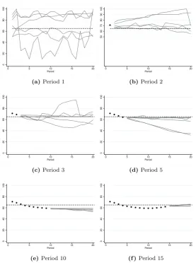
Figure 1 shows individual short-run predictions and realized market prices for all groups. In the Appendix, Figures from 21 to 27 describe individual long-run predictions as well as the evolution of the market price for the 20 periods and for all 7 groups. As an example, Figure 2 shows the evolution over time of the market price together with individual long-run predictions of one of the groups.

From a visual inspection of those Figures, we observe two interesting regularities. The first regularity is an apparent pivotal role of the last realized price in the formation of expectations. This effect is particularly evident if we compare the whole set of expectations submitted in the first period, when subjects have no price available, to those submitted in period 2 (see panels (a) and (b) in Figures from 21 to 27 in the Appendix). In particular, the pivotal effect of the last realized price on the expectations’ dynamics can be clearly identified if one considers the strong reduction in the heterogeneity of the entire spectrum of expectations submitted in the second period with respect to the first one; such reduction persists for several of the subsequent

6

periods. The second interesting feature is that subjects’ long-run expectations are persistently heterogeneous across periods and the heterogeneity appears to increase with the time horizon. An important question arises: Which is the origin of such heterogeneity? We are sure that it cannot be a difference in the subjects’ information set, since the past price dynamics is com-mon and comcom-mon knowledge acom-mong subjects. We can conjecture that subjects have different

interpretations of whether and how past prices influence future prices. In this respect, our ex-perimental design allows to better measure the heterogeneity in the way individual subjects form their expectations using their available information as compared to other LtFEs in the literature, that are typically limited to one-period-ahead predictions, since we have a more comprehensive measures of their expectations.

2.2.1 Coordination of short and long-run expectations

Given the strong positive feedback between the short-run predictions and market prices from eq. (1), each subject has to guestimate the expectations of the other subjects when submitting her short-run predictions. It exists, in fact, a strategic interaction among subjects: each subject has an incentive to coordinate her expectations around the others’ expectations: subjects’ ex-pectations are strategic complements. We, therefore, expect a strong coordination of subjects’ short-run predictions, in line with the literature (see for example Heemeijer et al. [2009]). What about long-run predictions? Whereas subjects have a direct incentive to coordinate their short-run expectations, their coordination motive for long-short-run expectations is more complex. When submitting their long-run predictions, the subject’s task is to forecast at the beginning of period

tthe price at the end of periodt+k, withk >0. The price at the end of periodt+kdepends on the subjects’ short-run predictions submitted at the beginning of period t+k. Therefore they should guestimate,k-periods in advance, the short-run expectations of the other subjects at the beginning of periodt+k. We should expect, then, a lower degree of coordination the longer is the forecasting horizon, given the increasingly degree of uncertainty in guestimating the future short-run behavior of the other subjects.

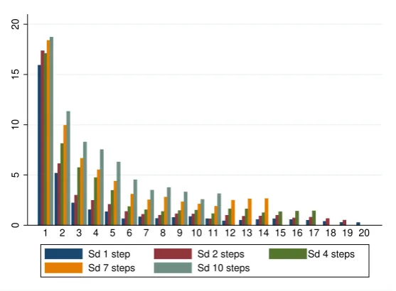
In order to measure the degree of coordination of subjects’ expectations, we compute the standard deviation of their predictions submitted at a given period and for different time hori-zons. Figure 3 shows the average standard deviation of subjects’ predictions submitted in period

t for the price at the end of period t+k. In line with the LtFEs literature, we observe a fast coordination of subjects’ short-run predictions. The heterogeneity of subjects’ short-run pre-dictions declines rapidly during the first 5 periods, to reach afterwards an almost stable value. Also for long-run predictions the degree of coordination increases over time. However, long-run expectations clearly need more time to reach the same coordination degree as short-run predic-tions. Moreover, we observe that the heterogeneity of subjects’ expectations submitted in period

tsystematically increases with the time horizon, confirming our previous conjecture.

2.2.2 Pivotal role of the realized price

40

60

80

0 5 10 15 20

Period

(a)Group 1

40

60

80

0 5 10 15 20

Period

(b)Group 2

40

50

60

70

80

0 5 10 15 20

Period

(c)Group 3

40

60

80

0 5 10 15 20

Period

(d)Group 4

40

50

60

70

80

0 5 10 15 20

Period

(e)Group 5

40

50

60

70

80

0 5 10 15 20

Period

(f ) Group 6

40

60

80

0 5 10 15 20

Period

(g)Group 7

Figure 1: Realized price and individual short-run predictions of all groups. The black solid line is the market price, the grey lines are the individual one-step-ahead predictions and the dashed line represents the fundamental value.

0

20

40

60

80

100

0 5 10 15 20

Period

(a)Period 1

50

60

70

80

90

100

0 5 10 15 20

Period

(b)Period 2

0

20

40

60

80

100

0 5 10 15 20

Period

(c)Period 3

0

20

40

60

80

100

0 5 10 15 20

Period

(d)Period 5

0

20

40

60

80

100

0 5 10 15 20

Period

(e)Period 10

0

20

40

60

80

100

0 5 10 15 20

Period

(f )Period 15

0

5

10

15

20

1 2 3 4 5 6 7 8 9 10 11 12 13 14 15 16 17 18 19 20 Sd 1 step Sd 2 steps Sd 4 steps Sd 7 steps Sd 10 steps

Figure 3: Coordination of expectations. For each periodt= 1, ...,20 is displayed the average standard deviation of the subjects’ forecasts in periodtfor the price at the end of periodt+k, where kis 0, 1, 3, 6 and 9.

represented as box-plots. We can see that the median of the correlation coefficient is decreasing with the time horizon starting from a value very close to 1. Even for a larger horizon (k= 10), the value of the correlation is significantly different from zero. It is clear that the last realized price becomes an anchor for the short-run predictions. Moreover, the realized price remains a stable anchor even for longer horizons, helping the subjects to reduce the uncertainty in guestimating the others’ future short-run expectations.

2.2.3 Convergence of price and expectations to the REE

Subjects’ learn to coordinate their expectations and the expectations are centred in the last realized price. Recall that, according to REE, the price and whole spectrum of expectations should converge topf independently of the time horizon. In line with the LtFE literature, Figure

5 shows that in our experimental markets there is no an immediate convergence of realized prices to the fundamental value. Apparently, in some cases prices exhibit a slow monotonically or oscillatory patter towards the fundamental value, whereas, in other cases the price seems to diverge7

. So, the price, as an aggregate variable, does not converge to the REE.

The emerging patterns of the price dynamics and short-run expectations are very similar to those reported in other LtFEs eliciting solely short-run expectations Heemeijer et al. [2009]. This similarity indicates that the potential intertemporal hedging activity of the subjects, if it exists, has a negligible impact on both price dynamics and short-run expectations formation. Otherwise short-run expectations would be “closer” to long-run expectations. In the computational part of the paper we give a more detailed analysis on this issue.

If the price does no converge to the REE, do the individual expectations converge? In order to test whether individual expectations converge to the fundamental value, we compute the Relative Mean Square Error (RMSE) as the difference between the fundamenal value and

7

-1

-.5

0

.5

1

Correlation 1 step Correlation 2 step Correlation 3 step Correlation 4 step Correlation 7 step Correlation 10 step

Figure 4: Box-plots of the correlation coefficients between the time series of prices and the individual subjects’ expectations at different time horizons.

45

50

55

60

65

70

0 5 10 15 20

Period Price (Gr1) Price (Gr2) Price (Gr3) Fundamental value

(a)Fundamental value equal to 70

60

65

70

75

0 5 10 15 20

Period

Price (Gr3) Price (Gr4) Price (Gr5) Price (Gr6) Fundamental Value

(b)Fundamental value equal to 65

0

5

10

15

20

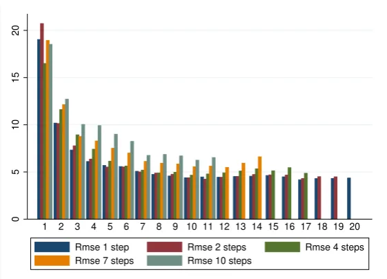
1 2 3 4 5 6 7 8 9 10 11 12 13 14 15 16 17 18 19 20 Rmse 1 step Rmse 2 steps Rmse 4 steps Rmse 7 steps Rmse 10 steps

Figure 6: Average RMSE across groups as a function of the period and for different forecasting horizons.

individual predictions in periodtfor the pricek-periods ahead:

RM SEt,k =

s P6

i=1(ipet,t+k−pf)2

6

From Figure 6, it is evident that short-run expectations do not converge to the fundamental value, although the RMSE reduces over time. The same pattern is observed for long-run ex-pectations. When comparing convergence for different time horizons from Figure 6, we observe that the RMSE increases marginally with the forecasting time horizon. As a first approximation, we can state that the degree of convergence of expectations is largely independent of the time horizon. It seems that the fundamental value is not the main determinant of the dynamics of short- and long-run expectations. Given our results, we can conclude then that the REE is not a good descriptor for subjects’ expectations as well as price dynamics.

3

Computational Learning Approach

3.1

Learning Algorithms

negligible effect on the price dynamics. So we can assume that long-run expectations dynamics reflect short-run expectation dynamics and the price evolution.

3.1.1 The Heuristic Switching Model

In the following, we list the four heuristics of the HSM as introduced in the original paper by Anufriev and Hommes [2012]. We briefly describe those rules adapting them to our notation. We label the four rules according to the index h= 1, ..,4, indicating the corresponding forecasting price ashpet,t. Note that the left sub-indexhdenotes now the heuristic instead of the subject.

The heuristics are:

• Adaptive rule (ADA): it is a weighted average of the last prediction and the last realized price.

1pe_t,t=αpt₋1+ (1−α)pe_t

−1,t−1 α= 0.65 (3)

• Weak trend following rule (WTR): according to this rule, agents take into account the last realization of the market price and adjust their prediction extrapolating the market trend. The coefficient of proportionality is smaller than one, so the “weakness” in the name of the rule.

2pet,t=pt−1+w(pt−1−pt−2) w= 0.4

• Strong trend following rule (STR): it is structurally identical to the WTR. The difference is given by the weight assigned to the extrapolative parameter, in this case higher than 1.

3pet,t=pt₋1+s(pt₋1−pt₋2) s= 1.3

• Learning and adjustment rule (LAA): the first part is thetime-dependent anchor given by the average of the last observed price and the mean of the past prices. The second term of the equation represents the extrapolative term. Note here the unitary coefficient of the extrapolative term.

4pet,t= 0.5(p av

t₋1+pt−1) + (pt−1−pt−2)

The learning mechanism is based on the relative profitability of each forecasting rule among the four fixed rules. Agents do not learn new rules and do not modify them neither. They rank the different rules and choose the one that better performed in the recent past. The switching mechanism is based on a performance measure Uh,t that depends on the quadratic forecasting

error. The performance measureUh,t is given by:

Uh,t₋1=−

pt₋1−hpet−1,t−1 2

+η Uh,t₋2, h= 1, ...,4

where the parameter 0≤η≤1 represents the “memory” of agents, meaning the weight assigned to past errors. We setη= 0.7, following Hommes [2013].

using the discrete choice model with asynchronous updating as in Diks and Van Der Weide [2005]. The updating equations are:

nh,t=δ nh,t−1+ (1−δ)

exp(β Uh,t−1)

Zt₋1

, (4)

Zt₋1= 4

X

h=1

exp(β Uh,t₋1), (5)

where 0 < δ ≤ 1 denotes the share of agents that update their choice; the parameter β ≥ 0 represents the intensity of choice and it determines the switching speed to the most successful rule. Zt₋1is a normalization factor. We considerδ= 0.9 and β= 0.4 as in Hommes [2013]. We

compute the expected price as a weighted average across the different expectations given by the four rules:

¯

pet,t=

4

X

h=1

nh,t₋1hpet,t.

and we insert this value in eq. (1) to compute the resulting market price.

The literature of LtFE has shown that the HSM can fairly well reproduce the properties of short-run expectations in different experimental settings. However, the HSM, at least in its present form, cannot be a suitable model to reproduce the observed proprieties of long-run expectations. Note, in fact, that three out of four rules (heuristics 2, 3 and 4) depend exclusively on past prices. As a consequence, when using those rules, all artificial agents will share exactly the same prediction for future prices. It means that the agents’ long-run predictions using those rules are constant values, independent of the forecasting horizon and the agent identity:

hpet,t+k=hpet,t h= 2,3,4

The variable hpet,t is a function of the past price, whose value depends on the particular

heuristic considered. The only rule that can generate heterogeneous predictions across agents is the first one (ADA), since it depends on the past individual short-run prediction. If we iterate this rule, we obtain:

ipet,t+k =ipte−1,t−1(1−α)

k₊

pt−1 (1−(1−α)

k+1

). (6)

where k denotes the forecasting horizon8_{. Note that we have replaced the index}

h = 1 with the identity of the agent i, since the k-steps-ahead prediction depends on the agent identity through the short-run expectation submitted in period t−1, i.e. ipet−1,t−1. Eq. (6) implies

that, independently of the subjects’ one-step-ahead prediction, long-run predictions exponentially converge to the last realized pricept₋1. Already for a forecasting horizon approximatively equal

to 3, we obtain essentiallyipet,t+k ≈pt₋1. Such behaviour is in contradiction with the observed

data. According to eq. (6), in fact, the heterogeneity of subjects’ long-run expectations vanishes, instead of increasing as in Figure 3. In its present form, therefore, the HSM cannot be used to describe in a meaningful way the subjects long-run predictions in our LtFE experiment, since it systematically underestimates the heterogeneity of subjects’ long-run expectations.

8

3.1.2 The Exploration-Exploitation Algorithm

Given the drawbacks of the HSM in reproducing long-run expectation properties, we propose the Exploration-Exploitation Algorithm to describe both, short and long-run expectations and the corresponding price dynamics. Within the EEA we do not impose a finite set of decision rules. Instead, agents choose their actions from a distribution of feasible actions whose main determinants, mean and variance, evolve adaptively based on past price dynamics. In particular agents’ learning is based on the ability to adapt the range of variation of their actions as they acquire more information when observing price dynamics.

In order to adapt the EEA to our experimental setting, we consider the subjects’ predictions for future prices at different time horizons to be theactions of artificial agents. Theexploration space is the considered range of prices divided in a discrete grid of 100 steps, so that each step corresponds to a feasible action. Each action will have a different probability to be chosen, depending on its past performance. Moreover, the exploration space adapts over time, i.e. the range of actions changes according to the realized price in the last period and to its past fluctu-ations. In particular, the range is centred in the last observed price (pt₋1) and the amplitude of

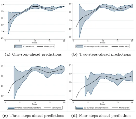
the range is proportional to the standard deviation of the past prices. In other words, the anchor is the last price and the adjustment is made according to the observed volatility of the time series of market prices. The mechanics of the algorithm is based on the experimental evidence suggesting that subjects coordinate their predictions anchoring them around the last observed price. The exploration space adapts to the new market conditions, typically reducing over time. As we have shown when describing the experimental results, the heterogeneity among indi-vidual predictions reduces rapidly in the first few periods. Within the framework of the EEA, we can interpret this dynamics as the fact that subjects tend to explore a large space in the first periods, when they possess few pieces of information to characterize the price dynamics, while they prefer to adopt the exploitation strategy afterwards, when the “cost of exploration” is relatively high.9 _{In order to better illustrate our interpretation of the EEA, we show in Figure 7}

an example of how the exploration space reduces over time. We compute the standard deviation of the subjects’ individual predictions from the experimental data each period for the price one, two, three and four steps-ahead. We observe that, in early periods, subjects count with a few pieces of information to have a precise idea about the price evolution and therefore the range of their short and long-run predictions is wider. After few periods of learning, subjects tend to play the exploitation strategy, i.e. to submit forecasts narrowly centred inpt−1. This is

partic-ularly true for the one-step-ahead predictions for which subjects receive an immediate feedback Colasante et al. [2016].

Let us formalize the mathematical description of the EEA algorithm. All agents have a set of n= 100 feasible actions denoted asAt ={a1t, a2t, ..., ant} where a1t < a2t < ... < ant, that

is common to all agents, where ajt denotes a single element inAt, being j ∈ {1, ...,100}. The

set At changes every period depending on the last market price and the standard deviation of

past prices. The range of the set is given by (pt₋1−5σp, pt₋1+ 5σp) whereσp is the standard

deviation of the last three market prices. Note thata1t=pt₋1−5 σp anda100t=pt₋1+ 5σp.

At the beginning of period t, agent iselects an action i˜at=ipet,tfrom At, that corresponds

to the agenti’s expected price at the end of periodt, i.e. the one-step-ahead prediction. Besides the one-step-ahead predictions, agent i chooses three more actions i˜akt =ipet,t+k from the

cor-responding set of actions Ak

t ={ak1t, ak2t, ..., aknt}, wherek∈ {1,2,3}. Each one of these actions

represents the agenti’s long-run expectations up to four-steps-ahead. Also the elements of those sets change every period. In particular, the range of Ak

t is centred on pt−1, as in the case of 9

45

50

55

60

65

70

0 5 10 15 20

Period

SD predictions Market price

(a)One-step-ahead predictions

50

55

60

65

70

0 5 10 15 20

Period

SD two steps-ahead predictions Market price

(b)Two-steps-ahead predictions

55

60

65

70

0 5 10 15 20

Period

SD trhee steps-ahead predictions Market price

(c)Three-steps-ahead predictions

55

60

65

70

75

0 5 10 15 20

Period

SD four steps-ahead predictions Market price

(d)Four-steps-ahead predictions

Figure 7: The continuous line represents the market price and the shadow area refers to one standard deviation of individual predictions. The data refers to Group 1.

short-run predictions, but, differently fromAt, its amplitude is constant over time and does not

depend on the price evolution. Since the long-run profit function used in the experimental design is a step function, we assume that the maximum range for the agents long-run predictions is 15.10

The range for the actions that belong toAkt is therefore (pt−1−15, pt−1+15).

11 _{As an illustrative}

example, Figure 8 shows in panel (a) how the range of set At (short-run predictions) reduces

over time, and in panel (b), how the range of setAkt (long-run predictions) remains constant over

time.

Once all agents choose their actions the market price is computed according to eq. (1). Agents then evaluate the performance of all feasible actions using a fitness function. We introduce two different measures: the first one to evaluate the actions in the setAt, that refers to the agents’

short-run predictions, denoted asVt; the second one to evaluate the actions in the setsAkt that

refer to the agents’ long-run predictions, denoted asVk

t. The main difference is that we consider

the quadratic distance between the agent’s action and the realized price to evaluate short-run predictions, while we consider the absolute distance to evaluate the subject’s long-run predictions. This difference is introduced in order to replicate the profit functions we use in the experiment. The value of the fitness measures are:

iVj,t=−(pt−iajt)2+φsiVj,t−1, (7) 10

Note that, following the payment schedule used to reward the subjects long-run expectations in the experi-ment, if the absolute difference between the price and the long-run prediction is higher than 15, the profit is equal to zero.

11

(a)Short-run predictions (At) (b)Long-run predictions (A4t)

Figure 8: Evolution of the range of the agents’ decision sets (one-step-ahead and four-steps-ahead predictions) for different periods.

iVkj,t=−|pt−iakjt|+φ k

iVkj,t₋1 (8)

The parameters φs_{and φ}k _{represent the weight assigned to the past forecasting errors. We set}

φs_{= 0.3 andφ}k _{= 0.5.}12

We then introduce a probability distribution associated to the setAtfor each agenti.

Essen-tially, all agents have the same set of actions, however the fitness measures and the associated probability distributions differ among agents depending on the individual past performance. Note the dependence in eqs. (7) and (8) of the measures on the individual agent’s identity. For the choice of short-run predictions, letipjt be the probability that agent i selects action iajt from

the set At, such that 0 ≤ipjt ≤1 and P

100

j=1ipjt = 1. The probability to select action iajt is

given by:

ipjt=

exp(γ·iVj,t)

P100

j=1exp(γ·iVj,t)

, (9)

whereγ∈[0,∞) represents the intensity of choice as in the HSM. We setγ= 0.2. For the choice concerning the long-run predictions we introduce analogue functions to compute the probabilities attached to each one of the actions referring to the long-run expectations:

ipkjt=

exp(γ·iVkj,t)

P100

j=1exp(γ·iV

k j,t)

(10)

According to the probability distributions in eqs. (9) and (10) in each period t each agent randomly chooses four actions i˜at and ia˜tk , wherek ∈ {1,2,3} (one short-run prediction and

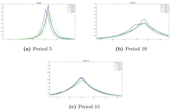
three long-run predictions). Figures 9 and 10 illustrate an example of the probability distributions associated to each action for the different agents and time horizon, specifically one and four-steps-ahead actions at different time periods of a simulation. We can clearly observe a certain degree of heterogeneity among agents and time horizons, which depends on the past history of the agents’ choices.

3.2

Simulation results

After a comprehensive description of the two algorithms, in this section we compare their per-formance in replicating the experimental results.

12

(a)Period 5 (b)Period 10

(c)Period 15

Figure 9: Examples of the probability distributions of one-step-ahead prediction for each agent for three different periods.

(a)Period 5 (b)Period 10

(c)Period 15

55

60

65

70

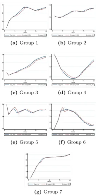
0 5 10 15 20 Period Exp_price Simulated_HSM Simulated_EE

(a)Group 1

55

60

65

0 5 10 15 20 var11 Exp_price Simulated_HSM Simulated_EE

(b)Group 2

60

65

70

75

0 5 10 15 20 Period Exp_price Simulated_HSM Simulated_EE

(c)Group 3

60

65

70

0 5 10 15 20 Period Exp_price Simulated_HSM Simulated_EE

(d)Group 4

55

60

65

0 5 10 15 20 Period Exp_price Simulated_HSM Simulated_EE

(e)Group 5

62

64

66

68

70

0 5 10 15 20 Period Exp_price Simulated_HSM Simulated_EE

(f )Group 6

45

50

55

60

65

0 5 10 15 20 Period Exp_price Simulated_HSM Simulated_EE

(g)Group 7

Figure 11: Simulation results based on the HSM and the EEA. The continuous black line is the exper-imental market price, the blue line is the market price generated using the HSM and the dashed grey line is the market price generated using the EEA.

3.2.1 Comparing the HSM and EEA to describe short-run expectations

We calibrate the HSM using the experimental market price in the first three periods. We need, in fact, three prices to compute the expectations in some of the heuristics. At the beginning of the simulation, we assign the same weight to each rule, i.e. nh,1 = 0.25,∀h. Starting from

period three we compute the fitness measure and weightnh,3 associated to each heuristic. For

the subsequent periods we iterate the algorithm detailed in the previous section.

We calibrate then the EEA using the experimental individual predictions and the first three realized prices, since the range of the action sets depend on the three past realized prices. To compute the market price using the EEA, in each period we make six (the number of subjects in the group) independent draws from the six different distributions of the short-run expectations. Once we have the individual predictions we use eq. (1) to compute the market price and iterate then the algorithm.

data are of the same order of magnitude. In particular, the EEA shows a better performance in half of the groups. So we can safely conclude that the EEA achieves similar results as the HSM in replicating the price dynamics.

Table 1: Mean Squared Error of the HSM and EEA in describing the time series of experimental market prices.

HSM EEA

Group 1 0.37 0.29

Group 2 0.06 0.06

Group 3 0.44 0.13

Group 4 0.33 0.13

Group 5 0.22 0.38 Group 6 0.19 0.16

Group 7 0.15 0.77

The next step is to check the performance of the two algorithms in replicating coordination and convergence of individual expectations. To analyse the coordination of expectations, we compute the standard deviation among the individual one-step-ahead predictions in each group of the EEA. In the case of HSM, the procedure is not straightforward since the HSM does not replicate the individual predictions, but instead the frequencies in the use of the heuristics across a large population of agents. So, we compute the standard deviation of the expectations considering the frequencies in the use of heuristics as given by eq. (4). Figure 12 shows the comparison of the two algorithms with respect to the experimental data. Note that the first three periods coincide with the experimental data because of the calibration procedure of the two algorithms. The qualitative behavior of the experimental data is well captured by the simulated results of the tow algorithms, without any systematic difference. Figure 13 shows a good agreement between simulated and experimental data.

Comparing the results of Table 1 to the performance of the HSM reported in other papers (Anufriev and Hommes [2012], Anufriev et al. [2013b] and Bao et al. [2012], we can see that the MSEs are of the same order of magnitude. Given that, filtering our experimental prices with the HSM, we obtain essentially similar aggregate results, we can state that eliciting long-run expectations does not affect the price dynamics with respect the baseline LtFE, i.e. when eliciting just one-step-ahead expectations. This conclusion allows us to discard the existence of a significant impact of inter-temporal hedging strategies followed by the subjects. Similar behavior has been reported by Hanaki et al. [2016] in an experimental setting with trading studied by Haruvy et al. [2007].

3.2.2 Long-run expectations in EEA

To the best of our knowledge, this is the first attempt in the literature on LtFEs to reproduce indi-vidual long-run expectations using a learning algorithm. Despite the fact that in the experiment we elicit the expectations for the whole time horizon, we replicate the individual expectations up to four steps-ahead. Our choice represents a good compromise between considering the whole time-span and having a sufficient statistics to analyse the properties of the experimental data as a function of the time horizon.

0

5

10

15

1 2 3 4 5 6 7 8 9 10 11 12 13 14 15 16 17 18 19 20 Sd experiment Sd HSM Sd EE

Figure 12: Coordination: average across groups of the standard deviation of one-step-ahead predictions per period. Blue bars refer to experimental data, red bars refer to HSM and green bars refer to EEA. The histograms of the simulated data are an average over 100 Monte Carlo iterations of the EEA and HSM.

0

5

10

1 2 3 4 5 6 7 8 9 10 11 12 13 14 15 16 17 18 19 20 RMSE Experiment RMSE HSM RMSE EE

-1

-.5

0

.5

1

Correlation 1 step (exp) Correlation 1 step (simu) Correlation 2 step (exp) Correlation 2 step (simu) Correlation 3 step (exp) Correlation 3 step (simu) Correlation 4 step (exp) Correlation 4 step (simu)

Figure 14: Box-plots of the correlation coefficients between the time series of prices and the individual subjects’ expectations at different time horizons compared to the corresponding values for the simulated data.

(iv) the convergence of long-run expectations to the fundamental value. Note that here we do not have an aggregate variable like the market price, but just individual long-run predictions. Furthermore, we cannot compare the performance of our algorithm to an alternative learning specification, since,as previously illustrated, the HSM, in its present form can not be implemented to model individual long-run expectations.

Figures 15, 16, 17 show the simulated individual long-run expectations confronted to the experimental data of three representative subjects belonging to groups 1, 4 and 5. Each line represents the predictions submitted by subjectiin period tfor the price at the end of the fol-lowing 2, 3 and 4 periods ahead. In other words, each series represents respectively: ipet,t+1(blue

line),ipet,t+2 (red line) andipet,t+3 (green line) ∀t. The EEA describes fairly well the individual

long-run predictions. However, the simulated time series of expectations exhibit a “rougher” path compared to the smooth time series observed in the experimental data, We conjecture that the experimental expectations possess a higher degree of time-correlations among the predictions at different time horizons than what results from the EEA. Consider that in the EEA, the three predictions (i˜a1t, ia˜2t andi˜a3t) are independent draws from the corresponding probability

distri-butions of actionsipjtk, that evolve independently without any explicit conditional dependence.

Our results speak in favour of the existence of a conditional dependence among the long-run expectations, that can be implemented in future modifications of the EEA or alternatively in a modified version of the HSM.

The EEA assumes that agents actions are anchored around the last realized price. The good performance of the algorithm leads us to infer that the last price turns out to be a strong anchor for long-run expectations (at least up to four period ahead) even if the feedback given by the profit comes with a delay. Figure 14 shows a stable correlation between the market price and the expectations at different time horizons. The EEA is structurally built on using the last price as an anchor. However, it is noticeable how the EEA captures extremely well the subjects’ heterogeneity in incorporating the last realized price in their expectations.

40

50

60

70

80

0 5 10 15 20

var11

2 STEPS Exp 3 STEPS Exp 4 STEPS Exp

(a)Experimental data

40

50

60

70

80

0 5 10 15 20

var11

2 STEPS Sim 3 STEPS Sim 4 STEPS Sim

(b)Simulated data

Figure 15: Illustrative example of a time series of long-run predictions of an individual subject in group 1 for different time horizons (2, 3 and 4 steps ahead) as compare to the simulated data.

20

40

60

80

100

0 5 10 15 20

Period

2 STEPS Exp 3 STEPS Exp 4 STEPS Exp

(a)Experimental data

20

40

60

80

100

0 5 10 15 20

Period

2 STEPS Sim 3 STEPS Sim 4 STEPS Sim

(b)Simulated data

Figure 16: Illustrative example of a time series of long-run predictions of an individual subject in group 4 for different time horizons (2, 3 and 4 steps ahead) as compared to the simulated data.

30

40

50

60

70

80

0 5 10 15 20

var11

2 STEPS Exp 3 STEPS Exp 4 STEPS Exp

(a)Experimental data

30

40

50

60

70

80

0 5 10 15 20

Period

2 STEPS Sim 3 STEPS Sim 4 STEPS Sim

(b)Simulated data

0

5

10

15

20

1 23 4 5 6 7 8 9 10 11 12 13 14 15 16 17 18 19 20 Sd 2steps experiment Sd 2steps Simulation

(a)Two-steps-ahead

0

5

10

15

12 3 4 5 6 7 8 9 10 11 12 13 14 15 16 17 18 19 20 Sd 3steps Experiment Sd 3steps Simulation

(b)Three-steps-ahead

0

5

10

15

20

12 3 4 5 6 7 8 9 10 11 12 13 14 15 16 17 18 19 20 Sd 4steps Experiment Sd 4steps Simulation

(c)Four-steps-ahead

Figure 18: Coordination of individual long-run expectations comparing simulated and experimental data. The histograms of the simulated data are an average over 100 Monte Carlo iterations of the EEA.

periods ahead. It shows that the degree of coordination resulting from the simulated data is fairly close to the degree of coordination of experimental data. Additionally, the EEA is able to reproduce the more persistent heterogeneity observed for the long-run predictions as compared to the degree of coordination of the one-step-ahead predictions.

In order to measure the performance of the EEA to reproduce the convergence of individual expectations to the fundamental value, in Figure 19, we compare the RMSE of simulated and experimental data. We are able to conclude that the EEA is able to replicate also the lack of convergence.

4

Conclusion

0

5

10

15

20

1 23 4 5 6 7 8 9 10 11 12 13 14 15 16 17 18 19 20 RMSE Experiment RMSE Simulation

(a)Two-steps-ahead

0

5

10

15

20

12 3 4 5 6 7 8 9 10 11 12 13 14 15 16 17 18 19 20 RMSE Experiment RMSE Simulation

(b)Three-steps-ahead

0

5

10

15

20

12 3 4 5 6 7 8 9 10 11 12 13 14 15 16 17 18 19 20 RMSE Experiment RMSE Simulation

(c)Four-steps-ahead

Figure 19: Convergence of individual long-run predictions to the fundamental value for different time horizons comparing simulated and experimental data. The histograms of the simulated data are an average over 100 Monte Carlo iterations of the EEA.

long-run expectations, due to a higher degree of uncertainty faced by a subject when predicting the future behavior of the others.

In the second part of the paper, we introduce an adaptive learning algorithm in order to reproduce individual short and long-run expectations: the Exploration-Exploitation Algorithm. Such algorithm incorporates the bounded rational behavior of subjects by assuming that their expectations are centred on the last observed price and their range varies according to the most recent price fluctuations. We can surely cast our algorithm into the well-known anchor and adjustment behavioral framework. In order to evaluate the goodness of fit of our algorithm, we compare it to the well-established Heuristic Switching Model proposed by Anufriev and Hommes [2012] to model short-run expectations and market price dynamics. The computational part of the paper shows that the two learning algorithms perform equally well in describing the short-run dynamics of the experimental data. Although structurally different, the two algorithms share the same basic behavioral principle: anchor and adjustment. The fact that both satisfactorily describe the experimental data signals that subjects follow a similar general heuristic principle. Additionally, the good performance of the EEA to reproduce the long-run expectations dynamics generalizes and reinforces such conclusion.

other information sources, such as aggregate information on subjects’ long-run expectations, public announcements of policy measures (monetary policies with or without targeted level of inflations) or future changes of the fundamentals.

Acknowledgement

The authors are grateful for funding the Universitat Jaume I under the project P11B2015-63 and the Spanish Ministry Science and Technology under the project ECO2015-68469-R.

Compliance with Ethical Standards

References

Mikhail Anufriev and Cars Hommes. Evolutionary selection of individual expectations and ag-gregate outcomes in asset pricing experiments.American Economic Journal: Microeconomics, 4(4):35–64, 2012.

Mikhail Anufriev, Cars Assenza, Tiziana and, and Domenico Massaro. Interest rate rules and macroeconomic stability under heterogeneous expectations.Macroeconomic Dynamics, 17(08): 1574–1604, 2013a.

Mikhail Anufriev, Cars H Hommes, and Raoul HS Philipse. Evolutionary selection of expectations in positive and negative feedback markets.Journal of Evolutionary Economics, 23(3):663–688, 2013b.

Masahiro Ashiya. Testing the rationality of japanese gdp forecasts: the sign of forecast revision matters. Journal of economic behavior & organization, 50(2):263–269, 2003.

Tiziana Assenza, Te Bao, Cars Hommes, and Domenico Massaro. Experiments on expectations in macroeconomics and finance. In Experiments in macroeconomics, pages 11–70. Emerald Group Publishing Limited, 2014.

Tiziana Assenzaa, Peter Heemeijerc, Cars Hommesb, and Domenico Massarob. Individual ex-pectations and aggregate macro behavior. Technical report, 2011.

Peter Auer, Nicolo Cesa-Bianchi, and Paul Fischer. Finite-time analysis of the multiarmed bandit problem. Machine learning, 47(2-3):235–256, 2002.

Te Bao and Li Ding. –nonrecourse mortgage and housing price boom, bust, and rebound. Real Estate Economics, 2015.

Te Bao, Cars Hommes, Joep Sonnemans, and Jan Tuinstra. Individual expectations, limited rationality and aggregate outcomes. Journal of Economic Dynamics and Control, 36(8):1101– 1120, 2012.

Te Bao, John Duffy, and Cars Hommes. Learning, forecasting and optimizing: An experimental study. European Economic Review, 61:186–204, 2013.

William A Brock and Cars H Hommes. Heterogeneous beliefs and routes to chaos in a simple asset pricing model. Journal of Economic dynamics and Control, 22(8-9):1235–1274, 1998.

Sean D Campbell and Steven A Sharpe. Anchoring bias in consensus forecasts and its effect on market prices. Journal of Financial and Quantitative Analysis, 44(02):369–390, 2009.

Benoit Cœur´e. Monetary policy in the crisis – confronting short-run challenges while anchoring long-run expectations. Technical report, Speech by Benoit Cœur´e, Member of the Executive Board of the ECB at the Journ´ees de l’ AFSE 2013, 2013.

Annarita Colasante, Simone Alfarano, Eva Camacho-Cuena, Mauro Gallegati, et al. Long-run expectations in a learning-to-forecast experiment. Technical report, 2016.

Camille Cornand et al. Does inflation targeting matter? an experimental investigation. An Experimental Investigation (October 17, 2013), 2013.

Ippei Fujiwara, Hibiki Ichiue, Yoshiyuki Nakazono, and Yosuke Shigemi. Financial markets forecasts revisited: Are they rational, stubborn or jumpy? Economics Letters, 118(3):526– 530, 2013.

Gabriele Galati, Peter Heemeijer, and Richhild Moessner. How do inflation expectations form? new insights from a high-frequency survey. 2011.

Refet S Gurkaynak, Brian Sack, and Eric Swanson. The sensitivity of long-term interest rates to economic news: evidence and implications for macroeconomic models. The American Eco-nomic Review, 95(1):425–436, 2005.

Nobuyuki Hanaki, Eizo Akiyama, and Ryuichiro Ishikawa. A methodological note on eliciting price forecasts in asset market experiments. 2016.

Ernan Haruvy, Yaron Lahav, and Charles Noussair. Traders’ expectations in asset markets: experimental evidence. The American Economic Review, 97(5):1901–1920, 2007.

Peter Heemeijer, Cars Hommes, Joep Sonnemans, and Jan Tuinstra. Price stability and volatility in markets with positive and negative expectations feedback: An experimental investigation.

Journal of Economic dynamics and control, 33(5):1052–1072, 2009.

Cars Hommes. Behavioral rationality and heterogeneous expectations in complex economic sys-tems. Cambridge University Press, 2013.

Cars Hommes and Thomas Lux. Individual expectations and aggregate behavior in learning-to-forecast experiments. Macroeconomic Dynamics, 17(02):373–401, 2013.

Cars Hommes, Joep Sonnemans, Jan Tuinstra, and Henk van de Velden. A strategy experiment in dynamic asset pricing. Journal of Economic Dynamics and Control, 29(4):823–843, 2005.

Carsien Harm Hommes. Financial markets as nonlinear adaptive evolutionary systems. 2001.

Dimitris E Koulouriotis and A Xanthopoulos. Reinforcement learning and evolutionary algo-rithms for non-stationary multi-armed bandit problems. Applied Mathematics and Computa-tion, 196(2):913–922, 2008.

Robert E Lucas Jr. Asset prices in an exchange economy. Econometrica: Journal of the Econo-metric Society, pages 1429–1445, 1978.

Charles F Manski. Measuring expectations. Econometrica, 72(5):1329–1376, 2004.

Ramon Marimon, Stephen E Spear, and Shyam Sunder. Expectationally driven market volatility: an experimental study. Journal of Economic Theory, 61(1):74–103, 1993.

Yoshiyuki Nakazono. Heterogeneity and anchoring in financial markets. Applied Financial Eco-nomics, 22(21):1821–1826, 2012.

Amos Tversky and Daniel Kahneman. Judgment under uncertainty: Heuristics and biases.

science, 185(4157):1124–1131, 1974.

A

Screenshot and Instructions

20

40

60

80

0 5 10 15 20 Period

(a)Period 1

20

40

60

80

0 5 10 15 20

Period

(b)Period 2

40

50

60

70

80

0 5 10 15 20 Period

(c)Period 3

55 60 65 70 75 80

0 5 10 15 20 Period

(d)Period 4

50

60

70

80

90

0 5 10 15 20

Period

(e)Period 5

0

50

100

0 5 10 15 20 Period

(f ) Period 6

0

50

100

0 5 10 15 20 Period

(g)Period 7

0

50

100

0 5 10 15 20

Period

(h)Period 8

0

50

100

0 5 10 15 20 Period

(i) Period 9

50

60

70

80

90

0 5 10 15 20 Period

(j)Period 10

0

50

100

0 5 10 15 20

Period

(k)Period 11

0

50

100

0 5 10 15 20 Period

(l) Period 12

0

50

100

0 5 10 15 20 Period

(m)Period 13

0

50

100

0 5 10 15 20

Period

(n)Period 14

0

50

100

0 5 10 15 20 Period

(o)Period 15

0

50

100

0 5 10 15 20 Period

(p)Period 16

0

50

100

0 5 10 15 20

Period

(q)Period 17

0

50

100

0 5 10 15 20 Period

20

40

60

80

100

0 5 10 15 20 Period

(a)Period 1

40 50 60 70 80 90

0 5 10 15 20

Period

(b)Period 2

50

60

70

80

90

0 5 10 15 20 Period

(c)Period 3

55

60

65

70

75

0 5 10 15 20 Period

(d)Period 4

0

50

100

0 5 10 15 20

Period

(e)Period 5

0

50

100

0 5 10 15 20 Period

(f ) Period 6

0

50

100

0 5 10 15 20 Period

(g)Period 7

0

50

100

0 5 10 15 20

Period

(h)Period 8

0

50

100

0 5 10 15 20 Period

(i) Period 9

0

50

100

0 5 10 15 20 Period

(j)Period 10

0

50

100

0 5 10 15 20

Period

(k)Period 11

0

50

100

0 5 10 15 20 Period

(l) Period 12

0

50

100

0 5 10 15 20 Period

(m)Period 13

0

50

100

0 5 10 15 20

Period

(n)Period 14

0

50

100

0 5 10 15 20 Period

(o)Period 15

0

50

100

0 5 10 15 20 Period

(p)Period 16

0

50

100

0 5 10 15 20

Period

(q)Period 17

0

50

100

0 5 10 15 20 Period

(r) Period 18

20

40

60

80

100

0 5 10 15 20 Period

(a)Period 1

30 40 50 60 70 80

0 5 10 15 20

Period

(b)Period 2

45 50 55 60 65 70

0 5 10 15 20 Period

(c)Period 3

0

50

100

0 5 10 15 20 Period

(d)Period 4

0

50

100

0 5 10 15 20

Period

(e)Period 5

0

50

100

0 5 10 15 20 Period

(f ) Period 6

0

50

100

0 5 10 15 20 Period

(g)Period 7

0

50

100

0 5 10 15 20

Period

(h)Period 8

0

50

100

0 5 10 15 20 Period

(i) Period 9

0

50

100

0 5 10 15 20 Period

(j)Period 10

0

50

100

0 5 10 15 20

Period

(k)Period 11

0

50

100

0 5 10 15 20 Period

(l) Period 12

0

50

100

0 5 10 15 20 Period

(m)Period 13

0

50

100

0 5 10 15 20

Period

(n)Period 14

0

50

100

0 5 10 15 20 Period

(o)Period 15

0

50

100

0 5 10 15 20 Period

(p)Period 16

0

50

100

0 5 10 15 20

Period

(q)Period 17

0

50

100

0 5 10 15 20 Period

0 20 40 60 80 100

0 5 10 15 20 Period

(a)Period 1

50 60 70 80 90 100

0 5 10 15 20

Period

(b)Period 2

0 20 40 60 80 100

0 5 10 15 20 Period

(c)Period 3

30

40

50

60

70

0 5 10 15 20 Period

(d)Period 4

0 20 40 60 80 100

0 5 10 15 20

Period

(e)Period 5

30

40

50

60

70

0 5 10 15 20 Period

(f ) Period 6

0

50

100

0 5 10 15 20 Period

(g)Period 7

0

50

100

0 5 10 15 20

Period

(h)Period 8

40

50

60

70

0 5 10 15 20 Period

(i) Period 9

0 20 40 60 80 100

0 5 10 15 20 Period

(j)Period 10

0

50

100

0 5 10 15 20

Period

(k)Period 11

0

50

100

0 5 10 15 20 Period

(l) Period 12

0

50

100

0 5 10 15 20 Period

(m)Period 13

0

50

100

0 5 10 15 20

Period

(n)Period 14

0 20 40 60 80 100

0 5 10 15 20 Period

(o)Period 15

0

50

100

0 5 10 15 20 Period

(p)Period 16

0

50

100

0 5 10 15 20

Period

(q)Period 17

0

50

100

0 5 10 15 20 Period

(r) Period 18

20

40

60

80

100

0 5 10 15 20 Period

(a)Period 1

20

40

60

80

100

0 5 10 15 20

Period

(b)Period 2

40

60

80

0 5 10 15 20 Period

(c)Period 3

30 40 50 60 70 80

0 5 10 15 20 Period

(d)Period 4

40

50

60

70

80

0 5 10 15 20

Period

(e)Period 5

40

50

60

70

80

0 5 10 15 20 Period

(f ) Period 6

40 50 60 70 80 90

0 5 10 15 20 Period

(g)Period 7

40

50

60

70

80

0 5 10 15 20

Period

(h)Period 8

0

50

100

0 5 10 15 20 Period

(i) Period 9

0

50

100

0 5 10 15 20 Period

(j)Period 10

0

50

100

0 5 10 15 20

Period

(k)Period 11

0

50

100

0 5 10 15 20 Period

(l) Period 12

0

50

100

0 5 10 15 20 Period

(m)Period 13

0

50

100

0 5 10 15 20

Period

(n)Period 14

0

50

100

0 5 10 15 20 Period

(o)Period 15

0

50

100

0 5 10 15 20 Period

(p)Period 16

0

50

100

0 5 10 15 20

Period

(q)Period 17

0

50

100

0 5 10 15 20 Period

0 20 40 60 80 100

0 5 10 15 20 Period

(a)Period 1

0 20 40 60 80 100

0 5 10 15 20

Period

(b)Period 2

50

60

70

80

90

0 5 10 15 20 Period

(c)Period 3

60

70

80

90

0 5 10 15 20 Period

(d)Period 4

60

70

80

90

0 5 10 15 20

Period

(e)Period 5

60

70

80

90

100

0 5 10 15 20 Period

(f ) Period 6

0

50

100

0 5 10 15 20 Period

(g)Period 7

0

50

100

0 5 10 15 20

Period

(h)Period 8

0

50

100

0 5 10 15 20 Period

(i) Period 9

0

50

100

0 5 10 15 20 Period

(j)Period 10

0

50

100

0 5 10 15 20

Period

(k)Period 11

0

50

100

0 5 10 15 20 Period

(l) Period 12

0

50

100

0 5 10 15 20 Period

(m)Period 13

0

50

100

0 5 10 15 20

Period

(n)Period 14

0

50

100

0 5 10 15 20 Period

(o)Period 15

0

50

100

0 5 10 15 20 Period

(p)Period 16

0

50

100

0 5 10 15 20

Period

(q)Period 17

0

50

100

0 5 10 15 20 Period

(r) Period 18

0 20 40 60 80 100

0 5 10 15 20 Period

(a)Period 1

40

50

60

70

80

0 5 10 15 20

Period

(b)Period 2

40

60

80

100

0 5 10 15 20 Period

(c)Period 3

40

60

80

100

0 5 10 15 20 Period

(d)Period 4

40

60

80

100

0 5 10 15 20

Period

(e)Period 5

0

50

100

0 5 10 15 20 Period

(f ) Period 6

0

50

100

0 5 10 15 20 Period

(g)Period 7

0

50

100

0 5 10 15 20

Period

(h)Period 8

0

50

100

0 5 10 15 20 Period

(i) Period 9

0

50

100

0 5 10 15 20 Period

(j)Period 10

0

50

100

0 5 10 15 20

Period

(k)Period 11

0

50

100

0 5 10 15 20 Period

(l) Period 12

0

50

100

0 5 10 15 20 Period

(m)Period 13

0

50

100

0 5 10 15 20

Period

(n)Period 14

0

50

100

0 5 10 15 20 Period

(o)Period 15

0

50

100

0 5 10 15 20 Period

(p)Period 16

0

50

100

0 5 10 15 20

Period

(q)Period 17

0

50

100

0 5 10 15 20 Period