Munich Personal RePEc Archive
A contribution to the Quantity Theory of
Disaggregated Credit
Clavero, Borja
7 February 2017
Online at
https://mpra.ub.uni-muenchen.de/76657/
1
A Contribution to the Quantity Theory of Disaggregated Credit
Borja Clavero1
Last update: March 26, 20172
Abstract
In my view, Richard Werner is sitting on a pot of gold. In Werner (2014), he has shown the tremendous potential his ‘Quantity Theory of Credit’ has to reorient public policy and stimulate nominal GDP. Yet, his ideas do not seem to take root. In this paper my aim is to refine his theory and provide some improvements by constructing new empirical proxies of ‘bank credit for GDP transactions’—a quite arduous and open-ended task. I conclude that the theory is very promising, but it is still in a stage of maturation.
JEL: E50, G21.
Keywords: bank credit, Quantity Theory of Credit, credit-growth nexus, banking and the economy, disaggregation of credit, credit creation, flow of funds, national accounts.
Introduction
My aim in this paper is to make some improvements to Richard Werner’s Quantity Theory of Credit
(QTC). This theory was formulated in a series of papers in the 1990s in the context of the Japanese economy (cf. Werner, 1992, 1997) and was subsequently applied to Spain (cf. Werner, 2014), the UK (cf. Ryan-Collins, Werner and Castle, 2016; Lyonnet and Werner, 2012), and the Czech Republic (Bezemer and Werner, 2009), and Japan later again (cf. Werner, 2005, 2012; Voutsinas and Werner, 2011b). In its briefest formulation, the theory asserts the existence of a causal, robust, stable, autonomous relationship or mechanism3, relating two and only two variables: nominal GDP growth, and the growth rate of ‘bank credit used for GDP transactions’.
CRb = ‘bank credit for GDP transactions’ (see Table 1)
nGDP = ‘nominal GDP’
Causality running from CRb to nGDP. Let us refer to this stable and autonomous relation by:
ΔCRb
CRb →
ΔnGDP nGDP
1 Borja Clavero, M.Eng., M.Econ. Contact: [email protected]. 2 I certify that I have the right to deposit the contribution with MPRA
3 The following quote might clarify why I use the strange word mechanism: ‘ … the task of causal discovery is an induction game that
2
The mysterious variable CRb needs some clarification. Table 1 shows a two-by-two matrix disaggregating credit into four types, according to creditor type (rows) and the types of uses given to the credit instrument by the debtor (columns). Creditor types are classified as banks (more precisely, monetary financial institutions, MFIs) and banks (MFIs), each extending bank credit and non-bank credit, respectively. Credit instruments consist of loans and debt securities4 (Eurostat, 2013, p.
136). Loans are created when creditors extend funds to debtors, their value being measured in nominal terms. Debt securities are negotiable financial instruments serving as evidence of debt, measured in market value (Eurostat, 2013, p. 139). Importantly, equities and shares are not considered as credit instruments. These conceptual classifications follow the latest standard in national accounting, the
European System of Accounts 2010 (Eurostat, 2013). A more thorough presentation of the institutional sectors and financial instruments implied in Table 1 will be given in Section 3.
Uses of credit
GDP transactions Non-GDP transactions
Creditor Bank CR
b C
F b
Non-bank CRnb CFnb
Table 1. Disaggregation of credit by type of creditor and type of use
The upper left cell shows ‘bank credit used for GDP transactions’. This category refers to loans extended by banks, or debt securities purchased by banks from debtors, who devote the newly acquired funds in the form of bank deposits—which represent an asset to the debtor and a liability to the bank—to finance expenditures such as inventories in the case of private non-financial corporations, consumption in the case of consumers, and public services provision in the case of the public sector. The upper right cell contains credit issued by banks which is used to finance expenditures that are not part of GDP, such as the acquisiton of new land by the real estate sector, the acquisition of financial assets by hedge funds, or the financing of mergers and acquisitions by private non-financial corporations. The lower tier cells represent credit extended by the non-MFI sector, which is comprised of households, non-financial corporations, financial corporations except MFIs, insurance corporations, pension funds, general government, and non-profit institutions serving households. Wheras MFIs extend credit in the form of loans (bank-based finance), non-MFIs often lend to each other by purchasing commercial paper, corporate bonds, etc., from each other (capital market issuance). Equally, this non-MFI credit can be used to finance GDP and non-GDP transactions. This taxonomy of credit instruments by issuer and use will be used throughout the rest of the analysis.
Let me go back to the putative mechanism. If such a link exists, any other relationship between candidate explanatory variables and nominal GDP must be spurious or indirect. Supporting evidence for such claims has been collected, and thusfar it seems promising (cf. Werner, 1995, 1997, 1998, 1999, 2000, 2012a, 2012b, 2014; Ryan-Collins, Werner and Castle, 2016; Lyonnet and Werner, 2012; Werner, 2014; Bezemer and Werner, 2009). Yet, the state of this theory is still preliminary, that is, not entirely conclusive. This literature will be reviewed below.
But it is not so much its ‘inconclusiveness’ that impedes it from gaining widespread dissemination and acceptance. For one, all theories are in some sense incomplete, and second, scientists are paid to
3
come up with innovative ideas and to spot, appropriate and exploit ideas that might have the seeds of scientific utility in them. While some might simply think the theory is unripe fruit, and do not see anything in it for them, the core reasons of why the theory does not persuade economists lie elsewhere.
I can think of the following five factors that might explain the phenomenon:
1. Empirical search for good proxies is hard. The first factor is the lack of a ‘methodological benchmark’ providing clear guidance as to how good empirical proxies of CRb should be constructed. As I will explain, unlike traditional monetary aggregates, the variable ‘bank credit for GDP transactions’ is quite difficult to estimate correctly, and requires a meticulous disentangling of empirical bits and pieces. Several proxies have been crafted so far, but the authors do not give a thorough argumentation as to why the proxy was constructed in that
particular way. Many questions have been left unaddressed, and many choices seem arbitrary and not properly justified. This does a poor favour to the credence of the theory. For example, Werner constructed his original proxy of ‘bank credit for GDP transactions’ as the sum of loans to the private sector excluding ‘loans to the real estate sector, construction firms and non-bank financial institutions’ (Werner, 1997). But, as I will explain in more detail later, there are some arbitrary choices in there. Why not include loans to the government or households as well? Do not they contribute to GDP? Why not include other types of bank lending, such as governments borrowing from banks by issuing debt securities? Werner does not offer a justification; nor do the other authors, apart from mild allusions. If the theory is to realise its potential, a thorough exploration of the details in the proxy construction process is needed.
2. Irrefutability of QTC. The second factor, which is not on the surface but may have been perceived by some, is the fact that it is never possible to know for sure whether the proxy one has constructed is the ‘correct proxy’, and a process of ‘triangulation’ is required, that is, the combination of theoretically-informed search with empirical refinement. Thus, the theory can only be granted shades of plausibility, which renders it irrefutable in the strictest sense of the word. Refutability, falsifiability, or testability are core criteria that demarcates scientific from non-scientific theories5 (Popper, 1998, p. 40). Perhaps this makes QTC less attractive as a scientific endeavour.
3. Banks create money ex nihilo. Thirdly, the theory rests on a critically important premise about modern banking: banks create money (i.e., deposits) when they lend; banks do not intermediate funds from savers to borrowers, they create money, credit, and purchasing power ex nihilo by the act of lending to non-banks (Jakab and Kumhof, 2014, 2015; Benes, Kumhof and Laxton, 2014; Kumhof and Jakab, 2016; Berry et al., 2007; Bridges, Rossiter and Thomas, 2011; McLeay, Radia and Thomas, 2014; King, 2012; Tucker, 2007; Bundesbank, 2009, 2012; Borio and Disyatat, 2011; Turner, 2011, 2015a). This is a fact (see Section 1). But it is also a massive, widely misunderstood issue. Most textbooks teach the ‘loanable funds’, ‘intermediary’ conception of banks, and this is the view most economists hold. It is no wonder then that a theory that has this fact about money creation as its starting point eludes economists’ attention. 4. Stable an unstable velocities. A fourth factor that comes to mind is—not the premise of the theory—but its corollary. The theory asserts the existence of stable, robust relationship between
5 Pruzan (2016, p. 33) summarises Poppers conclusions on the properties of a scientific theory: (1) It is easy to obtain confirmations/
4
nominal GDP (a flow, measured in £/year) and ‘bank credit for GDP transactions’ (a stock, measured in £), the link between which is given by a variable usually referred to as ‘velocity’ (measured in years 1). A stable relationship between nGDP and C
R
b implies a constant velocity, as I will explain later. Seasoned monetary economists run away scared when told about stable velocities, and the 1980s trauma with the ‘equation that came apart at the seams’ (Goodhart, 1989) still resonates in their memory. It is thus natural that a theory like QTC finds no friends among them, who ultimately are its intended audience.
5. Theory-driven economics. The fifth factor is the predominance in economics of the theory-driven methodology as opposed to data-theory-driven. As I will show, constructing proxies of CRb requires an ardous search in the empirical data, across many types of financial instruments, assets, liabilities, balance sheets, flow-of-funds, national accounts, and so on. It is not controversial to say that economists generally do not feel comfortable with accouting.
As can be appreciated, it is not so much the weaknesses of the theory (the first two points) that hold it back, but also the idiosyncrasies of economics as a field (the last three points). These five factors have conspired against more broad dissemination and acceptance of QTC; perhaps there are more reasons, but these at least capture the core. It would do a good favour to the theory to try to reconcile a somewhat obscure theory and a skeptic, reluctant or even stubborn audience.
This is precisely the task I undertake in this paper. My aim is to give more credence to QTC by exploring its foundations, the literature, the theoretical predictions, and the empirical evidence supporting it. While I can do nothing about the fifth point, all the other points are touched upon in the paper.
This paper is structured as follows. In Section 1 (‘the elusive realities of banking and money creation’), I explore the details of money creation and identify and hopefully abate some of the misunderstandings on this topic. In Section 2 (‘the creditor-use decomposition of credit and links with nominal GDP’), I delve into the literature on the ‘credit-growth’ nexus and into the details of Werner’s findings and reasoning. In Section 3 (‘the process of constructing good empirical proxies of CRb’), I explore in great detail the concepts and steps involved in searching for empirical data in the proxy construction phase, starting from scratch until the final proxy is crafted. I also explore what choices and compromises emerge along the way, the points of uncertainty and vulnerability, and what can be done about them. Section 4 concludes.
A methodological note. I perform the study for the case of the UK economy, for three reasons. First, it has very good data sources, such as the Bank of England’s Bankstats, the Office for National Statistics, and the Debt Management Office. Second, studies on bank credit analogue to this one have already been performed by several authors (cf. Ryan-Collins, Werner and Castle, 2016; Lyonnet and Werner, 2012). Third, in Clavero (forthcoming), I use UK data to extend the ideas in this paper and in Werner (2014) to describe a new policy tool. The UK is a ‘liberal market economy’, which has been observed to typically display substantial fiscal and monetary policy discretion (Soskice, 2008). Would such a tool be implemented in Europe, it would likely be implemented in the UK first.
1.
The elusive realities of banking and money creation
‘In the real world, banks extend credit, creating deposits in the process, and look for the reserves later.’
5
The financial crisis has brought to the public’s attention a fact that has generated much perplexity and disbelief, namely, that leading economic theories and models, as well as influential advanced textbooks in macroeconomics and monetary economics, did not feature money (e.g. Woodford, 2003), or banks (Walsh, 2003; Woodford, 2003). Current cutting-edge macroeconomic models since the 1980s do not include credit, debt, or a financial sector (King 2012; Sbordone et al. 2010), nor are there borrowing constraints or risks of default in them (Goodhart and Hofmann, 2008). The dominant New Keynesian model of monetary economics ‘lacks an account of financial intermediation, so that money, credit and banking play no meaningful role’ (King, 2012), and ‘treat[s] intermediaries largely as a veil’ (Gertler and Kiyotaki, 2010). Similarly, in consumption theory, debt plays no causal role in determining the amount of spending6 (Bunn and Rostrom, 2014). DSGE models, considered state-of-the-art and widely
used among central bankers, do not include a financial sector, a deficiency not easily remedied due to their particular methodology and assumptions (Werner, 2012). As Olivier Blanchard put it with some regret, ‘we assumed we could ignore the details of the financial system’7.
The reason for not treating banks in macroeconomic models as analytically distinct actors is explained by the capacities attributed to them by theory. Banks, according to the dominant view, are functionally no different from other non-bank financial institutions: they gather deposits and lend these out (Werner, 2015). This view has come to be known as the ‘loanable funds’ or ‘financial intermediation’ model of banking. Deviants from that view have either been ignored or mocked (e.g., Krugman, 2012).
Though dominant today, this conception of banking enjoyed much less recognition during most part of the 20th century, during which it co-existed and alternated in predominance with at least two competitors (Werner, 2015).The oldest, the ‘credit creation theory’ of banking, maintains that each bank can individually create money ‘out of nothing’ through accounting operations, and does so when extending a loan. The ‘fractional reserve theory’ states that only the banking system as a whole can collectively create money, while each individual bank is a mere financial intermediary, gathering deposits and lending these out. The ‘financial intermediation theory’ considers banks as financial intermediaries both individually and collectively, rendering them indistinguishable from other non-bank financial institutions in their behaviour, especially concerning the deposit and lending businesses, being unable to create money individually or collectively8.
From the 1930s until the 1960s, the accepted view was the ‘credit creation theory’. The ‘deposit multiplier’ view was widely accepted in academic and policymaking circles between the 1930s and the late 1960s, and overlapped with the periods during which the ‘credit creation’ and ‘intermediary’ views dominated (Jakab and Kumhof, 2015). But since the 1960s, the position of the ‘credit creation’ view has weakened and the ‘financial intermediation’ perspective has replaced it eversince (Jakab and Kumhof, 2016).
Still, science is not monolithic, and some central bankers and policymaking authorities today give full endorsement to the ‘credit creation’ theory. The following quotes are a sample of the contemporary views of prominent economists working in different institutions:
‘… the banking system as a whole does not collect additional deposits from non-bank depositors, it creates additional deposits for non-bank borrowers. There are no pre-existing loanable funds, new funds materialize on the banker’s keyboard at the moment he makes a new loan.’
Jakab and Kumhof (2014), International Monetary Fund
6In the Modigliani and Brumberg (1979) model, consumption depends only on expected lifetime income and wealth, with households
smoothing spending over their lifetimes. Typically, households should borrow to help finance their consumption when they are young and their incomes are relatively low. They then repay that debt later in life as their incomes rise and they build up savings ahead of retirement, when income falls back again (Bunn and Rostrom, 2014)
7 Comments at IMF press conference, October 2012
6 ‘… bank loans give borrowers new purchasing power that did not previously exist’
Benes, Kumhof and Laxton (2014), International Monetary Fund ‘… in the real world, the key function of banks is the provision of financing, or the creation of new monetary purchasing power through loans’
Jakab and Kumhof (2015), International Monetary Fund ‘New funds are produced only with new bank loans (or when banks purchase additional financial or real assets), through book entries made by keystrokes on the banker’s keyboard at the time of disbursement. This means that the funds do not exist before the loan’
Kumhof and Jakab (2016), International Monetary Fund ‘… by far the largest role in creating broad money is played by the banking sector … when banks make loans they create additional deposits for those that have borrowed the money … Under the present system banks do not have to wait for depositors to appear and make funds available before they can on-lend, or intermediate, those funds. Rather, they create their own funds, deposits, in the act of lending.’
Berry et al. (2007), Bank of England ‘… the extension of loans mechanically creates deposits … Any transaction between the banking sector and the non-bank private sector will involve the creation or destruction of banking sector deposits and will thus affect the supply of broad money’
Bridges, Rossiter and Thomas (2011), Bank of England ‘When banks make loans they create additional deposits for those that have borrowed … Banks making loans and consumers repaying them are the most significant ways in which bank deposits are created and destroyed in the modern economy … Just as taking out a new loan creates money, the repayment of bank loans destroys money … in the modern economy, those bank deposits are mostly created by commercial banks themselves’
McLeay, Radia and Thomas (2014), Bank of England ‘When banks extend loans to their customers, they create money by crediting their customers’ accounts.’ Mervyn King (2012), former Governor of the Bank of England
‘The Bank [of England] supplies base money on demand at its prevailing interest rate, and broad money is created by the banking system’
Mervyn King (1994, p. 264), former Governor of the Bank of England, then Chief Economist and Executive Director of the Bank
‘Banks extend credit by simply increasing the borrowing customer’s current account … That is, banks extend credit [i.e. make loans] by creating money’
Paul Tucker (2007), Deputy Governor for Financial Stability, Bank of England (2009-2013)
‘The initial process of lending involves only the extension of an individual commercial bank’s balance sheet, an increase in assets from the freshly created loan and a matching increase in liabilities from the accompanying deposit created for the recipient of the loan.’
Rule (2015), Bank of England ‘The commercial banks can also create money themselves… in the eurosystem, money is primarily created by the extension of credit…’
7 account. ... The creation of deposit money is therefore an accounting transaction.’
Bundesbank (2012) ‘banks … create additional purchasing power in the form of deposits through the act of extending credit … Through the creation of deposits associated with credit expansion, banks can grant nominal purchasing power without reducing it for other agents in the economy … The banking system can … expand total nominal purchasing power’
Borio and Disyatat (2011), Bank of International Settlements ‘… the banking system does not simply transfer real resources, more or less efficiently, from one sector to another; it generates (nominal) purchasing power … Deposits are not endowment that precede loan formation; it is loans that create deposits’
Borio (2012), Bank of International Settlements ‘The banking system can thus create credit and create spending power – a reality not well captured by many apparently common sense descriptions of the functions which banks perform. Banks it is often said take deposits from savers (for instance households) and lend it to borrowers (for instance businesses) … But in fact they don’t just allocate preexisting savings, collectively they create both credit and the deposit money which appears to finance that credit.’
Adair Turner (2011), then Chairman of the Financial Services Authority ‘… banks do not just intermediate flows of already existing money from savers to borrowers, but create credit, money and purchasing power ex nihilo’
Adair Turner (2015a), former Chairman of the Financial Services Authority ‘When a bank extends a loan, it creates a deposit account, increasing the supply of money. … the creation of money and the creation of credit occur together’
Stiglitz and Greenwald (2003, p. 295), Columbia University and Columbia Business School ‘Banks lend to borrowers and create credit and money simultaneously … assets and liabilities of the bank have thus expanded simultaneously, and the bank has in essence created its own funding through the very process of lending … Because the new entries on both sides of the bank’s balance sheet are in the name of [the same person], there is no intermediation of loanable funds between savers and borrowers at the time the loan was made’
Markus K. Brunnermeier (Princeton), Harold James (Princeton), and Jean-Pierre Landau (SciencePo Paris) (2016, p. 160)
These voices convey the same message without a trace of ambivalence: commercial banks create deposits ex nihilo when they extend loans. Banks do not collect deposits so the can lend them out. In fact, bank deposits are simply a record of how much the bank itself owes its customers. So they are a liability of the bank, not an asset that could be lent out (McLeay, Radia and Thomas, 2014). Deposits, in turn, consitute the vast majority of ‘broad money’, with notes and coins—issued by central banks— constituting just 3%.
8
empirically examined (Werner, 2015).
The first empirical test published in a leading journal on this issue was Werner (2014), in which the author obtained the cooperation of Raiffeisenbank Wildenberg e.G., a cooperative bank in Lower Bavaria, to examine the actual operations and accounting entries taking place when a ‘live’ bank loan is granted and paid out. It was found that only the credit creation theory was consistent with the observed empirical evidence. The author states: ‘thus it can now be said with confidence for the first time— possibly in the 5000 years’ history of banking—it has been empirically demonstrated that each individual bank creates credit and money out of nothing’. In Werner (2015), the author performed a similar test, reaching the same conclusions.
The ‘money creation’ powers of banks can also be traced to the legal sphere. Werner (2014b) has shown that, in the UK context, what distinguishes banks from non-banks, and therefore allows them to do this, is that they are exempt from legal rules known as Client Money Rules, which are outlined in Chapter 7 (‘Client Money Rules’) of the Financial Conduct Authority Handbook 2016 (FCA, 2016). These rules require non-banks to hold retail client monies in trust, or off-balance sheet9. Banks, on the other hand, are allowed to keep retail customer deposits on their own balance sheet10. Depositors who deposit their money with a bank are therefore no longer the legal owners of this money, with the bank holding it in trust for them, but rather they are one of the general creditors of the bank. This implies that when non-banks disburse a loan to their clients, they need to give up either cash or their own bank deposits, while when banks disburse a loan, they do so by reclassifying an “accounts payable” liability (their obligation to disburse the loan in return for having received the right to receive future payments of principal and interest) as a “customer deposit” (Kumhof and Jakab, 2016). Outside the UK, the regulation of money creation differs in terminology, but on broad brush it is highly similar. Table 2 is taken from Burgess and Janssen (2007), and provides the details of which institutional units are able to create what types of instruments considered as ‘money’.
Country Money creators Instruments included
United Kingdom (M4) Banks and building societies licensed by the Financial Services Authority to receive deposits.
Currency in circulation, all deposits (including repos) and holdings of certificates of deposits, holdings of other debt securitiesof up to and including five years’ maturity issued by MFIs.
United States (M2) All depository institutions; this includes banks, non-banks thrift institutions and money market mutual funds.
Currency in circulation, demand deposits, savings deposits, time deposits (under US$100,000) and retail money market mutual funds (under US$50,000). Repos and debt securities are excluded. There is no maturity cut-off.
Euro area (M3)
Banks and other credit institutions, money market funds, and central government (Post Office, national savings and Treasury accounts only).
Currency in circulation, all deposit and debt securities with original maturity of up to and including two years, repo aggreements and money market fund shares.
9 ‘A firm, on receiving any client money, must promptly place this money into one or more accounts opened with any of the following: (1) a
central bank; (2) a CRD credit institution9; (3) a bank authorised in a third country; (4) a qualifying money market fund’ (FCA, 2016,
§7.13.3)
9 Japan (M3+CDs) All banks and credit co-operatives, including Shinkin banks, Shoko Chukin Bank,
Norinchukin Bank and Japan Post
Currency in circulation, deposits and certificates of deposit of any maturity. Repos, debt securities and commercial paper are excluded
Table 2. Institutional units that create the money supply, with four different definitions of the broad money supply. Source: Burgess and Janssen (2007)
Regarding the explanatory power of the ‘credit creation’ view, Benes, Kumhof and Laxton (2014) develop and simulate a new IMF model (the MAPMOD) of the DSGE type, in which banks ‘do not have to wait for deposits to arrive before using those deposits to fund loans’. One of the implications is that bank lending, and provision of purchasing power to the economy, can expand and shrink at a much faster rate than in traditional models. The authors show that ‘these features allow the model to capture the basic facts of financial cycles’. This is in accord with the empirical evidence. In an important paper, Adrian et al. (2013) show that there is a strong co-movement between changes in US banks’ total assets and total debt11. In other words, the banking system responds to shocks mainly through one-for-one changes in assets and debt, rather than through changes in bank net worth (Jakab and Kumhof, 2015).
A common counter-argument to the ‘credit creation’ view resorts to the reserve requirement12. The argument goes as follows: banks might indeed create money by the act of lending, but must acquire central bank reserves13 before they can extend new loans and are thus bound by the reserve requirement and by the willingness on the part of the central bank to provide them with reserves. This argument, however, is also problematic. As acknowledged by the former Senior Vice President of the Federal Reserve Bank of New York, ‘in the real world, banks extend credit, creating deposits in the process, and look for reserves later. The question then becomes one of whether and how the Federal Reserve will accommodate the demand for reserves. In the very short run, the Federal Reserve has little or no choice about accommodating that demand’ (Holmes, 1969). Willliam C. Dudley, the current President of the New York Federal Reserve Bank, makes the same point: ‘... the Federal Reserve has committed itself to supply sufficient reserves to keep the fed funds rate at its target. If banks want to expand credit and that drives up the demand for reserves, the Fed automatically meets that demand in its conduct of monetary policy’ (Dudley, 2009). In other words, banks’ reserves do not constrain the amount of credit creation (Borio and Disyatat, 2011; Jakab and Kumhof, 2015). Furthermore, some countries do not have reserve requirements at all, the UK being among them14 (McLeay, Radia and Thomas, 2014). Six out of the thirty OECD countries do not employ reserve requirements (O’Brien, 2007) 15.
In reality, neither are reserves a binding constraint on lending, nor does the central bank fix the amount of reserves that are available. In the UK, reserves are, in normal times, ‘supplied on demand’, in the words of the Bank of England, to commercial banks in exchange for other assets on their balance sheets, and in no way does the aggregate quantity of reserves directly constrain the amount of bank lending or deposit creation (McLeay, Radia and Thomas, 2014). This holds for many central banks, not only the Bank of England. In the case of banks in the eurozone, the ECB always provides the banking system with the liquidity required to meet the aggregate reserve requirement (ECB, 2012). Central banks
11 This holds for both for both aggregate and micro-level data, for both commercial banks and the shadow banking system
12Reserve requirements are the minimum percentages or amounts of liabilities that depository institutions are required to keep in cash or as
deposits with their central banks (O’Brien, 2007)
13 Central bank reserves is money held by banks at the central bank, primarly used by banks to make payments to each other in the inter-bank
market
14 In the UK, participation in the reserve scheme is voluntary except for CHAPS sterling and CREST sterling settlement banks (O’Brien,
2007)
15 A 2010 IMF survey showed 9 out of 121 central banks which responded had no reserve requirement: Australia, Canada, Denmark,
10
set an official interest rate and then supply the volume of reserves necessary in order to steer short-term market interest rates close to the official interest rate (ECB, 2011). The main constraint is banks’ expectations concerning their profitability and solvency (Jakab and Kumhof, 2015). In fact, the level of reserves hardly figures in banks’ lending decisions (Borio and Disyatat, 2009). This is confirmed by the day-to-day experience of a Barclays banker (see the testimony given by Michael Kumhof in several youtube videos).
Not only do reserves not constrain lending, but the causal direction from reserves to lending actually works in reverse of what is actually described (Brunner and Metzer, 1990). Banks first take their credit decisions and then look for the necessary funding and reserves of central bank money (Constancio, 2011). Loans drive deposits, not the other way around (Disyatat, 2008, 2010; McLeay, Radia and Thomas, 2014; Constancio, 2011). In fact, reserves requirements in some countries are backward looking, i.e. ‘they depend on the stock of deposits (and other liabilities of credit institutions) subject to reserve requirements as it stood in the previous period, and thus after banks have extended the credit demanded by their customers’ (ECB, 2012). These are called ‘lagged reserve requirements’(LRR)16. O’Brien (2007) has documented that in a sample of thirtheen OECD countries, all use LRR, except for Mexico and the UK. Average lags for these countries are around one month. According to Gray (2011), of the central banks around the world that impose reserve requirements, 80% of them impose them in a lagged manner. As shown by Kydland and Prescott (1990), the availability of central bank reserves did not even constrain banks during the period, in the 1970s and 1980s, when the central bank did in fact officially target monetary aggregates. These authors show that broad monetary aggregates, which are driven by banks’ lending decisions, led the economic cycle, while narrow monetary aggregates, most importantly reserves, lagged the cycle. In modern banking sectors, credit decisions precede the availability of reserves in the central bank (Constancio, 2011).
Another common misconception is that injecting reserves into the banking sector automatically translates into an increase in lending, or the so called ‘money multiplier’ theme. For the theory to hold, the amount of reserves must be a binding constraint on lending, and the central bank must directly determine the amount of reserves. As we have seen, rather than controlling the quantity of reserves, central banks today typically implement monetary policy by setting the price of reserves, i.e., interest rates (McLeay, Radia and Thomas, 2014). As long as the central bank sets interest rates, as is the generality, the money stock is a dependent, endogenous variable (Goodhart, 2007). That is, if you set the price, you must let quantity adjust. In the words of the former Deputy Governor of the Bank of England, ‘cash reserves supplied to the banking system are whatever they have to be to ensure that the desired policy rate is in fact achieved’ (White, 2002). On the other hand, the central bank can do little to control precisely the quantity of its liabilities in the short run. Demand for both banknotes and reserves is exogenous in the very short run and central bank attempts to ration either form of liability will only lead to significant market instability (Rule, 2015). Furthermore, reserves cannot be lent out; reserves can only be lent between banks, since consumers do not have access to reserves accounts at the central bank (Sheard, 2013; McLeay, Radia and Thomas, 2014). Thus, this description of does not reflect modern central banking practice (Gray, 2011). As Charles Goodhart (1995) pointedly argued, it would be more appropriate talking about a ‘credit divisor’ than about a ‘credit multiplier’. This has led some authors to conclude that the concept of the money multiplier is ‘flawed and uninformative’ (Disyatat, 2010), ‘misleading’ (Disyatat, 2008), ‘misleading and incomplete’ (Lombra, 1992), ‘innacurate’ (McLeay, Radia and Thomas, 2014), ‘slight in information content’ (Goodhart, 1989b, p. 136), ‘misleading, atheoretical and without predictive value’ (Goodhart, 2010), ‘detatched from reality’
16 Reserve requirements can generally be classified into three types: (1) lagged reserve requirements; (2) semi-lagged reserve requirements;
11
(Bindseil, 2004), ‘an oversimplification’ (Rule, 2015), an ‘unsatisfactory description’ (Stevens, 2008), ‘totally divorced from reality’ (Feroli, 2010), a ‘myth’ (Kydland and Prescott, 1990). Carpenter and Demiralp (2010) provide the most authoritative and devastating statement:
‘While the institutional facts alone provide compelling support for our view, we also demonstrate empirically that the relationships implied by the money multiplier do not exist in the data ... Changes in reserves are unrelated to changes in lending, and open market operations do not have a direct impact on lending. We conclude that the textbook treatment of money in the transmission mechanism can be rejected.’
However, there are limits to how much money commerical banks can create. In the modern economy there are three main sets of constraints (McLeay, Radia and Thomas, 2014): the profitability of the loan, the behaviour of the money holders—for example, households and companies who receive the newly created money might respond by undertaking transactions that immediately destroy it, for example by repaying outstanding loans—, and monetary policy—which through interest rates affect how much households and companies want to borrow.
To recapitulate. We have seen that the act of lending by MFIs is what creates deposits, and that deposits constitute 97% of the broad money stock. Banks can do this because they are exempt of the Client Money Rules. This is confirmed by on-the-ground evidence on a real bank in Lower Bavaria. The ‘financial intermediation’ theory of banking, according to which banks lend out deposits that savers put in them, is incomplete at best. Banks do face limits as to how much liquidity they can create, the primary factors being the creditworthiness of borrowers and the profitability of the loan. I have shown how this view of banking is not new, and in fact was common wisdom during the 1930s, 1940s and 1950s, but it got pushed to the side starting in the 1960s. We have also seen that the ‘deposit multiplier’ is a bad conceptual device to describe reality, since loans ‘pull in’ reserves, and instead of reserves ‘pushing out’ loans. We have also seen that central banks in normal times provide liquidity to the banking sector ‘on demand’, because they must ensure a smooth operation of the payment system, otherwise they would create havoc in the economy.
This conclusions stand in stark contrast with what is taught in courses in macroeconomics and what is believed by most economists. As Cheng and Werner (2015) show, among the 3,882 research papers produced and made available online by five major central banking research outlets (Federal Reserve Board Washington, Federal Reserve Bank of New York, Bank of Japan, European Central Bank, Bank of England) in the two decades to 2008, only 19 articles even included the words ‘credit creation’. Of these, only 3 seemed to use the term in the correct sense of bank creation of credit and money.
It also contradicts what is believed by the public at large. In a survey carried out by Positive Money in 2015 in Switzerland, only 13% of the respondents were conscious that commercial banks provide the majority of the money in circulation, while 73% thought the state or the Schweizerische Nationalbank
(Swiss National Bank) create it (Positive Money, 2015). Perhaps more interestingly, only 4% approved of the system of private money creation once they were told the correct answer.
2.
The creditor-use decomposition of credit and links with GDP
12 2.1 The credit-growth nexus literature
Before the crisis, the predominant assumption of much macroeconomic theory and policy was that increases in private sector leverage could be either ignored or positively welcomed (Turner, 2013). A large amount of literature has examined the effect of financial development on economic growth (cf. King and Levine, 1993a, 1993b; Levine, 1997, 2003; Rajan and Zingales, 1998; Levine et al., 2000; Beck and Levine, 2004; Beck, Levine and Loayza, 2000; Beck, Demirgüç-Kunt and Maksimovic, 2005). In a comprehensive literature survey, Levine (2005) reports empirical findings that increasing private leverage is good for growth. By and large, the evidence has demonstrated that there is a positive long-run association between the indicators of financial development and economic growth, supporting the proposition ‘more finance, more growth’ (Law and Singh, 2014).
The financial crisis has made those views to be reevaluated and challenged (cf. Arcand, Berkes, and Panizza, 2015; Panizza, 2012, 2014; Beck et al., 2012, Cecchetti and Kharroubi, 2012, 2013; Zhu, 2011; Cœuré, 2014; Shen and Lee, 2006; Law and Singh, 2014; Bezemer and Hudson, 2016; Rioja and Valev, 2004). The new literature has consistently found a non-linear relationship between ‘financial deepening’ and economic growth. Cecchetti and Kharroubi (2012) find that for private sector credit extended by banks, the turning point is close to 90% of GDP. Arcand et al. (2012) also highlight that the finance-growth relationship turns negative for high-income countries, where finance starts having a negative effect when credit to the private sector reaches 80-100% of GDP. One of the conclusions of their analysis is that ‘there are several countries for which smaller financial sectors would actually be desirable’, contradicting the pre-crisis consensus of the same literature. Rioja and Valev (2004) find that financial development exerts a strong positive effect on economic growth only when it has achieved a certain level or threshold of financial development; below this threshold, the effect is at best uncertain. Shen and Lee (2006) also demonstrate a similar non-linear, inverse U-shaped relationship between financial development and economic growth, where a higher level of financial development tends to slow down economic growth. Reinhart and Rogoff (2013) illustrate the extreme difficulty which countries face if total domestic credit rises to very high levels. Assa (2012), using OECD data for 1970-2008, finds a similar negative relationship: ‘each percentage increase in the share of fianance in total value added is associated with up to 0.12% slower growth … [and] each percentage increase in share of finance in total employment added is associated with up to 0.2% slower growth’. Adair Turner (2013) puts it appropriately: ‘in retrospect those assumptions were part of a widespread intellectual delusion which left us ill-equipped to spot emerging financial stability risks’.
13
and Rostrom (2014) found evidence that households with higher levels of debt reduced their spending on goods and services, as a proportion of income, by more than the average household during and after the 2008-2009 financial crisis. These ideas are not new, though, and writers such as Marx, Keynes, Minsky, Schumpeter and Tobin advocated a distinction between credit flows to the productive sectors and credit to property and capital markets (Bezemer, 2014).
Perhaps more interesting for our discussion, a substrand of that literature has payed particular attention to bank credit in a disaggregated form, with very revealing results. The lending activities of the banking sector in the real world again deviate violently from how they are depicted in textbooks or for that matter in state-of-the-art DSGE models17. In these models, banks lend primarily to businesses, who use the funds for investment purposes—meaning capital formation. The financial system in general, and credit markets in particular, is described as a system for the allocation of scarce capital to alternative capital investment projects.
But as a description of the role of credit in modern advanced economies, these accounts are inadequate (Turner, 2014). Jordá, Schularick and Taylor (2014) have shown that mortgage credit has risen dramatically as a share of banks’ balance sheets from about one third at the beginning of the 20th century to about two thirds today, driven by a sharp rise of mortgage lending to households. This shift is complemented by a declining share of unsecured credit to businesses and households, a process that the authors have called ‘the great mortgaging’. They also find that the intermediation of household savings for productive investment in the business sector constitutes only a minor share of the business of banking today, even though it was a central part of that business in the 19th and early 20th centuries (ibid.). ‘As a result’, they conclude, ‘the intermediation of savings into the mortgage market has become the primary business of banking, eclipsing the stylised textbook view of banks financing the capital formation of businesses’ (ibid.).
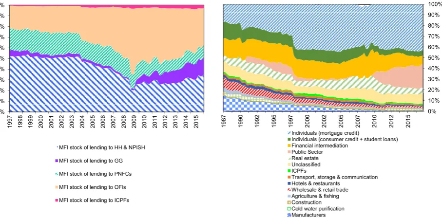
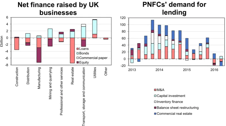
A quick glance at the financial position of MFIs vis-à-vis the rest of the economy confirms this (see Fig. 1, left panel). If we broaden the definition of MFI lending to include the purchase of shares, equity, and debt securities from non-MFIs, the figure shows that ‘lending’ to PNFCs is a small portion of ‘total lending’. The panel on the right shows MFI loans to non-MFI sectors. We can see that secured lending (mortgage loans) accounts for a big chunk of the total. If we take out lending to households, financial intermediaries and the public sector, the remaining (which represents lending to PNFCs) accounts for less than 40% during the 1990s, and less than 30% since 2010. Furthermore, as mentioned earlier, PNFCs might borrow to finance expenditures that would not count as investment, such as real estate, balance sheet restructuring, and the funding of mergers and acquisitions (Bank of England, 2016). Actual MFI lending for investment purposes might very well be below 20% of total MFI lending in the real world18.
17 With the exception of Jakab and Kumhof (2015)
18 These figures are for the UK, however, which is probably an extreme case. In Continental Europe banks play a more important role in the
14 Fig. 1. MFIlending to non-MFIs. The left panel shows financial assets held by MFIs (loans, debt securities, equity, shares, etc.), that have a liability counterpart in the borrowing sector. The right panel is restricted to lending in the form of loans, and breaks down private non-financial corporations (PNFCs) into sub-categories (e.g., construction, agriculture, etc.). MFI-to-MFI lending is consolidated out. Source: UK Office for National Statistics (left panel); Bank of England Bankstats (right panel)
Disaggregated data on bank lending makes it possible to disentangle lending that might contribute to GDP to different degrees. While a non-disaggregated view finds no strong causal relationship between credit flows and real activity19 (Zhu, 2011), the ‘funcionally differentiated’ perspective leads to much more conclusive and illuminating results. For example, Federal Reserve economists note that many contemporary ‘[a]nalysts have found that over long periods of time there has been a fairly close relationship between the growth of debt of the nonfinancial sectors and aggregate economic activity’ (BGFRS, 2013, p. 76). As shown by Bezemer and Hudson (2016) using their newly created dataset, in the US, growth of bank credit to the real sector and nominal GDP growth ‘moved almost one-on-one, until financial liberalisation gathered steam in the early 1980s’. Using cointegration analysis, Calza, Manrique and Sousa (2006) identified a long-run relationship linking loans to non-financial corporations and households and real GDP. While the authors argue that this should be interpreted as a long-run credit demand function, they concede that the inverse relationship, with credit supply driving GDP, cannot be excluded. In the Euro area, Ciccarelli, Maddaloni and Peydró (2010) find that a reduction of credit supply to firms significantly contributed to the decline in GDP growth. Shaikh (2016, pp. 704-5) shows that there is a strong correlation between the growth rate of nominal GDP and the growth rate of new purchasing power20 created by the banking sector relative to GDP. Regarding the direction of causality, Barnett and Thomas (2013) provide evidence of an independent role for bank credit shocks in influencing nominal output over and above aggregate demand shocks, stating: ‘credit supply shocks can account for most of the weakness in bank lending since the onset of the crisis and between a third and a half of the fall in GDP relative to its historic trend.’
19 ‘… tests of causality between credit and real activity are inconclusive concerning the direction of causality, or indeed whether causality
exists’ (Zhu, 2011)
20 New purchasing power is calculated as the sum of new domestic and foreign [bank] credit directed toward expenditure on GDP
transactions plus the current account balance of the external sector (Shaikh, 2016, p. 698) 0% 10% 20% 30% 40% 50% 60% 70% 80% 90% 100% 19 97 19 98 19 99 20 00 20 01 20 02 20 03 20 04 20 05 20 06 20 07 20 08 20 09 20 10 20 11 20 12 20 13 20 14 20 15
MFI stock of lending to HH & NPISH MFI stock of lending to GG MFI stock of lending to PNFCs MFI stock of lending to OFIs MFI stock of lending to ICPFs
0% 10% 20% 30% 40% 50% 60% 70% 80% 90% 100% 19 87 19 90 19 92 19 95 19 97 20 00 20 02 20 05 20 07 20 10 20 12 20 15
Individuals (mortgage credit)
Individuals (consumer credit + student loans) Financial intermediation
Public Sector Real estate Unclassified ICPFs
Transport, storage & communication Hotels & restaurants
15
However, when it comes to a disaggregated analysis of bank credit, the work of Richard Werner stands out as unique. While other authors skip over the role of banks as creators of the bulk of broad money, Werner’s analysis incorporates this fact explicitly as a critical element. Werner’s insight is that not only the uses of credit matter, but also the creditor, with an inescapable distinction to be made between creditors that lend out preexisting deposits and creditors that create new expenditure power ex nihilo when they lend. In other words, a proper analysis of credit calls for a distinction between bank lending and non-bank lending.
In the following I describe Werner’s theory and explore the literature that has contributed to it. The aim is to make the empirical and theoretical case for the existence of a stable, causal relationship between a component of credit (i.e., ‘bank credit for GDP transactions’) and nominal GDP.
2.2 The Quantity Theory of Credit and empirical evidence
Links between the ‘real’ and ‘monetary’ sides of the economy have long been acknowledged, the most common formulation being the ‘quantity equation of exchange’. This equation (Eq. (1)) gives a relationship between the money stock (M), the price level (P), the quantity of goods exchanged against money (Y), and the average turnover velocity of money (V).
M×V = P×Y (1)
The left-hand side shows the money stock M (measured in units of currency, e.g., £), multiplied by a factor V. The right-hand side shows the price level P (measured in £) multiplied by the quantity of goods exchange over the accounting period, for example a year (a flow, measured in £/year). The factor V has 1/year units, so both sides of the identity are consistent.
Rudimentary prototypical versions date back at least to the late 17th and 18th centuries, followed by increasingly sophisticated versions in the 19th and 20th century. For example, Locke, Hume, Smith, Thornton, Ricardo, Mill and Marshall employed the equation at one point or another in merely arithmetic or verbal form (Humphrey, 1984). Later Pigou (1917) gave it the form most widely known since then, (that of Eq. (1)), where P×Y represents nominal GDP (P being the GDP deflator), and M represents the money supply (measured as various monetary aggregates, e.g., M0, M1, M2, M3 or M4). Until about the mid-1980s, versions similar to Eq. (1) were the widely accepted work-horse that represented the link between the ‘real’ and the ‘monetary’ sides of the economy (Werner, 1997)
However, from the early 1980s onwards, faith in this link had been increasingly shaken by the widespread and growing empirical observation that velocity had become erratic, was declining significantly and the money demand function was unstable (e.g. Belongia and Chalfant, 1990; Boughton, 1991; Hendry, 1985). The ‘quantity equation’ relationship, expressed as a stable income velocity, ‘came apart at the seams during the course of the 1980s’ (Goodhart, 1989b). This phenomenon is known as the ‘velocity decline’. As a result, economists could not identify a reliable relationship between a monetary aggregate and nominal GDP. It was during this time that the paradigm of moneyless economic models became influential, which seemed to offer an scape route from an apparently intractable problem (Werner, 2012).
16
transactions21 (Werner, 2015)
The second of Werner’s innovations was to incorporate a definition of ‘money’ in line with the institutional realities of banking and money creation. In Werner (2012), he provides the reasoning: ‘nominal GDP growth this year means that more transactions (that are part of GDP) have taken place this year than last year … we know that this is only possible if more money has also exchanged hands to pay for these transactions … the next question therefore is: how can the amount of money used for transactions increase in our modern financial system?’ We know the answer: banks create 97% of the money supply of out nothing when they extend credit (see Section 1). Therefore, a proper definition of money should be ‘bank credit’. This excludes other types of debt contracts often referred to as ‘credit’, such as commercial paper or government bonds. Such instruments, as will be explained in the next section, will only count as bank credit if they are assets for the banks and liabilities for the non-banks22.
But despite deposits being created when bank credit is extended, loans and deposits are not the same thing. This is true both in a ‘practical’ sense and in a ‘quantitative’ sense. As for the first, as Werner (1997) eloquently points out:
‘Traditional money measures, such as M1, M2 or M3 mainly refer to money that is deposited with banks. At any moment in time, this is merely potential, not effective purchasing power, since deposits need to be withdrawn first. Deposits do not represent spending but the opposite, namely savings. But only spending can be expected to affect GDP directly’
Using total bank credit as the measure of the ‘money supply’ M in the equation has the advantage that credit always represents effective purchasing power, as no borrower will take out a loan if there is no plan to use the money for transactions. It also becomes possible to define effective purchasing power clearly—namely not bank liabilities, but bank assets or private sector liabilities to the bank sector (Werner, 1997). This overcomes the recurrent problem of how to define money properly23. Werner points out a third advantage, that disaggregated credit data are available by economic sector and hence provides a better tool to decompose the equation into different flows. However, the Bank of England has since begun to publish data on deposit holdings by economic sector (see the Bank of England’s Bankstats). Nonetheless, the first and second advantages still hold today.
As for the second aspect in which loans and deposits are not equal—namely that their quantities differ—, Werner (1996) showed that a broad credit measure, M2 + CD—traditionally used in Japan as a deposit measure—and a broad credit measure diverged greatly in the 1990s24. Fig. 2 shows a similar deviation for the case of the UK. While money and credit flows are tightly correlated, that relationship is not exact and at certain times credit growth has exceeded money growth. During these period, some of the lending to households and companies is likely to have been funded by issuance of non-deposit liabilities (for example long-term bonds, equity or securitisations) or deposits from non-residents (Bridges, Rossiter and Thomas, 2011).
21 Though this idea is not new, and already in the 1970s Milton Friedman considered such possibility; ‘Each side of this equation can be
broken into subcategories: the right-hand side into different categories of transactions and the left-hand side into payments in different form’ (Friedman, 1977, ‘Quantity Theory’, Encyclopedia Britannica, 15th edition, p. 435)
22 ‘… only the net creation of new transferable purchasing power is part of the definition. Thus what is often termed ‘credit’, for instance, the
issuance of corporate debt or government bonds, does not in itself constitute credit creation, as in these cases already existing purchasing power is transferred between parties’ (Werner, 2012)
23 Today, textbooks, as well as leading central bank publications, state that they do not know just what money is. In the words of then Federal
Reserve staff: “…there is still no definitive answer in terms of all its final uses to the question: What is money?” (Belongia and Chalfant, 1990, p. 32).
24 ‘While significant growth of M2+CD seemed to suggest an economic recovery in 1995, the credit aggregate suggested a contraction of
17 Fig. 2. Money and MFI credit flows. Both (broad) money (M4) and lending (M4L) flows exclude transactions with intermediate other financial corporations (OFCs) where available. M4L is adjusted to exclude the effects of securitisation. M4 covers private sector (households and companies, excluding public corporatios) holdings of sterling notes and coin, sterling deposits with banks and building societies, and sterling shares issued by building societies. Deposits are understood to include both certificates of deposit and other debt securities of up to and including five years’ original maturity issued by banks and building societies (Burgess and Janssen, 2007). The following identity holds: M4 = M4 lending + net foreign currency lending to private sector + net lending to public sector (including coin) + net lending to non-residents + net other assets. Source: Bridges, Rossiter and Thomas (2011)
Using the these two observations, two ‘surgeries’ can be performed on the quantity equation. First, the proper usage of ‘money’ as bank credit can be introduced (substituting M). Second, the decomposition of money flowing to two different types of transactions. Werner’s Quantity Theory of Credit is derived as follows:
CV = PQ (2)
CV = CRVR+CFVF (3)
PQ = PRQR+PFQF (4)
Eq. (1) shows the substitution of M (representing broad monetary aggregates) by C, which represents bank credit. Eq. (3) shows the decomposition of the flow of bank credit spent in the ‘real’ economy— on transactions that are part of GDP, such as investment or consumption—, and the flow that is spent in the ‘financial’ economy—primarily financial assets but also non-produced non-financial assets25 (e.g., real estate). The identity must also hold for the individual flows, so:
CRVR= PRQR= PRY with VR =PRY
CR = const.
CFVF= PFQF with VF =P QC F = const.
[image:18.595.190.408.89.268.2]18
Applying the chain rule for differences26—which, when applied to stocks, represent flows—, and using YoY relative growth rates:
ΔCR CR
=
Δ(PRY)
PRY (5) YoY ‘bank credit for GDP’ = YoY ‘nominal GDP’
ΔCF
CF
=
Δ(PFQF)
PFQF (6) YoY ‘bank credit for financ. trans.’ = YoY ‘financ. trans. volume’
This is Werner’s quantity theory, as presented in Werner (1992, 1995, 1997, 2005, 2015). Eq. (5) states that for a constant velocity VR, any percentage change in the stock of credit used for GDP transactions will translate one-for-one in a percentage change in nominal GDP. In other words, the stock of credit money that enters the real circulation determines the nominal value of goods and services. Eq. (6) states that for a constant velocity VF, any percentage change in the stock of credit used for non-GDP (or ‘financial’) transactions will translate one-for-one in a percentage change in the value27 (measured in nominal terms) of those transactions.
In the real world, the ‘two economies’ defined here are not hermetically shielded from one another, and their boundary is somewhat porous. Certainly, all analytical categories are human constructs, but they allow us to understand the world. Bank credit to the non-bank ‘asset’ sector, though it might ‘spill over’ to the the real sector eventually, does not enter the real sector initially to finance tangible capital formation or wages (Bezemer and Hudson, 2016). Its principal immediate effect is to inflate asset prices, specially non-produced assets such as real estate that are ‘in inelastic supply’ (Turner, 2014). Liang and Cao (2007) report that there exists unidirectional causality running from bank lending to property prices in China. Davis and Zhu (2011) on Hong Kong, and Goodhart and Hofmann (2003) on a panel of countries, find significant relationships between bank credit and property prices. Recent econometric analysis confirms that mortgage credit causes house prices to increase (Favara and Imbs 2014), and not just vice versa, as in the demand-driven textbook credit market theories. In this case, credit-money may also be used to purchase financial or real estate assets ‘without directly entering the investment-wage-consumption cycle of the real economy for a significant length of time’ (Werner, 1997).During the Great Moderation there were substantial asset price bubbles while the Consumer Price Index (CPI) or other standard measures of ‘real’ economy inflation were not much affected. As argued by Turner (2014a), there is no reason why asset price inflation will automatically translate—not even in the medium-to-long run—into goods and services inflation, contrary to what is believed. In some cases it will, it some cases it will not. Borio and Lowe (2004) note that in periods of low inflation and central banks commited to price stability, price pressures of unsustainable credit expansion ‘might take longer to emerge’. Instead, symptoms of the unsustainable boom would more likely first show up in excessive credit and asset price growth and hence in overstretched balance sheets, before showing up in consumer price inflation. Thus, in periods of price stability, the inflationary potential of excessive credit growth may be ‘camouflaged’ under the form of asset price overvaluation (Calza, Manrique and Sousa, 2006). Recognising this, The Bank of International Settlements (2016b, p. 20) recommends a more prominent role for monetary policy in preventing financial instability, allowing for the possibility of tightening policy even if near-term inflation appears under control. A case in which asset prices did not affect
26 Δ(ab) = aΔb + bΔa. With a constant, Δ(ab) = aΔb
27 The price of a product is defined as the value of one unit of that product. This price will vary directly with the size of the unit of quantity
19
consumer prices is Japan during the 1980s and early 1990s, when the proportion of bank loans that ended in real estate related transactions increased dramatically, resulting in nominal commercial land prices rocketing, while the economy registerd remarkably low consumer price inflation, as shown in Werner (1997). A case in which bank lending to the financial sector did enter the real economy was the UK during the 1980s. In this case, the speculators were mainly individuals, not firms. Their increased purchasing power reduced savings, boosted consumption and by entering the real circulation pushed up consumer prices (Werner, 1997).28
2.3 Empirical evidence and econometric tests supporting QTC
Since Werner formulated it in the 1990s, the ‘quantity theory of credit’ has been put to test by several authors with data for various countries (cf. Werner, 1997, 2005, 2014; Voutsinas and Werner, 2011; Ryan-Collins, Werner and Castle, 2016; Lyonnet and Werner, 2012; Bezemer and Werner, 2009). The theory has the advantage of making theoretical predictions that can be checked in the empirical data. On the other hand, it has the downside that it can never be refuted entirely conclusively. As two sides of the same coin, incompleteness for refutation implies incompleteness for corroboration. As I explain later, the variable ‘bank credit for GDP transactions’ is not, unlike monetary aggregates, directly observable, and empirical proxies have to be constructed that approximateit. This is further complicated by the fact that it is never possible to know whether the proxy one has constructed is the ‘correct proxy’, and a process of ‘triangulation’ is required, that is, the combination of theoretically-informed search with empirical refinement. Thus, the theory can only be granted shades of plausibility, and one must be equally judicious in the process of empirical testing as in the process of proxy construction. Issues related to proxy construction are explored in Sect. 3.
In the ‘fuzzier’ or more general formulation, the theory predicts the existence of a stable, autonomous mechanism linking two pairs of variables, with unidirectional causality going from the ‘bank credit’ variables to the ‘nominal value of transactions’ variables. In the case of the first pair of variables, causality runs from the growth rate of bank credit for GDP transactions to nominal GDP growth, which can be represented in the following form:
ΔCRb
CRb →
ΔnGDP nGDP
One of the implications of the existence of such autonomous relation is that, as an explanatory variable, bank credit for GDP transactions should outperform competing explanatory variables, where the variable to be ‘explained’ is nominal GDP growth. In fact, additional explanatory variables should be identified as redundant, and bank credit for GDP transactions should suffice (the ‘autonomous’ property). Another implication is that the direction of causality must run from bank credit for GDP transactions to nominal GDP. In its more precise formulation, the theory makes the prediction shown in Eq. (5), which reads: ‘there is a one-to-one relationship between the growth rate of nominal GDP and the growth rate of bank credit used for GDP transactions’. This prediction can be tested by checking the contemporaneous correlation between growth rates of the two variables. Importantly, it is not only correlation that matters, but the area between the two curves. That is, in growth rates, one variable should not be a scaled version of the other variable; both time series should appear to be, ideally, perfectly superposed one on top of the other.
What has the literature found so far regarding these predictions? As far as I know, there are seven
20
papers that try to test some aspect or other of the theory. These papers share a common methodology. First, they construct a proxy of ‘bank credit used for GDP transactions’, each with their own peculiarities but following the same overall logic29. Then various econometric tests follow, of the ‘general-to-specific’ (GETS) type (Hendry and Mizon, 1978), which consists of a single independent variable (nominal GDP growth), and and a number of candidate explanatory variables and their lags. These variables compete with each other in terms of explanatory power and significance. This equation is reduced based on progressive discarding of candidate variables based on statistical (in)significance, a sequential downward reduction, going from a general to a parsimonious equation. The competing variables often are a combination of a short term interest rate, a long-term interest rate, the growth rate of a broad monetary aggregate, ten-year bond yields, exchange rates, and the growth rate of the proxy of bank credit for GDP transactions. This method has the advantage of being inductive model-independent approach, with minimum or none a priori assumptions and restrictions (Ryan-Collins, Werner and Castle, 2016). The general-to-specific methodology has a good track record when it comes to estimating robust time series models (see e.g. Bauwens & Sucarrat, 2010; Voutsinas & Werner, 2010; Werner, 2005). The papers also perform various other tests, including Granger causality tests, strong exogeneity tests, etc.
Werner (1992, 1997, 2005) was the first to perform such tests for the case of Japan, followed by Voutsinas and Werner (2011b). They show that credit for GDP transactions explains nominal GDP well over several decades (‘growth of loans to the real economy single-handedly accounts for almost 90 % of nominal GDP growth in the observed time period’), while alternative explanatory variables—including interest rates and money supply—are eliminated in a reduction from a general to the parsimonious specific model (Hendry and Mizon, 1978). Explicit tests for omitted variables, adding M2+CD, ten year bond yields and exchange rates also found no omissions. Granger-causality is uni-directional from credit to growth at the 1% significance level, concluding that ‘bank credit growth appears to be in a stable long-term relationship with nominal GDP growth’.
Similarly, Lyonnet and Werner (2012) found that UK credit for GDP transactions explains nominal GDP over several decades, beating monetary aggregates, interest rates, central bank asset purchases and a variable representing ‘qualitative easing’ in a reduction from the general to the parsimonious form. The also find their proxy is ‘is found to be in a stable long-term relationship with nominal GDP growth’. Ryan-Collins, Werner and Castle (2016) and Lyonnet and Werner (2012) both construct proxies for the UK. Both sets of authors use Bank of England data. In both papers, the authors find a ‘long-run cointegrating relationship’ between the growth rate of nominal credit to the real economy and nominal GDP growth, discarding competing explanatory variables such as the bank rate, bank reserves, asset purchases by the Bank of England, the ratio of long-term assets of central bank balance sheet (‘qualitative easing’) and the money supply (M4), in a general-to-specific econometric model. Moreover, they find real economy credit growth to be strongly exogeneous to nominal GDP growth, in line with the results obtained by Barnett and Thomas (2013) on the independent role for bank credit shocks in influencing nominal output over and above aggregate demand shocks.
Bezemer and Werner (2009) study the link between credit and output in the Czech Republic, by using separate measures of credit to the real sector and credit to the financial sector. The authors find their ‘… disaggregated measure for credit flows exhibits better short-term correlation and causation to output growth than traditional, aggregate measures of credit and money. Our measure also appears to be a better annual predictor of nominal growth’.
Werner (2014) constructs a proxy for CRb for the Spanish economy using data from Banco de España (Bank of Spain) covering 1995-2013. The author finds that ‘bank credit for GDP transactions’ outperforms competing explanatory variables in a downward reduction from a general model to a
21
[image:22.595.78.515.188.340.2]parsimonious model, where the independent variable is nominal GDP growth. The competing variables are interest rates (10-year benchmark government bond yield) and money supply (M1). Co-integration and Granger-causality analysis in these studies suggests ‘unidirectional causation from bank credit creation to nominal GDP growth’.
Table 3 shows the estimated (inverse) velocities by the different authors. Given that the papers find a stable cointegrating relationship between nominal GDP growth and growth rate of the proxy, this velocit