Munich Personal RePEc Archive
Effect of aging on housing prices:
evidence from a panel data
Sun, Tianyu and Chand, Satish and Sharpe, Keiran
UNSW Canberra
1 November 2018
Effect of aging on housing prices: evidence
from a panel data
Tianyu Sun*, Satish Chand and Keiran Sharpe
Abstract:
We empirically test the effect of ageing on housing prices. Our analysis shows that a decline in the fertility rate and an increase in longevity – the two main causes of an ageing population
– have divergent effects on housing prices. This empirical finding helps us to reconcile a conflict which has lasted for 30 years in literature. We show that a decline in the fertility rate generally lowers housing prices because there are fewer workers in the population. At the same time, the workers and retirees react differently towards the impact of longer lifespans. In particular, the workers are urged to purchase more houses as a form of of saving and thus raise the prices, while the retirees tend to sell a greater fraction of the housing for extra funding. The conclusions correspond well with the Life Cycle Hypothesis and are drawn by using a semi-parametric method on an international panel data.
Keywords: Ageing, Fertility, Longevity, Housing prices, Semi-parametric analysis
JEL classifications: C14, E31, J11, R21
* Corresponding author.
Email-addresses: [email protected].
Introduction
Housing price dynamics are tightly related with households’ standard of living (Iacoviello 2011, Xie and Jin 2015); however, regarding the effect of demographic changes on housing prices, the literature gives mixed results. Researchers disagree over the importance of an aging population in influencing housing prices, and the research from both sides appear solid.For example, Mankiw and Weil (1989), Takáts (2012) and Essafi and Simon (2015) suggest an aging population has a significant effect on housing prices. In contrast, Engelhardt and Poterba (1991), Eichholtz and Lindenthal (2014) find that the effect is either insignificant or mixed. These contradictory views await further research to reconcile the conflict, and this paper will address this aim empirically.
In particular, we will test the theoretical argument brought up by Sun, Chand, and Sharpe (2018), who explicitly illustrate that the contradictory conclusions in the literature is caused by the divergent effect of fertility rate decline and longevity increase. It suggests that the fertility rate decline will lower the housing price because of a decline in the working population. Meanwhile, an increase in longevity will boost the price because the workers are more motivated to increase purchases. Note that the aging is caused by both the demographic changes above, thus it is possible that the contradictory empirical results noted above could come from the different nature of the fertility rate and longevity of their samples. This theoretical finding is also in line with the work of Takáts (2012).
The theoretical argument about, although reunite the conflicting views in literature, lacks empirical evidence for support and justification, and this paper fills this gap. By using a panel data of 19 advanced economies, we show that the worker population has a positive effect on housing prices, so the fertility rate decline would lower housing prices by reducing the worker population. This result is consistent with Choi and Jung (2016). In addition, our result
documents that a longer life expectancy would change the workers’ behaviour and urge them to purchase more housing assets for saving purposes, and thus an increase in longevity would boost the prices. Therefore, the justification of both sides is provided.
With regards to methodology, we first set up a simple model that has its origins in Takáts (2012). In this model, total population is divided into workers and retirees. Thus, their effects on house prices can be estimated separately. The data used in this estimate is from the Bank of International Settlement and the World Bank. It covers 19 advanced economies from 1970 to 2016. The international samples with a long sample period are more appropriate to identify the effects than using single countries (Takáts 2012).
The empirical result of the simple model confirms that the workers and retirees have significant and divergent effects on house prices. A one percent increase in worker population is associated with 1.62% higher house prices, and a one percent higher retiree population corresponds to around 0.81% lower house prices. This result indicates that if the worker population continues to rise then the house prices will follow in-step. Meanwhile, an increase in the retiree population will depress house prices, indicating that the motivation in selling houses overwhelms the demand increase of a larger retiree population. The divergent effects correspond well with the Life Cycle Hypothesis (LCH).
The opposing effects of worker and retiree population can be further investigated by extending the simple model. Here, this simple model is widened to allow the coefficients to be functions of life expectancy, the intention being to capture the behavioural changes that are caused by longevity increases. This is the benchmark model in this paper. Here, we argue that workers and retirees are sensitive to different aspects of life expectancy. Workers focus on the total length of expected lifespan because they need to plan their savings accordingly. Meanwhile, retirees are sensitive to growth rates of life expectancy so as to adjust their already existing life-cycle plans. The analysis on this difference is another distinct contribution of this paper that has not been identified by the previous research.
The empirical result of the benchmark model confirms that the effects of life expectancy are significant. The coefficient of workers is an increasing function with respect to the length of
life expectancy. Along with longevity increase, the value of workers’ coefficient has increased
The varying coefficients of the benchmark model are estimated by the Generalised Additive Model (GAM), and it forms another contribution of this paper. Although the GAM is widely used in the economic studies, especially the topics about housing prices1, it has generally been used to estimate the nonlinear impacts of explanatory variables on response variables. To the
best of the authors’ knowledge, our work is one of the first that uses this method on measuring the changes in coefficients in this area to reveal households’ behaviour. The result shows that the varying coefficient can be well consistent with the LCH. The novelty lies that the classic economic theories and the data-driving semiparametric methods can be embedded together as shown in this paper.
The remainder of this paper is organized as follows. The second section introduces the methodology. Specifically, a simple model is presented first and then extended to our benchmark model. The data and results are shown in the third section, while the fourth section tests the robustness of the key conclusions. The final section concludes.
1 See, for example, Martins-Filho and Bin (2005), Brunauer et al. (2010), Helbich (2015), and Rajapaksa et al.
Methodology
In this section, we introduce the model specifications used in this paper. More concretely, we adopt a simple model from the extant literature and then extend the simple model to incorporate life expectancy. This extension will be denoted as the benchmark model. The specifications and their economic meaning in behind will set the foundation for the rest of this paper.
Simple model
The simple model adopted in this research is a panel regression that is drawn from Takáts (2012), where the effect of population is highlighted and confirmed as a significant factor in determining house prices. In this paper, we divide the population into workers and retirees, while children are omitted for simplicity. Additionally, income is incorporated as another component in this regression for house prices, while the age structure as in Takáts (2012) is dropped because it can be represented by the worker and retiree population. The model specification is written as follows:
∆𝑙𝑛𝑃𝑖𝑡 = 𝛼 + 𝛽𝐼∆ ln 𝐼𝑛𝑐𝑜𝑚𝑒𝑖𝑡 + 𝛽𝑤∆ ln 𝑊𝑜𝑟𝑘𝑒𝑟𝑠𝑖𝑡+ 𝛽𝑟∆ ln 𝑅𝑒𝑡𝑖𝑟𝑒𝑒𝑠𝑖𝑡
+ 𝜙𝑡+ 𝜀𝑖𝑡 (1)
where P denotes real house prices, 𝛼 is the intercept, 𝑊𝑜𝑟𝑘𝑒𝑟𝑠 / 𝑅𝑒𝑡𝑖𝑟𝑒𝑒𝑠 denote the population of workers / retirees. Additionally, 𝜙 denotes the time fixed effect. Following Takáts (2012), this variable will capture factors that have global impacts, e.g. oil price shocks or global financial crisis. Subscript 𝑖 denotes country and subscript 𝑡 represents time (year).
As shown in Eq. (1), the variables are taken in natural logarithms first and then differenced. After implementing this procedure, the variables denote the percentage change of their original values. The direct reason of adopting these procedures, as stated in Takáts (2012), is to eliminate the unit root in the series, and this study will use the same strategy (see the section of data).
houses to fund their consumption. This difference should be reflected in the values of their coefficients, 𝛽𝑤 and 𝛽𝑟.
For the workers, the sign of coefficient 𝛽𝑤 should be positive because of their purchasing behaviour. However, we could not decide on the sign of 𝛽𝑟 (the coefficient of retirees), because multiple effects influence the value of this coefficient. On the one hand, the increase in the population of retirees will raise the demand for housing, thus the effect on house prices should be positive. On the other hand, the LCH indicates there will be stimulus for retirees to sell their houses, thus a negative effect could also be observed. In this study, until the results from empirical data are revealed, we cannot decide which one will be dominant.
The set-up of this simple model has two possible implications. Firstly, it fills an existing research gap. In Takáts (2012), the significance of total population is highlighted; however, we could not reach conclusions about the effects of different age groups. This paper will fill this gap by looking into the effects of workers and retirees on house prices separately. The values of the coefficients will reflect the influences from these two different age groups. Moreover, this simple model will set a foundation for its extension – the benchmark model – which is used to study the effect of longevity increase on house prices.
Benchmark model
The benchmark model will extend the simple model to have life expectancy incorporated. Specifically, the coefficients of workers and retirees will no longer be viewed as constants but as functions of life expectancy. We will analyse the theoretical meaning of this setting before providing the model specification. The analysis will provide insights into the relationship
between life expectancy and households’ life-cycle behaviour.
For workers, the coefficient 𝛽𝑤 (see Eq. 1) should be an increasing function with respect to life expectancy. According to the LCH, when workers have a longer life expectancy, they should purchase more houses as a means of saving (Sun, Chand, and Sharpe 2018). Consequently, house prices rise. If indeed true, then even if the worker population stays the same, house prices will rise accordingly when a longer lifespan is anticipated.
the expected lifespan. This argument is novel in literature because the previous studies neglect the fact that the retirees have already planned their lives when they are workers (ref). Consequently, retirees do not make plans according to the whole lifespan because a bulk of it (worker period) is already in the past. However, they can make decisions to change their existing plans. In particular, when the growth rate of life expectancy is positive, they should sell a greater fraction of the housing asset to fill the funding gap against the previous plan and thus drag down the price. From this perspective, the coefficient of retirees should be a decreasing function with respect to the growth rates of life expectancy.
The distinction between total length and growth rates of life expectancy is essential in identifying the effects of life expectancy on house prices. For example, a length of life expectancy, like 75 years, could correspond to either increasing or decreasing growth rates, and we do not know which one is true unless other information is provided. Similarly, a growth rate of life expectancy, like 1%, can reveal no information on the length of life expectancy. Thus, although they are both concerned with life expectancy, they denote different economic meanings and should not be conflated. For the reasons above, the rest of this paper will use variable 𝑙 / ∆𝑙 to denote the length / growth rates of life expectancy, and the specification of the benchmark model is as follows:
∆𝑙𝑛𝑃𝑖𝑡 = 𝛼 + 𝛽𝐼∆ ln 𝐼𝑛𝑐𝑜𝑚𝑒𝑖𝑡+ 𝛽𝑤(𝑙𝑖𝑡)∆ ln 𝑊𝑜𝑟𝑘𝑒𝑟𝑠𝑖𝑡
+ 𝛽𝑟(∆𝑙𝑖𝑡)∆ ln 𝑅𝑒𝑡𝑖𝑟𝑒𝑒𝑠𝑖𝑡+ 𝜙(𝑡) + 𝜀𝑖𝑡 (2)
Here, we care about that whether the function 𝛽𝑤(𝑙) is an increasing function with respect to life expectancy, and whether the value of function 𝛽𝑟(∆𝑙) will vary when growth rate changes.
Additionally, the time fixed effect 𝜙 in the simple model will also be treated as a function of time in the GAM method, i.e. 𝜙(𝑡).
The extant literature suggested that we can use questionnaires to collect data of people’s
subjective life expectancies2. However, by no mean can we be back-casted to 1970s to conduct this data collection on households to reveal their subjective life expectancy at that time. Meanwhile, the Human Mortality Database3 has provided estimations of households’ life expectancies by age based on mortality rates. However, the estimations about workers' life expectancies in this dataset do not have material difference comparing with the current data. Thus, for simplicity of discussion, we will use the life expectancy at birth as the life expectancy of workers.
In this paper, we will use generalized additive model (GAM) to estimate these coefficient functions of the benchmark model. As a semiparametric econometric method, it can estimate flexible model specifications, including cases that coefficients are functions of other factors. Therefore, this method could unveil richer patterns of association between response and explanatory variables, and thus outperform naive parametric and polynomial models (Martins-Filho and Bin 2005, Pace 1998). Regarding house prices, studies using this method have focused on the determinants of house prices (see footnote 1), and the discussion of this research shows that this method can be well applied on the economic studies.
In a manner which differs from the bulk of the literature that assumes the explanatory variables have non-linear impacts on house prices directly, we argue that the impact could be brought about by changing the coefficients of explanatory variables. In particular, we suggest that longevity could affect house prices through the channel of changing households’ behaviours, and the changes are captured by the coefficient changes as discussed in previous paragraphs. In this way, we show that the semiparametric regression method can be applied not only to the fields that are uncovered by the classic economic theories but also extending the understanding of these theories. For our study, we show that the GAM can be well embedded with the LCH, and it is one of the first that starts this direction.
One question may arise regarding the choice of the methodology. Why don’t we treat lifespan and its growth rates as independent variables as income? If we were to do so, the results could be analysed by the traditional econometric method. The reason that we choose the semiparametric regression method, as has been discussed above, is that the effect of longevity changes should be reflected by the changes of households' behaviours. Treating lifespan
Data and Results
Data
There are two datasets used in this paper. The first dataset providing house prices is from the Bank of International Settlement4 (BIS). This dataset contains 23 countries or areas. We use data from 19 advanced economies. They are Australia, Belgium, Canada, Switzerland, Germany, Denmark, Spain, Finland, France, the United Kingdom, Ireland, Italy, Japan, Korea, Netherlands, Norway, New Zealand, Sweden, and the United States.
We use the advanced economies because: 1) they have longer data series, and 2) the economy operations are more stable. A longer data series is preferred in an empirical study, and stable economy operations imply fewer policy shocks on house prices, so we can focus on the effects of demographic changes. This dataset is an intersection of the conditions above, and thus is suitable for this research.
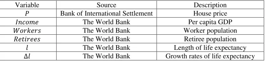
Besides house prices, which is denoted by the variable 𝑃, all other data is from dataset of the World Bank5. According to the World Bank, workers are people aged from 15-64, and retirees are the ones aged above 64. This study will use the same definitions, and the population of them are denoted by the variables 𝑊𝑜𝑟𝑘𝑒𝑟𝑠 and 𝑅𝑒𝑡𝑖𝑟𝑒𝑒𝑠 respectively. In addition, the length of life expectancy 𝑙 that was discussed in the methodology section will be represented by the life expectancy data in this dataset. Meanwhile, changes in life expectancy ∆𝑙 will be calculated based on the same data. Lastly, the variable 𝐼𝑛𝑐𝑜𝑚𝑒 is used to denote the per capita GDP in real terms. The variables, together with their sources and descriptions, are listed in Table 1. Following Takáts (2012), the house prices are used in their real terms and adjusted by the CPI.
As illustrated in the methodology section, we use log difference operation to avoid the unit root in the data, and the Levin-Lin-Chu unit root test (Levin, Lin, and James Chu 2002) is adopted for the examination of results. The test results are provided in Table 26. As we can see, the
4 Source: National sources, BIS Residential Property Price database (http://www.bis.org/statistics/pp.htm).
Download date: 08 August 2018
5 Per capita GDP: https://data.worldbank.org/indicator/NY.GDP.PCAP.KN;
Population ages 15-64 (% of total): http://data.worldbank.org/indicator/SP.POP.1564.TO.ZS; Population ages 65 and above (% of total): http://data.worldbank.org/indicator/SP.POP.65UP.TO.ZS; Population, total: http://data.worldbank.org/indicator/SP.POP.TOTL;
Life expectancy at birth, total (years): http://data.worldbank.org/indicator/SP.DYN.LE00.IN; Download date (all): 08 August 2018
Population of workers, population of retirees, and changes in longevity are calculated by author.
original data and the log levels cannot reject the null hypothesis of having unit roots. Nevertheless, the log differenced data shows strong rejection on the existence of the unit root (see Table 2). Here, the log difference of retiree population is intercept stationary, and the intercept is caused by the aging population. For an aging population, the growth rates of the retiree population are positive rather than stable around zero. Note that the log difference operation calculates the growth rates of a variable, thus the positive growth rates of retiree population bring about the intercept of the test.
Table 1 Source and Description of the Variables
Variable Source Description
𝑃 Bank of International Settlement House price
𝐼𝑛𝑐𝑜𝑚𝑒 The World Bank Per capita GDP
𝑊𝑜𝑟𝑘𝑒𝑟𝑠 The World Bank Worker population
𝑅𝑒𝑡𝑖𝑟𝑒𝑒𝑠 The World Bank Retiree population
𝑙 The World Bank Length of life expectancy
∆𝑙 The World Bank Growth rates of life expectancy
Table 2 Levin-Lin-Chu Unit-Root Test
original data log levels log difference
House prices >0.999 >0.999 <0.001
Per capita GDP 0.9893 >0.999 <0.001
Population of Workers 0.9999 0.9997 <0.001
Population of Retirees >0.999 >0.999 <0.001
Note: the tests are computed with the purtest function from package plm-1.5-67. The null hypothesis is
that the data has a unit root, and the numbers are the possibility of having the unit root. The log
[image:12.595.69.535.566.670.2]difference of the population of retirees is intercept stationary.
Table 3 Statistic information of the data (from 1971 to 2016)
Description Min 1st quartile Median 3rd quartile Max Std. Observations
House prices -0.244 -0.024 0.020 0.061 0.299 0.075 858 Per capita GDP -0.091 0.008 0.020 0.033 0.218 0.025 858 Population of Workers -0.019 0.003 0.006 0.011 0.048 0.007 858 Population of Retirees -0.023 0.012 0.019 0.027 0.057 0.012 858 Life Expectancy -0.007 0.001 0.003 0.004 0.016 0.003 858
Note: these are growth rates of these variables, source from author calculation.
The statistic information of this log differenced data is shown in Table 3. Here, we show the quartiles of the annual growth rates of these variables. For all the variables, the minimum values of growth rates are negative, while the 1st quartile values of them are positive. This characteristic means that the dataset covers diversified situations (because both the negative and positive signs are included), while the variables have positive growth rates in most of the years.
In Table 3, note that the population of retirees has higher growth rates than that of workers in all the quartiles, implying an aging population in these countries. Meanwhile, the house prices have the largest fluctuations among these variables, while longevity has the smallest standard deviation among all variables. Will life expectancy – a variable with small variations – have significant effect on house prices? An answer to this question will be left to the result sections.
[image:13.595.91.500.509.699.2]In addition, a histogram of life expectancy is shown in figure 1. Note that only a small fraction of observations has life expectancy lower than 70, while the majority are above that. In fact, only 12 of 858 observations are with a life expectancy below 70, indicating that the number may be insufficient to detect effects of longevity within this range. Insufficient observations imply that the conclusion lacks statistical power (Chipman 1964) and sometimes could be influenced by other factors. For example, all the 12 observations (that life expectancy less than 70) are of Korea from 1975-1987. In this period, it is the land policy of South Korea that significantly affected house prices (Hannah, Kim, and Mills 1993).
Figure 1 Histogram of Life Expectancy Life Expectancy
F
re
q
u
e
n
cy
60 65 70 75 80 85
0
50
100
Results of the Simple Model
The results of simple model are listed in Table 4. The result of the Hausman test suggests that the fixed effect model should be used in the regression. In addition, the result of the Lagrange Multiplier Test shows that the time fixed effect is significant. Thus, the regression specification of Eq. (1) that captured these features can be used in this study.
The panel regression analysis shows that all the selected variables are significant at the 1% level (see Table 4). The coefficient signs of worker and retiree population are opposite to each other, indicating that these two age groups have opposite impacts on house prices. Specifically, the impact of worker population is positive, while the impact of retiree population is negative. Furthermore, the coefficient sign of income is positive.
Next, we have a closer look into the coefficient values and discuss their economic meanings. The coefficient value of per capita income is 1.16. Thus, when per capita income rises 1%, the corresponding house prices will also rise about 1%. For the workers, the coefficient value is 1.62, indicating that if worker population increase by 1%, house prices will rise 1.62% ceteris paribus. Thus, the house prices will rise faster than the worker population. For retirees, the parameter value is -0.8, implying an increase in retirees’ population will lead to a decline in
house prices.
Table 4 Results of the Simple Model
Term Estimate Std. Error t value Pr(>|t|)
Income 1.168 0.102 11.421 < 2.2E-16***
Worker 1.621 0.332 4.871 1.33E-06***
Retiree -0.805 0.2064 -3.987 7.26E-05***
R-squared: 0.176
Results of the Hausman test: Chisq = 57.637, p-value = 1.879e-12
Lagrange Multiplier Test - time effects (Breusch-Pagan) for unbalanced panels: p-value < 2.2e-16
Note: The estimates are computed with the plm function from package plm-1.5-6. The
null-hypothesis of Hausman test is that random effect model is preferred, and a rejection indicates that fixed
effect model should be used. The null-hypothesis of time effect test is that there is no time fixed effect, and a rejection indicates that time fixed effect model is preferred.
𝐼𝑛𝑐𝑜𝑚𝑒 ∙ 𝑃𝑜𝑝𝑢𝑙𝑎𝑡𝑖𝑜𝑛 = 𝐻𝑜𝑢𝑠𝑒 ∙ 𝑃𝑟𝑖𝑐𝑒 (3)
This equation implies no consumption and all wealth is held in the form of housing. Although it is a great simplification of reality, we may compare the conclusions of this equation to the results of our simple model in order to secure an intuitive grasp of the correlations.
In Eq. (3), when per capita income increases by 1%, the house prices should increase by 1% ceteris paribus. This conclusion is consistent with the coefficient value of income in the simple model. In addition, if per capita income and house supply are constant, then a 1% increase in population should result in 1% rise in house prices. If we divide total population into workers and retirees, what will happen then? We first assume that the two age groups have the same behaviour. In this situation, an increase in worker population or retiree population should have the same effect on house prices, and both the coefficient values should be 1.
However, this conclusion from Eq. (3) contradicts the regression results in Table 4. The regression results show that the coefficient value of workers / retirees is higher / lower than 1. Thus, we could conclude that the behaviours of workers and retirees are different. This behavioural difference can be explained according to Life Cycle Hypothesis (LCH). This theory suggests that workers will purchase more houses as a saving to fund their consumption in retired life. Thus, the coefficient value of workers should be higher than 1. Meanwhile, the retirees will sell their houses in retirement according to LCH. Therefore, the coefficient value of retirees should be lower than 1. These predictions from LCH corresponds well with the regression results (see Table 4).
Nevertheless, two questions cannot be answered by this simple model. The first one relates to the negative sign of the coefficient of retirees. Note that for retirees, there are two motivations that could affect house prices. On one hand, the retirees will sell their houses to support their consumption. This motivation will depress house prices. On the other hand, an increase in retiree population could result in higher demand for housing, and so then raise the prices. The parameter value of retirees is determined by the net effect of both sides. In the regression results, a negative sign of this parameter indicates that the selling behaviour outweighs the other. The question then is: is there a factor influencing the weight of this selling behaviour?
will deepen our understanding about the interaction of house prices and households’ behaviours.
This discussion will be left to the following section.
Results of the Benchmark Model
As mentioned in section of Methodology, the benchmark model is an extension of the simple model. Thus, the results of the benchmark model will not only incorporate the ones of the simple model, but they could also answer the questions unsolved in the previous section.
The results of the benchmark model can be divided into that of the linear / non-linear terms according to Eq. (2). The results of linear terms are shown in Table 5. As we can see, the income is significant at 1% level, and the coefficient value of income is 1.23, indicating that a 1% increase in income would result in about 1% increase in house prices. This result is similar to that of the simple model. The intercept term will be viewed as influences from unknown characteristics (Bates, Kahle, and Stulz 2009).
The results of non-linear terms are shown in Table 6. The first column in Table 6 shows the corresponding terms in Eq. (2): the coefficient of workers, the coefficient of retirees, and the time specific effects. The results of these terms are fitted functions, and thus we cannot present their values directly. Instead, four indicators are shown.
Table 5 Results of the Benchmark Model: Linear Terms
Estimate Std. Error t value Pr(>|t|)
(Intercept) -0.00852 0.00499 -1.706 0.0884*
Income 1.237 0.0929 13.312 <2.00E-16***
Table 6 Results of the Benchmark Model: Non-Linear Terms
K EDF F P-value
βw(l) ∙ Worker 10 2.558 11.463 1.37E-06***
βr(∆l) ∙ Retiree 10 2 10.597 2.84E-05***
ϕ(t) 9 8.509 9.852 2.90E-14***
R-squared: 0.305
Note: The estimates are computed with the gam function from package mgcv-1.8-248.
The first indicator, K, denotes the maximum degree of freedom allowed for these terms. This setting is necessary because of the need to trade-off between the complexity and fitting performance. Theoretically, we can use highly non-linear functions to fit the data, but this
complexity will be meaningless if we cannot conclude anything from the result. Although algorithms in software can select a maximum degree automatically9, this selection is driven by the number of observations instead of the nature of a study. Thus, manual selection of K should be plausible when insights of a study are blocked (Wood 2017).
The second indicator, EDF, denotes the estimated degree of freedom of the fitted function. After choosing the maximum degree of freedom K, algorithms in software can conduct the fitting automatically. Moreover, the algorithms will choose an EDF (< K) automatically as the best trade-off between complexity and fitting performance.
The third indicator is F statistic values. By comparing the model performance with and without a term, we could reach conclusion about the importance of this term. This importance is measured numerically by the F statistic value. Furthermore, the fourth indicator, P-value, will give the probability that a term is zero (under the F statistic value). Thus, a small P-value (e.g. less than 1%) will indicate that this term is significant (at 1% level).
Specifically, all the non-linear terms are significant at 1% level (see Table 5-6). The maximum degree of freedom (K) of these terms are selected automatically: for the coefficient of workers, 10; for the coefficient of retirees, 10; and for the time specific effects, 9. After calculation, the
EDF of workers’ coefficient is shown as 2.558, indicating this coefficient could be a non-linear function of life expectancy (see figure 2). Similarly, the EDF of retirees’ coefficient is 2, and this result implies that a linear function (of growth rates of longevity) could explain the changes of this coefficient (see figure 3). Lastly, the time specific effects have an EDF as 8.509, showing that this time-related fluctuation is highly non-linear.
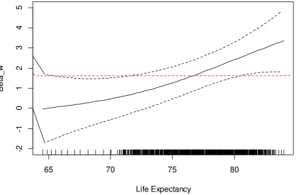
Next, we will focus on the figure 2 to examine the properties of the coefficient of workers,
𝛽𝑤(𝑙). As we can see, the coefficient is shown as an increment function with respect to life
expectancy, and this result corresponds well with the theoretical prediction. In particular, the function value increases along with the rises of life expectancy from lower than 1 to over 2. Here, the function values that lower than 1 could be influenced by the insufficient data when life expectancy is lower than 70 (see the discussion in the data section), and it will be further examined in the section of robustness checks.
9 The detail algorithms of this software can be found in Hastie and Tibshirani (2004), Wood (2003), Wood (2004),
Recall that we have estimated the 𝛽𝑤 as 1.62 in the simple model (see Table 4). This value has been highlighted in the horizontal (red) dash line in figure 2. As could be noticed, this dash line is around the average of the coefficient function. Thus, although the 𝛽𝑤 in the simple model (as a constant) could be the best estimation of this parameter, this estimation fails to capture its changes over different life expectancies. The benchmark model solves this problem and shows that the coefficient of workers is an increment function of life expectancy.
[image:18.595.91.510.329.604.2]Consequently, if worker population increases, the growth rate of house prices will be accelerating as life expectancy increases. This result indicates that, for workers, the motivation to purchase houses as a saving will get stronger when they predict a longer lifespan. Because the life expectancy continues rising in the context of a rapid peaceful development over the past several decades, the saving motivation of workers has been continually strengthened.
Figure 2 Workers’ Coefficient: A Function of Life Expectancy
Note: The continuous line shows the estimate of the smooth; the dashed lines represent 95%
confidence bands. The horizontal (red) dash line is the estimated value of this coefficient in the
simple model.
65 70 75 80
-2
-1
0
1
2
3
4
5
Life Expectancy
B
e
ta
_
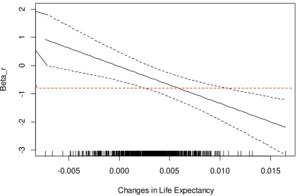
Figure 3 Retirees’ Coefficient: A Function of Changes in Life Expectancy
Note: The continuous line shows the estimate of the smooth; the dashed lines represent 95%
confidence bands. The horizontal (red) dash line is the estimated value of this coefficient in the
simple model.
Here, we want to further discuss the social meaning of this result. Note that when the coefficient
𝛽𝑤 > 0, an increasing worker population will push the house prices up. This price rise will
make it harder for the following worker generations to purchase houses. When it becomes increasingly difficult for younger generations to get into the housing market, this phenomenon will become a social problem – as is happening now in many countries (Metcalf 2018). Specifically, the result of benchmark model shows that 𝛽𝑤(𝑙) could be higher than 2, and this will make the price rising even quicker.
The coefficient change of retirees is shown in figure 3. In a manner different from that of workers, the coefficient of retirees is shown to be a function of growth rates of life expectancy. With a higher growth rate, this coefficient value will decrease accordingly. Recall that we have estimated the coefficient 𝛽𝑟 as -0.8 in the simple model (see Table 4). This value is denoted by horizontal (red) dash line in figure 3. It positions in the middle of the coefficient function as the case of workers. This result implies that this estimated value in the simple model is an average of the coefficient function in the benchmark model. From this perspective, the
-0.005 0.000 0.005 0.010 0.015
-3
-2
-1
0
1
2
Changes in Life Expectancy
B
e
ta
_
benchmark model shows more information than that of the simple model, especially in capturing the coefficient changes.
More concretely, when the growth rate of longevity is 0, the corresponding coefficient 𝛽𝑟(0) is about 0 (see figure 3). This result implies that, when longevity remains the same, the increase of retiree population will have little impact on house prices. In this case, the upward force from retiree population increase is about equal to the downward force from selling houses by retirees. In addition, when the growth rate of life expectancy is positive / negative, the sign of this coefficient would be negative / positive (see figure 3). From the perspective of LCH, when longevity decreases, retirees will sell less houses because their funding is more than planned in this situation. However, when longevity increases, retirees will sell a greater fraction of houses than expected to fund their consumptions. Therefore, this result is consistent with the LCH.
In sum, the benchmark model as an extension of the simple model has advantages in the following aspects. First, because the specification of the benchmark model is flexible (for example, the coefficient of workers is a function instead of a constant), it can fit the data better, and thus has a higher R-square (see Table 4 and 6). Second, the benchmark model makes the simple model a special case of it (see figure 2 and 3). Third, the benchmark model provides
links among house prices, life expectancy and households’ life-cycle behaviours. Specifically, the results of the benchmark model show how life expectancy affects house prices, and these influences are explained from the perspective of LCH. Lastly, the results of the benchmark model support the conclusion of the previous paper that a longer life expectancy of workers raises house prices. Moreover, it extends the analysis to retirees and provides clues on how longevity changes can affect their housing decisions.
Further Discussion
In this section, we further illustrate why we do not treat lifespan and its growth rates as independent variables as income. To answer this question, we provide an alternative model specification. In this specification, the lifespan and its growth rates are viewed as independent variables. In particular, the regression follows the following specification:
∆𝑙𝑛𝑃𝑖𝑡 = 𝛼 + 𝛽1∆ ln 𝐼𝑛𝑐𝑜𝑚𝑒𝑖𝑡+ 𝛽2𝑙𝑖𝑡+ 𝛽3∆𝑙𝑖𝑡+ 𝛽4∆ ln 𝑊𝑜𝑟𝑘𝑒𝑟𝑠𝑖𝑡
+ 𝛽5∆ ln 𝑅𝑒𝑡𝑖𝑟𝑒𝑒𝑠𝑖𝑡+ 𝜙(𝑡) + 𝜀𝑖𝑡 (4)
We present the results in Table 7 as follows:
Table 7 Results of the Alternative Model
Term Estimate Std. Error t value Pr(>|t|)
Income 1.330 0.105 12.623 < 2.2E-16***
Worker 2.151 0.343 6.264 6.07E-10***
Retiree Lifespan (Length) Lifespan (Growth Rates)
-0.806 0.00614
-2.928
0.202 0.00149
0.862
-3.977 4.121 -3.3932
7.60E-05*** 4.15E-05*** 7.24E-04***
R-squared: 0.207
Note: The estimates are computed with the plm function from package plm-1.5-6.
In the results of the alternative model, the estimated coefficients as well as their significance levels do not have material differences comparing with that of the simple model (see Table 4 and 7). In particular, the lifespan is shown to have significant positive effect on housing prices, while the growth rates of the lifespan would impact the housing prices negatively. This result corresponds well with the conclusions revealed by the benchmark model.
However, in the alternative model, even if we know that the lifespan and its changes could have opposite impacts on the housing prices, we do not know the specific mechanism causing the impacts. In contrast, our benchmark model provides the clues. The result shows that the
Robustness check
According to Lu and White (2014), our benchmark model could have suffer from misspecification because of endogeneity problems or omitted variables. Furthermore, the results could vary due to changes in sample periods or country selections. In this section, we present robustness checks against these possible drawbacks.
First, we follow Essafi and Simon (2015) to use lagged explanatory variables instead of the contemporaneous ones. This method precludes the possible endogeneity problems (Arellano and Bond 1991). In particular, the regression that is modified from the equation (2) is as follows:
∆𝑙𝑛𝑃𝑖𝑡 = 𝛼 + 𝛽𝐼∆ ln 𝐼𝑛𝑐𝑜𝑚𝑒𝑖,𝑡−1+ 𝛽𝑤(𝑙𝑖,𝑡−1)∆ ln 𝑊𝑜𝑟𝑘𝑒𝑟𝑠𝑖,𝑡−1
+ 𝛽𝑟(∆𝑙𝑖,𝑡−1)∆ ln 𝑅𝑒𝑡𝑖𝑟𝑒𝑒𝑠𝑖,𝑡−1+ 𝜙(𝑡) + 𝜀𝑖𝑡 (5)
, and we denote this alternative model as M1.
Secondly, the housing prices could be influenced by interest rates. Here, we use the interest rates of government bonds that mature in ten years to represent this variable. Choosing the long-term interest rate is warranted because buying houses is also a long-term investment and could be influenced by alternative investment choices. Here, the interest rate is source from the OECD10, and the regression model has the specification as follows:
∆𝑙𝑛𝑃𝑖𝑡 = 𝛼 + 𝛽𝐼∆ ln 𝐼𝑛𝑐𝑜𝑚𝑒𝑖𝑡+ 𝛽𝑤(𝑙𝑖𝑡)∆ ln 𝑊𝑜𝑟𝑘𝑒𝑟𝑠𝑖𝑡
+ 𝛽𝑟(∆𝑙𝑖𝑡)∆ ln 𝑅𝑒𝑡𝑖𝑟𝑒𝑒𝑠𝑖𝑡+ 𝐼𝑛𝑡𝑒𝑟𝑒𝑠𝑡𝑖𝑡+ 𝜙(𝑡) + 𝜀𝑖𝑡 (6)
, and this alternative model is denoted as M2.
Thirdly, the economic crisis from 2007 could have had influences on the estimation results because of its weighty impacts. Therefore, an alternative sample period, 1970-2006, is chosen to exclude the impacts of this event, and this model is denoted by M3. Lastly, we omit Korea as an example to check if the results would vary by country selections (M4). Korea is chosen because it becomes an advanced economy later than the other countries in our country samples.
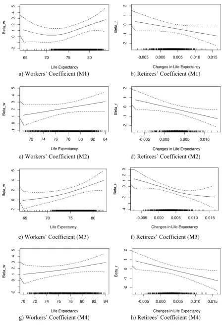
For all the alternatives above, the workers’ coefficient 𝛽𝑤 shows as an increase function when life expectancies are more than 70. In particular, the coefficient 𝛽𝑤 increases from about 1 to
over 2 in M2 and M4 (see figure 4c, g). The same pattern may be blurred in the results of the M1 and M3 (see figure 4a, e) because of insufficient observations whose life expectancies are lower than 70 (see the data section). Similarly, the coefficient of retirees 𝛽𝑟 is shown to be a decreasing function with respect to the changes in life expectancy in all the cases. In addition, when the changes in life expectancy are zero, the values of the coefficient 𝛽𝑟 are also close to zero, suggesting that the plans of retirees remain unchanged. Therefore, the non-parametric terms of our benchmark model are robust with the checks.
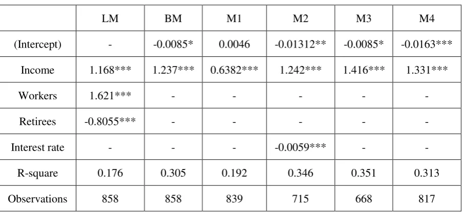
Table 8 Results of parametric coefficients
LM BM M1 M2 M3 M4
(Intercept) - -0.0085* 0.0046 -0.01312** -0.0085* -0.0163***
Income 1.168*** 1.237*** 0.6382*** 1.242*** 1.416*** 1.331***
Workers 1.621*** - - - - -
Retirees -0.8055*** - - - - -
Interest rate - - - -0.0059*** - -
R-square 0.176 0.305 0.192 0.346 0.351 0.313
Observations 858 858 839 715 668 817
Note: ***, **, * indicate significant at 1%, 5% and 10%. For the LM, the estimates are
computed with the plm function from package plm-1.5-6. For the rest of the models, the
estimates are computed with the gam function from package mgcv-1.8-24. In M2, we use the
differences in long term interest rates and the data is from the OECD data11.
Table 9 Results of non-parametric terms
BM M1 M2 M3 M4
𝛽𝑤(𝑙) 2.558*** 3.157*** 2.000*** 2.596*** 2.163***
𝛽𝑟(∆𝑙) 2.000*** 2.000** 2.000** 2.725*** 2.000*
s(Year) 8.509*** 8.484*** 8.689*** 8.671*** 8.571***
Note: the values denote the degree of freedom of the fitted function. Symbols***, **, * indicate
significant at 1%, 5% and 10%. To show clear patterns, the maximum degree of freedom of the
coefficient 𝛽𝑟 in M1 and M3 is restricted as 3 and 4 respectively, while the other settings are
kept the same as in the benchmark model.
[image:24.595.67.527.415.521.2]
a) Workers’ Coefficient (M1) b) Retirees’ Coefficient (M1)
c) Workers’ Coefficient (M2) d) Retirees’ Coefficient (M2)
e) Workers’ Coefficient (M3) f) Retirees’ Coefficient (M3)
[image:25.595.76.529.67.730.2]g) Workers’ Coefficient (M4) h) Retirees’ Coefficient (M4)
Figure 4 Robustness checks on the coefficients of workers and retirees
65 70 75 80
-2 0 1 2 3 4 5 Life Expectancy B e ta _ w
-0.005 0.000 0.005 0.010 0.015
-2
-1
0
1
2
Changes in Life Expectancy
B
e
ta
_
r
72 74 76 78 80 82 84
-1 0 1 2 3 4 5 Life Expectancy B e ta _ w
-0.005 0.000 0.005 0.010
-2
-1
0
1
2
Changes in Life Expectancy
B
e
ta
_
r
65 70 75 80
-2 0 2 4 6 Life Expectancy B e ta _ w
-0.005 0.000 0.005 0.010 0.015
-4 -2 0 1 2 3
Changes in Life Expectancy
B
e
ta
_
r
70 72 74 76 78 80 82 84
-2 0 1 2 3 4 5 Life Expectancy B e ta _ w
-0.005 0.000 0.005 0.010 0.015
-2
-1
0
1
2
Changes in Life Expectancy
B
e
ta
_
Before reaching our conclusion, we will present counterfactual tests on the model specifications. Recall that we have illustrated that it is different aspects of life expectancy which affect the behaviour of workers and retirees. For workers, it is the length of life expectancy that stimulates their purchasing behaviour. For retirees, different growth rates of life expectancy will influence the selling of their houses12. Here, we will present counterfactual tests to see what will happen if we substitute the ones with another.
Specifically, we suggest three alternative specifications as following:
∆𝑙𝑛𝑃𝑖𝑡 = 𝛼 + 𝛽𝐼∆ ln 𝐼𝑛𝑐𝑜𝑚𝑒𝑖𝑡 + 𝛽𝑤(𝑙)∆ ln 𝑊𝑜𝑟𝑘𝑒𝑟𝑠𝑖𝑡
+ 𝛽𝑟(𝑙)∆ ln 𝑅𝑒𝑡𝑖𝑟𝑒𝑒𝑠𝑖𝑡+ 𝜙(𝑡) + 𝜀𝑖𝑡 (7)
∆𝑙𝑛𝑃𝑖𝑡 = 𝛼 + 𝛽𝐼∆ ln 𝐼𝑛𝑐𝑜𝑚𝑒𝑖𝑡+ 𝛽𝑤(∆𝑙)∆ ln 𝑊𝑜𝑟𝑘𝑒𝑟𝑠𝑖𝑡
+ 𝛽𝑟(∆𝑙)∆ ln 𝑅𝑒𝑡𝑖𝑟𝑒𝑒𝑠𝑖𝑡+ 𝜙(𝑡) + 𝜀𝑖𝑡 (8)
∆𝑙𝑛𝑃𝑖𝑡 = 𝛼 + 𝛽𝐼∆ ln 𝐼𝑛𝑐𝑜𝑚𝑒𝑖𝑡+ 𝛽𝑤(∆𝑙)∆ ln 𝑊𝑜𝑟𝑘𝑒𝑟𝑠𝑖𝑡
+ 𝛽𝑟(𝑙)∆ ln 𝑅𝑒𝑡𝑖𝑟𝑒𝑒𝑠𝑖𝑡+ 𝜙(𝑡) + 𝜀𝑖𝑡 (9)
In the first case, both coefficients 𝛽𝑤 and 𝛽𝑟 are affected by length of life expectancy. In the second case, the coefficients are functions of growth rates of life expectancy. In the third case, the positions of two variables are switched, i.e. growth rates of life expectancy will influence the workers, while the retirees focus on the total length. The three alternative specifications above are indexed as M5, M6 and M7 respectively, and the results are shown in the figure 5.
In all these cases, the dynamics of these coefficients could not be explained by the economic theories. They either make no sense in explaining rational household behaviour (like in figure 5a, b and d) or they contradict the LCH (like in figure 5c, e and f). Thus, the corresponding specifications are not appropriate in this research, and these counterfactual tests documented that the specification of our benchmark model is befitting.
12 The retirees could have bequest motivations. However, no matter having this motivation or not, from the view
a) Workers’ Coefficient (M5) b) Retirees’ Coefficient (M5)
c) Workers’ Coefficient (M6) d) Retirees’ Coefficient (M6)
[image:27.595.77.527.70.562.2]e) Workers’ Coefficient (M7) f) Retirees’ Coefficient (M7)
Figure 5 Counterfactual tests on the coefficients of workers and retirees
65 70 75 80
0 5 10 Life Expectancy B e ta _ w
65 70 75 80
-8 -6 -4 -2 0 2 Life Expectancy B e ta _ r
-0.005 0.000 0.005 0.010 0.015
-4 -2 0 2 4 6
Changes in Life Expectancy
B
e
ta
_
w
-0.005 0.000 0.005 0.010 0.015
-6 -4 -2 0 2 4 6
Changes in Life Expectancy
B
e
ta
_
r
-0.005 0.000 0.005 0.010 0.015
-4 -2 0 2 4 6 8
Changes in Life Expectancy
B
e
ta
_
w
65 70 75 80
Conclusion
From 1989, the effect of aging on housing prices has been debated among scholars because the empirical findings are inconsistent. Despite the work of Sun, Chand, and Sharpe (2018), which answers this puzzle theoretically, that theoretical argument needs to be justified with the empirical evidence. This gap is filled by the work of this paper.
By using data of 19 advanced economies from 1970 to 2016, we document that worker population declines should lower housing prices, while increases in longevity causes workers to purchase more houses and so raise house prices. The findings correspond well with the theoretical conclusions of Sun, Chand, and Sharpe (2018). In addition, we suggest that the retirees tend to sell greater fractions of housing to support their consumption when longevity increases. Because it is a global situation that households are having longer life expectancies, an increase in the retiree population is shown to have negative impacts on the housing prices. The findings about the retirees provide evidence concerning the mechanism of how aging impacts the housing prices.
Another contribution is that we adopt a nonparametric method – Generalized Additive Models
– to, for the first time, show how life expectancy could affect house prices. The application of this method provides new insights into the relationship between life-cycle behaviour and life expectancy. Specifically, different age groups are shown to be sensitive to different aspects of life expectancy. Workers focus on the total length of life expectancy and plan their life
accordingly, while retirees are sensitive to the changes in expected lifespan. This result is also
supported by counterfactual tests.
In sum, the empirical findings in this paper show that the worker and retiree population have
References
Arellano, Manuel, and Stephen Bond. 1991. "Some Tests of Specification for Panel Data: Monte Carlo Evidence and an Application to Employment Equations." The Review of Economic Studies 58 (2):277-297. doi: 10.2307/2297968.
Bates, Thomas W., Kathleen M. Kahle, and RenÉ M. Stulz. 2009. "Why Do U.S. Firms Hold So Much More Cash than They Used To?" The Journal of Finance 64 (5):1985-2021. doi: 10.1111/j.1540-6261.2009.01492.x.
Brunauer, W. A., S. Lang, P. Wechselberger, and S. Bienert. 2010. "Additive Hedonic Regression Models with Spatial Scaling Factors: An Application for Rents in Vienna."
The Journal of Real Estate Finance and Economics 41 (4):390-411. doi: 10.1007/s11146-009-9177-z.
Chipman, John S. 1964. "On Least Squares with Insufficient Observations." Journal of the
American Statistical Association 59 (308):1078-1111. doi:
10.1080/01621459.1964.10480751.
Choi, Changkyu, and Hojin Jung. 2016. "Does an economically active population matter in housing prices?" Applied Economics Letters:1-4. doi:
10.1080/13504851.2016.1251547.
Croissant, Yves, and Giovanni Millo. 2008. "Panel Data Econometrics in R: The plm Package."
2008 27 (2):43. doi: 10.18637/jss.v027.i02.
Eichholtz, Piet, and Thies Lindenthal. 2014. "Demographics, human capital, and the demand for housing." Journal of Housing Economics 26:19-32. doi:
http://doi.org/10.1016/j.jhe.2014.06.002.
Engelhardt, Gary V., and James M. Poterba. 1991. "House prices and demographic change."
Regional Science and Urban Economics 21 (4):539-546. doi:
http://dx.doi.org/10.1016/0166-0462(91)90017-H.
Essafi, Yasmine, and Arnaud Simon. 2015. "Housing market and demography, evidence from French panel data." European Real Estate Society 2015:107-133.
Hamermesh, Daniel S. 1985. "Expectations, Life Expectancy, and Economic Behavior*." The Quarterly Journal of Economics 100 (2):389-408. doi: 10.2307/1885388.
Hannah, Lawrence, Kyung-Hwan Kim, and Edwin S. Mills. 1993. "Land Use Controls and Housing Prices in Korea." Urban Studies 30 (1):147-156. doi: doi:10.1080/00420989320080091.
Hastie, Trevor, and R. Tibshirani. 2004. "Generalized Additive Models." In Encyclopedia of Statistical Sciences. John Wiley & Sons, Inc.
Helbich, Marco. 2015. "Do Suburban Areas Impact House Prices?" 42 (3):431-449. doi: 10.1068/b120023p.
Iacoviello, Matteo. 2011. "Housing Wealth and Consumption."
Levin, Andrew, Chien-Fu Lin, and Chia-Shang James Chu. 2002. "Unit root tests in panel data: asymptotic and finite-sample properties." Journal of Econometrics 108 (1):1-24. doi:
https://doi.org/10.1016/S0304-4076(01)00098-7.
Li, Qiang, and Satish Chand. 2013. "House prices and market fundamentals in urban China."
Habitat International 40:148-153. doi:
http://dx.doi.org/10.1016/j.habitatint.2013.04.002.
Lu, Xun, and Halbert White. 2014. "Robustness checks and robustness tests in applied economics." Journal of Econometrics 178:194-206. doi:
Mankiw, N. Gregory, and David N. Weil. 1989. "The baby boom, the baby bust, and the housing market." Regional Science and Urban Economics 19 (2):235-258. doi:
http://dx.doi.org/10.1016/0166-0462(89)90005-7.
Manski, Charles F. 2004. "Measuring Expectations." Econometrica 72 (5):1329-1376. doi: 10.1111/j.1468-0262.2004.00537.x.
Martins-Filho, Carlos, and Okmyung Bin. 2005. "Estimation of hedonic price functions via additive nonparametric regression." Empirical Economics 30 (1):93-114. doi: 10.1007/s00181-004-0224-6.
Metcalf, Gabriel. 2018. "Sand Castles before the Tide? Affordable Housing in Expensive Cities." Journal of Economic Perspectives 32 (1):59-80. doi: doi: 10.1257/jep.32.1.59.
Pace, Kelley. 1998. "Appraisal Using Generalized Additive Models." Journal of Real Estate Research 15 (1):77-99. doi: 10.5555/rees.15.1.m2g7602885041757.
Rajapaksa, Darshana, Min Zhu, Boon Lee, Viet-Ngu Hoang, Clevo Wilson, and Shunsuke Managi. 2017. "The impact of flood dynamics on property values." Land Use Policy
69:317-325. doi: https://doi.org/10.1016/j.landusepol.2017.08.038.
Sun, Tianyu, Satish Chand, and Keiran Sharpe. 2018. "Effect of Aging on Housing Prices: A Perspective from an Overlapping Generation Model." MPRA_paper_89347.
Takáts, Előd. 2012. "Aging and house prices." Journal of Housing Economics 21 (2):131-141. doi: http://doi.org/10.1016/j.jhe.2012.04.001.
Wood, Simon N. 2017. Generalized additive models: an introduction with R: CRC press.
Wood, Simon N. 2003. "Thin plate regression splines." Journal of the Royal Statistical Society: Series B (Statistical Methodology) 65 (1):95-114. doi: 10.1111/1467-9868.00374.
Wood, Simon N. 2004. "Stable and Efficient Multiple Smoothing Parameter Estimation for Generalized Additive Models." Journal of the American Statistical Association 99 (467):673-686. doi: 10.1198/016214504000000980.
Wood, Simon N., Natalya Pya, and Benjamin Säfken. 2016. "Smoothing Parameter and Model Selection for General Smooth Models." Journal of the American Statistical Association
111 (516):1548-1563. doi: 10.1080/01621459.2016.1180986.
Xie, Yu, and Yongai Jin. 2015. "Household Wealth in China." Chinese Sociological Review