Munich Personal RePEc Archive
Fully Bayesian Analysis of SVAR Models
under Zero and Sign Restrictions
Kocięcki, Andrzej
Narodowy Bank Polski
23 August 2017
1
F
ULLY
B
AYESIAN
A
NALYSIS OF
SVAR
M
ODELS
U
NDER
Z
ERO
AND
S
IGN
R
ESTRICTIONS
Andrzej Kocięcki
Narodowy Bank Polski
e–mail: [email protected]
First version: December 23, 2015 This version: August 23, 2017
Abstract: The paper proposes the methodologically sound method to deal with set identified Structural VAR (SVAR) models under zero and sign restrictions. What distinguishes our method from that proposed by Arias, Rubio-Ramírez and Waggoner (2016) is that we isolated many special cases for which we arrive at more efficient algorithms to draw from the posterior. We illustrate our approach with the help of two serious empirical examples. First of all we challenge the output puzzle found by Uhlig (2005). Second, we check the robustness of the results given by Beaudry et al. (2014) concerning impact of optimism shocks on economy.
I. INTRODUCTION
Following Uhlig (2005), there have been more and more papers that apply sign restrictions in order to decide on most important problems is empirical macroeconomics. It seems that the methodology of sign restrictions is attractive for researchers because it is supposed to be robust with respect to particular identifying scheme imposed on Structural VAR (SVAR) model within the framework of point identification. However some recent papers, notably Baumeister and Hamilton (2015) and Arias, Rubio-Ramírez and Waggoner (2016), point to some pitfalls in appropriate application of set identified SVAR models under zero and sign restrictions.1
If only sign restrictions are used, the method proposed by Uhlig (2005) largely survives the passing time test. On the other hand if zero or zero and sign restrictions are used simultaneously in set identified SVAR, the problem with the methodology of Uhlig (2005) and Mountford and Uhlig (2009) was clearly pointed by Arias, Rubio-Ramírez and Waggoner (2016) (to be referred to as ARRW (2016)). This is one of the (not so?) many cases in economics when methodology really matters, and economists who do not pay much attention to the applied methodology could reach economic
1 By the set identified model we mean a model in which the parameter of interest is not identified
2
implications that are intriguing and economically significant yet are based on methodological faults. In particular ARRW (2016) by juxtaposing their results with those of Beaudry et al. (2014), who followed Mountford and Uhlig (2009), show, that contribution of optimism shocks to the Forecast Error Variance Decomposition (FEVD), for whatever horizon and variable, is highly overestimated. To this end, ARRW (2016) developed a new attractive framework which can cope with zero and sign restrictions in set identified SVAR’s. The problem is not trivial since we need a method to allow for zero restrictions imposed on various matrices of interest simultaneously (e.g. think of “zeros” put both on instantaneous relations and instantaneous impulse response matrices in SVAR). Unfortunately due to extensive use of abstract differential calculus on manifolds many of results in ARRW (2016) may be less than transparent for researchers who want to apply their methodology. On the contrary, using classical calculus we show that 1) the density underlying their algorithms may by analytically given and 2) in some special but important cases their algorithms may be substantially simplified. All in all, our main contribution are algorithms that are in many cases more efficient and in all cases easier to implement than those proposed by ARRW (2016).
Having developed appropriate tool, we applied it to challenge output puzzle found in Uhlig (2005). Further we try to obtain reliable estimates of Impulse Responses Functions (IRF’s) and FEVD’s due to optimism shocks in a model considered by Beaudry et al. (2014).
II. THE MODEL AND NOTATION
Our model framework is the standard SVAR model
0 t 1 t 1 2 t 2 p t p t
A y =A y− +A y− +⋯+A y− + +c ε (1)
where A0 is an (n×n) nonsingular matrix measuring contemporaneous relations
between n×1 observables yt,
1
n
c ∈ℝ × is vector of constants, and A1,…,Ap are (n×n) matrices of coefficients on lagged data. We assume that structural shocks i.e.
t
ε , are independently, identically and normally distributed with identity covariance matrix i.e. εt ∼i i d. . .N(0, I )n . Let B =[A A1 2 …A cp ]
( 1)
n×np+
∈ℝ ,
1 2
[ ] n T
T
y = y y …y ∈ ℝ × , T denotes the sample size and
0 1 1
1 0 2
( 1)
1 2
1 1 1
T T np T
p p T p
y y y
y y y
X
y y y
−
− −
+ ×
− + − + −
′ =
⋯ ⋯
⋮ ⋮ ⋯ ⋮
⋱ ⋯
3
Reduced form coefficients induced by (1) will be denoted as Π =A B0−1 and the reduced form covariance as Σ =A A0−1 0′−1. Let us denote by Ψh an n×n matrix of
impulse responses after h periods of time, 1
0 A0
−
Ψ = being the instantaneous response. Prominent role in our paper play orthogonal matrices. The space of those matrices is denoted as ( ) { n n | I }
n
O n = Q ∈ℝ × Q Q′ = . Sometimes the following partitioning of Q ∈O n( ) will be used: Q =[q1…qn] and Qi =[q1…qi], where qi is the
i−th column of Q. We will frequently use the QR decomposition of the instantaneous impulse response matrix i.e. A01 LQ
− =
, where L is an (n×n) lower
triangular matrix with positive diagonal elements and Q ∈O n( ). Note that Σ =LL′.
Lastly let ej denote the j−th column of In.
Following ARRW (2016) let us define selection matrices for zero restrictions as Zi
(i =1,…,k ≤n) and those for sign restrictions as Si (i = 1,…,k ≤n). The rationale
behind introduction of Zi and Si was given by Rubio–Ramírez et al. (2010). Suffice it
to say the notation is instrumental to write down all interesting restrictions appearing in SVAR literature. We assume that each Zi and Si has full row rank, in
particular rank( )Zi =zi and rank( )Si = si, and Zi captures all zero restrictions
implicitly imposed on the i −th column of Q i.e. qi, and Si those sign restrictions
implicitly imposed on qi. W.l.o.g. we assume z1 ≥z2 ≥…≥zk. For example zero
restriction imposed on ( , )i j element of A0−1 may be written as follows
1 0
0=e A ei′ − j =e LQei′ j =e Lqi′ j. Thus all zj zero restrictions imposed on the j −th
column of A0−1 may be written as Z Lqj j =0, where Zj is the selection matrix. Further
zero restriction imposed on ( , )i j element of A0 reads as 0=e A ei′ 0 j =
1 1 1
i j j i j i
e Q L e′ ′ − =e L Qe′ ′− =e L q′ ′− , hence all zi restrictions imposed on the i −th row of
0
A may be written as Z L qi ′−1 i =0. Similar reasoning yields restrictions put on lagged coefficients B and Ψh for h =0,1,2,..., including h = ∞. The latter relates to the
long–run impulse response, provided the data are in differences. In general, this allows us to write all linear restrictions imposed on either A0, B or Ψh as
( , ) 0
j j
Z f Π L q = for j =1,...,k ≤n, where f( , )ΠL is a matrix whose all entries are functions of the reduced form parameters Π,L only, see Giacomini and Kitagawa
(2015).2 Repeating the above reasoning in the context of sign restrictions one may write all these restrictions as S fj ( , )Π L qj ≥ 0, where j =1,...,k ≤n.
2 In what follows we refer interchangeably to both Π,L and Π Σ, as the reduced form
4
III. UNRESTRICTED POSTERIOR
An unrestricted posterior is just the posterior without introducing any (sign or exact) restrictions. In our notation it will always be identified with the subscript “ur”. In order to derive it one should take a stand on a prior distribution. Since there is no universal uninformative prior it is a good idea to state ignorance with respect to aspects of phenomenon that your model is intended to cope with. In our case these aspects are Impulse Response Functions (IRF’s). That is why we think that unrestricted posterior should be derived under ignorance prior explicitly stated in the context of IRF’s.3 It seems that this methodological stance addresses some points raised by Baumeister and Hamilton (2015), at least those that can be operationally solved.
Being consistent with the above insight let us start with the assumption of the flat prior for the first p+1 IRF’s i.e. p(Ψ Ψ0, 1,…,Ψ ∝p) 1. Needless to say such a prior is
agnostic in the terminology of ARRW (2016). Given that the model is completely unidentified this induces the prior for structural parameters (see e.g. Kocięcki (2010))
0
( , )
p A B ∝ det( )0 2 ( 1)
n p
A − + (2)
which leads to the following unrestricted posterior of SVAR model
2 ( 1) 1 1
2 2
0 0 0 0 ˆ ˆ
( , | ) det( )T n p etr{ ( ) ( ) }
ur
p A B y ∝ A − + − A MA′ − B−B X X B′ −B ′ (3)
where 1
[IT ( ) ]
M =y −X X X′ − X y′ ′; Bˆ=A0Πˆ; Π =ˆ yX X X( ′ )−1, etr{} : exp{⋅ = trace{}}⋅ and subscript “ur“ signifies that the posterior under consideration is unrestricted. Following e.g. ARRW (2016), Moon et al. (2013) or Giacomini and Kitagawa (2015), let us decompose the impact response as A0−1 =LQ, where L is lower triangular with positive diagonal elements and Q∈O n( ). However in contrast to Moon et al.
(2013) or Giacomini and Kitagawa (2015) but following ARRW (2016), to proceed
3 In general the other option would be to state ignorance prior over the space of structural
5
further, we follow the logic of our (fully Bayesian) approach and in order to work with L Q, instead of A0, we must take into account the Jacobian
1 1
0 0 0 0
( , ) ( ) ( , )
J A →L Q =J A →A− J A− →L Q . Moreover changing variables from B to the reduced form coefficients Π =A B0−1 , it is easy to show that the joint posterior may be decomposed as follows4
( , , | ) ( | , ) ( | ) ( )
ur ur ur ur
p Π L Q y = p Π L y p L y p Q (4)
where
1
2( 1) 1 1
2 ˆ ˆ
( | , ) det( ) np etr{ ( ) ( ) ( ) }
ur
p Π L y ∝ LL′ − + − LL′ − Π − Π X X′ Π − Π ′
( 2 ) 1 1
2 1
( | ) n T np n ietr{ ( ) }
ur i ii
p L y ∝
∏
= l− − + − − LL′ − M( ) ( )
ur
p Q ∝ Q dQ′
where lii denotes ( , )i i element of L. In the last expression, dQ denotes elementwise
differential of all elements in Q and (Q dQ′ ) denotes the product of elements of Q dQ′
below the diagonal and is known as the Haar measure on O n( ). The differential form
Q dQ′ appears as a result of changing measures using exterior algebra.It means that ( )
ur
p Q is the flat pdf with respect to the Haar measure, see James (1954) or Muirhead
(1982) for details. It is well known that the normalizing constant connected with
( )
ur
p Q is given by 1 1 12 2
2 ( )
[ ( )] 2 n n ( )n
ur n
O n
C− =
∫
Q dQ′ − = − π− Γ , where1
4 ( 1) 1
2 1 2
( )n n n n (n i )
n π i
− − +
=
Γ =
∏
Γ . We note in passing that it is not a coincidence that Cur isjust the surface area along Q Q′ = In i.e.
( )( ) ( )
ur
O n O n
C =
∫
Q dQ′ =∫
dQ, hence in thesequel we will write
( )
1
( )
O n
ur dQ
p Q = dQ ∝dQ
∫ , which is in line with ARRW (2016).
Equivalently, using Choleski decomposition of the reduced form covariance matrix Σ =LL′, one may rewrite (4) as
( , , | ) ( | , ) ( | ) ( )
ur ur ur ur
p Π ΣQ y = p Π Σy p Σ y p Q (5)
where
4 Note that lack of conditioning on y in the last density on the right of (4) means that it does not
6
1
2( 1) 1 1
2 ˆ ˆ
( | , ) det( ) np etr{ ( ) ( ) }
ur
p Π Σy ∝ Σ− + − Σ Π − Π− X X′ Π − Π ′
1
2( 2 1) 1 1
2
( | ) det( ) T np etr{ }
ur
p Σ y ∝ Σ− − + − Σ−M
Hence we arrive at pur( | , )Π Σy , being matricvariate Normal, and pur( | )Σ y , being inverted Wishart i.e. the framework adopted e.g. by Uhlig (2005), ARRW (2016) or Giacomini and Kitagawa (2015) and many others. Overall, advantage of our approach is that the prior p Qur( ) is not imposed like e.g. in Uhlig (2005), but retrieved from our basic postulates (being ignorant about IRF’s) as e.g. in ARRW (2016). It is worth noting that since we started with agnostic prior the resultant posterior (4) or (5) is also agnostic using the terminology of ARRW (2016).
IV. THE PROBLEM STATEMENT AND OUR SOLUTION
As demonstrated by ARRW (2016), if there are only sign restrictions (and no zero restrictions) then dealing with set identified SVAR is relatively easy. In the context of our model setup it amounts to independent drawing from the Normal–Inverted Wishart distribution for Π Σ, , uniform distribution for Q and keeping the draw only if the underlying sign restrictions are fulfilled. The complications arise when one imposes zero restrictions.
To understand the nature of the problem suppose we want to introduce the restriction that (3,1) element of A01
−
is zero. Working with the model (4), this imposes
the restriction 1
3 0 1 3 1 3 1 0
e A e′ − =e LQe′ =l q = , where l3 is the third row of L. Note that the restriction involves both L (i.e. reduced form parameter) and Q. Hence although
this restriction does not “touch” permissible Π’s, the underlying spaces of L’s, say
Θ, and Q’s i.e. O n( ), are no longer variation free i.e. it is not a product space
( )
O n
Θ× . It follows that traditional factorization into marginal and conditional posterior densities becomes less obvious. That is apart from the conditional posterior of Π given L Q, and the restriction (which is pur( | , )Π L y from (4)), the
decomposition of the joint density of L Q, subject to the restriction is not readily
seen. In fact the relevant questions are 1) What is the marginal posterior of the reduced form parameter L subject to l q3 1 =0? and 2) What is the conditional
posterior of Q given L and the restriction l q3 1 =0? Finding a method to derive these
7
to zero restrictions as being consistent with probability rules, it explains “fully Bayesian” in the paper title.
In fact the whole problem boils down to evaluation of the integral
( ), i ( , )i 0; 1, ,
O n Z f ΠL q= =i k n≤ dQ
∫
… . Absent zero restrictions this is just Cur. With zerorestrictions this is not the case. If we manage to do that then, as a byproduct, we obtain conditional posterior of Q given Π,L and zero restrictions and the marginal posterior of Π,L given zero restrictions. Perhaps surprisingly, evaluation of this integral is cumbersome in general. In a nutshell, our solution to evaluate the integral hinges on the following trick. Consider our simple example. Treating the restriction as a “new” variable i.e. r =l q3 1, we express the underlying measure of Q in terms of
,
r Q∗, where Q∗ comprises “part” of functionally independent elements of Q, so that the number of functionally independent elements in Q is equal to that in r Q, ∗. Having the posterior p L r Q( , , ∗ | )y , the conditional posterior p L Q( , ∗ |r =0, )y is just proportional to p L r( , =0,Q∗ | )y . Since there is a 1–1 correspondence between Q
subject to the restriction and (r = 0,Q∗), we are done. The conditional posterior
( , | 0, )
p L Q∗ r = y will be the counterpart of the underlying density in algorithm 4 in
ARRW (2016). The merit of our approach is that we arrive at the analytical form of this distribution whereas those who follow ARRW (2016) must spend much computing time to get it numerically. Moreover, exploiting our approach we can go one step further. We will show that in some special but important cases we can obtain the marginal posterior of the reduced form parameters (given restrictions), which makes drawing even more efficient. In particular in our simple case we do find p L r( | =0, )y . These insights are missing in the approach of ARRW (2016).
V. THE SET IDENTIFIED SVAR UNDER ZERO RESTRICTIONS
Bearing in mind our proposition from appendix 3 (see also lemma 5.1 in Giacomini and Kitagawa (2015)), from now on we will confine to the case when
i
z ≤ −n i, hence also k <n. Let us denote symbolically all zero restrictions
( , ) 0; 1,...,
i i
Z f ΠL q = i= k <n as R, and first k columns of Q subject to zero
restrictions as Λk i.e. { n k | I , }
k Qk Q Qk k k R
× ′
Λ ∈ ∈ℝ = . Let us choose any n× −(n k) matrix W (being a function of Λk), such that [Λk⋮W]∈O n( ). It follows that all matrices orthogonal to Λk and having orthogonal columns can be obtained as WQɶ,
where Qɶ∈O n( −k). Then using lemma 9.5.3 in Muirhead (1982) we can decompose
( ),
O n RdQ
∫
asI , ( )
k k k
k Q Q′ = R Q O n k∈ − dQdQ
∫
∫
ɶɶ . To be sure, the measure decomposition is
8
then integrate over Qk subject to zero restrictions i.e. Λk. The immediate
consequence is that conditional prior of the last n−k columns of Q given Λk is not
influenced by the zero restrictions, which will be exploited in our algorithms. So in further theoretical development our starting point will be pur( , ,ΠL Q y| ) integrated
out with respect to the last n−k columns of Q i.e.
( , , | ) ( | , ) ( | ) ( )
ur k ur ur ur k
p ΠL Q y = p Π L y p L y p Q , where p Qur( k)∝dQk, and we focus on
the evaluation of the integral
I ,
k k k
k Q Q′ = RdQ
∫
.The following key proposition will be instrumental in the decomposition of the posterior under zero restrictions and designing algorithms to sample from
Proposition 1: Assume that
1
( , )
i i
Z f L
Q−
Π ′
has full row rank for each i =1,…,k. Then
1
I , 1; 1,...,
k k k i i
k k
Q Q′ = RdQ = x x′ = =i kJ dx dx
∫
∫
…where 12
1 1
1| ( , )(I ) ( , ) |
k
i n i i i
i
J =
∏
= Z f ΠL − Λ Λ− ′− f′ ΠL Z′ − , each xi has dimension(n− − + ×zi i 1) 1, 1 [ 1 1 2 2 1 1] { 1 ( 1)| 1 1 I , }1
n i
i G x G x G xi i Qi Q Qi i i R
× −
− − − − ′− − −
Λ = ⋮ ⋮…⋮ ∈ ∈ℝ =
(with the convention that Λ0 is empty) and Gi is any fixed n×(n− − +zi i 1) full column
rank matrix such that G Gi′ =i In z− − +i i 1 and
1
( , )
0
i
i i
Z f L
G
Q−
Π ′ =
(with the convention that Q0
is empty).
We think that a few remarks how to read the content of proposition 1 will be useful. First of all, the proposition is obtained assuming ( ( , )f′ Π L Z Qi′⋮ i−1)′ has full row rank.
As usual with rank conditions, this is a generic property of a model so when it holds for one (e.g. randomly selected) Π, ,L Qi−1, it holds for almost all Π, ,L Qi−1’s. Note that
when k =1 and f( , )Π L has full row rank, the rank condition always holds. For example this is the case when one imposes zeros only on instantaneous impulse responses to one shock (since then f( , )Π L =L). Importantly in appendix 3 we show that sufficient condition for existence of orthogonal matrix subject to zero and sign restrictions implies ( ( , )f′ Π L Z Qi′⋮ i−1)′ has full row rank. This gives additional
rationale for making our rank assumption. Further, x1,…,xk comprise all functionally
independent elements of Λk (i.e. Qk subject to zero restrictions).5 In fact the proof of
5 As a useful crosscheck one may consider the case when there are no zero restrictions i.e. each
i
9
the proposition reveals that there is a 1–1 correspondence between Λk and x1,…,xk.
Expressing the underlying measure for Qk subject to zero restrictions in terms of
1, , k
x … x , we directly obtain the posterior
1 1
( , , , , k | , ) ur( | , ) ur( | ) k
p Π L x … x y R ∝ ⋅J p Π L y p L y dx …dx (6)
where 12
1 1
1| ( , )(I ) ( , ) |
k
i n i i i
i
J =
∏
= Z f Π L − Λ Λ− ′− f′ ΠL Z′ − . As a result we explicitly obtained the posterior density, which is the counterpart of the implicit density in algorithms 3 and 4 in ARRW (2016).From (6) it easily follows that p x( ,1 …,xk | , , , )Π L y R = p x( ,1 …,xk | , , )Π L R
1 k
J dx dx
∝ … . However to obtain the marginal posterior p( , | , )Π L y R we have to
integrate (6) with respect to x1,…,xk, where each xi is constrained as x xi′ =i 1.
Unfortunately this is surprisingly difficult to do since J also involves those xi’s.
Though when the dimension of a model does not exceed 3 and/or only two columns of Q are restricted this is feasible, the resultant formula is quite complicated and not
easy to work with.6 Dealing with restrictions embracing more than two columns of Q
seems to be condemned to failure. However in some special but important cases integration becomes trivial. Two cases will be distinguished. The first one is when only one column of Q is subject to the restrictions i.e. k =1, and the second one, in which restrictions follow some pattern. Considering the former, since Λ0 is empty in
proposition 1 we get
Corollary: Assume that k =1, then
1 1
1 1,
q q′ = Rdq =
∫
12 1(2 1) 121 2 1 1
2
1 1 1 1 ( ) 1 1
| ( , ) ( , ) | n zn z | ( , ) ( , ) |
x x
Z f L f L Z dx π − Z f L f L Z
−
− −
Γ ′ =
′ ′ ′ ′
Π Π
∫
= Π ΠOn the other hand, recalling that we ordered restrictions so as z1 ≥z2 ≥…≥zk,
suppose that Zi contains all rows that appear among those in Zi+1,Zi+2,…,Zk, for each
1,..., 1
i = k − . Equivalently, Zi is a submatrix of all Z1,…,Zi−1. Although (partially)
recursive identifying schemes conform to this pattern, the pattern proper is more general. This pattern of the underlying restrictions will be denoted as R and SVAR
formula on the right in proposition 1 gives surface area along Q Qk′ k =Ik, as expected, see James
(1954).
10
subject to these kind of restrictions will be termed as R−restricted SVAR. Then we have useful
Lemma: Suppose that SVAR is R−restricted, then
1 2
1 1
I , , | ( , ) ( , ) | 1; 1,...,
k k k i i
k
k i i i k
Q Q R RdQ Z f L f L Z x x i kdx dx
− =
′ = =
∏
Π ′ Π ′ ′ = =∫
∫
…1( 1) 1
2 2
1 2
2
( )
1 | ( , ) ( , ) |
n zi i n zi i
k
i i
i Z f L f L Z
π − − +
− − + −
Γ
= ′ ′
=
∏
Π ΠIt turns out that depending on k , whether the restrictions conform to R or not or the restrictions involve only A0 and/or
1 0
A− , the joint posterior p( , , ,ΠL x1 …,xk | , )y R may
[image:11.595.34.568.368.647.2]be decomposed in various ways. To save the space, and for readers’ convenience, we only summarize in Table 1 all possible variants stemming from our considerations. Since in each case the proof is rather trivial we only point to key results justifying each claim.
Table 1: Decompositions of the posterior (6)
Restrictions involve only A0 and/or
1 0
A− i.e. f( , )ΠL ≡f L( ) General restrictions f( , )ΠL
1
k= p( , ,ΠL x1| , )y R = Πp( | , , ) ( | , ) (L y R p L y R p x1| , )L R
where
( | , , ) ur( | , )
pΠ L y R =p Π L y
( | , )
p L y R ∝ 12
1 1
|Z f L f L Z( ) ( ) | pur( | )L y −
′ ′
1 1
( | , )
p x L R ∝dx
Proof: see Corollary
1 1
( , , | , ) ( , | , ) ( | , , )
pΠL x y R = Πp L y R p x ΠL R
where
1 2
1 1
|Z f( , ) ( , )L f L Z | pur( | , )L y pur( | )L y −
′ ′
Π Π Π
1 1
( | , , )
p x ΠL R ∝dx
Proof: see Corollary
1
k>
and R
1 1
( , , , , k| , ) ( | , , ) ( | , ) ( , , k| , )
pΠL x …x y R = Πp L y R p L y R p x …x L R
where
( | , , ) ur( | , )
pΠ L y R =p Π L y
1 2 1
( | , ) ki | i ( ) ( ) i| ur( | )
p L y R ∝
∏
= Z f L f L Z′ ′−p L y1 1
( , , k| , ) k
p x …x L R ∝dx …dx
Proof: see Lemma
1 1
( , , , , k| , ) ( , | , ) ( , , k| , , )
pΠL x …x y R = Πp L y R p x …x ΠL R
where
1 2 1
( , | , ) ki | i ( , ) ( , ) i| ur( | , ) ur( | )
pΠL y R ∝
∏
= Z f ΠL f′ΠL Z′−p Π L y p L y1 1
( , , k| , , ) k
p x …x ΠL R ∝dx …dx
Proof: see Lemma
1
k> p( , , , ,ΠL x1…xk| , )y R = Πp( | , , ) ( , , ,L y R p L x1…xk| , )y R where
( | , , ) ur( | , )
pΠ L y R =p Π L y
1 1
( , , , k| , ) ur( | ) k
p L x …x y R ∝ ⋅J p L y dx …dx
Proof: The Jacobian J does not involve Π
1 1
( , , , , k| , ) ur( | , ) ur( | ) k
pΠL x …x y R ∝ ⋅J p Π L y p L y dx …dx
(the posterior does not conform to any useful decomposition in general)
Note that when k =1 the restrictions trivially conform to R hence the first row in the table is just the second one putting k =1. We distinguish these two cases only for ease of reference for applied researchers. Hence when designing the algorithm to draw from the posterior we just need the one for the case “k >1 and R”. In addition notice that when zero restrictions are confined only to A0 and/or
1 0
A− , we always
( , | , )
11
have p( | , , )Π L y R = pur( | , )Π L y , so that the conditional posterior of Π is standard and not affected by the zero restrictions at all. This will speed up the algorithm considerably (a point which is absent from the considerations leading to algorithms in ARRW (2016)). Interestingly, in the context of R−restricted SVAR you may think
of 12
1| ( , ) ( , ) |
k
i i
i Z f L f L Z
− = Π ′ Π ′
∏
as the “additional” prior. Since the restriction( , ) 0
i i
Z f Π L q = must hold, the prior (quite rationally) favors reduced form parameter space that result in small values for Z fi ( , )Π L . Hence it works towards shrinking of those functions of reduced form parameters that are directly connected with restrictions.
VI. THE ALGORITHM FOR R−RESTRICTED SVAR
We are in a position to state the (fully Bayesian) algorithm to sample from R− restricted SVAR. Needless to say the below algorithm is necessarily valid for the case when only one column of Q is subject to linear restrictions (just setting k =1). In what follows recall that Qi−1 =[q1…qi−1], with the convention that Q0 is empty. The
unit sphere in ℝ (or uniform distribution on O(1)) consists of two points i.e. { 1,1}− ,
to which we attach equal probability 1
2. We continue to assume zi ≤ −n i.
Algorithm 1:
1) Draw from 12
1
( , | , ) ur( | , ) ur( | ) ki | i ( , ) ( , ) i | p ΠL y R ∝p Π L y p L y ⋅
∏
= Z f ΠL f′ ΠL Z′ − 2) Set i =13) Draw an (n− + − ×zi 1 i) 1 vector xi from the uniform distribution on the unit
sphere in ℝn z− + −i 1 i
4) Find any n×(n− + −zi 1 i) matrix Gi (of full column rank) such that
1
I i
i i n z i
G G′ = − + − and
1
( , )
0
i
i i
Z f L
G
Q−
Π ′ =
5) Set qi =G xi i
6) Set i= +i 1, go to 3), and repeat until i =k to get Qk =[q1…qk]
7) Find any n×(n−k) matrix W such that W W′ =In k− and Q Wk′ =0
8) Draw Qɶ from the uniform distribution on O n( −k) and set [qk+1qk+2... ]qn =WQɶ
9) Stack Q =[Q qk⋮ k+1qk+2... ]qn
10)Go to 1), and repeat N times
12
the last n−k columns of Q given Qk and zero restrictions is not influenced by zero
restrictions). The sampling in steps 3) and 8) could be made as explained e.g. in ARRW (2016). On the other hand sampling in the step 1) could be accomplished using the Independence Metropolis Hastings (IMH) algorithm:
Algorithm 2:
0) Take the starting values by setting Π = Π(0) ˆ , (0) 1
2 2 1
T−np− −n M
Σ = and applying the
Choleski decomposition Σ =(0) L(0)(L(0))′
Update ( ( )j, ( )j ) L
Π to ( (j 1), (j 1)) L
+ +
Π as follows:
1) Draw (Π Σ( )∗, ( )∗) from the Normal–Inverted Wishart posterior pur( | , )Π Σy pur( | )Σ y 2) Obtain the Choleski decomposition Σ =( )∗ L( )∗(L( )∗)′ and compute
{
1 1}
2 2
( ) ( ) ( ) ( ) ( ) ( ) ( ) ( )
1
min 1, k | ( , ) ( , ) | | ( j, j ) ( j , j ) |
i i i i
i Z f L f L Z Z f L f L Z
α ∗ ∗ ∗ ∗ −
= ′ ′ ′ ′
=
∏
Π Π Π Π3) Take
( ) ( )
( 1) ( 1)
( ) ( )
( , ),
( , )
( , ), 1
j j
j j
L with probability L
L with probability
α
α
∗ ∗ + + Π Π = Π
−
A few comments are in order. First of all, the algorithm 1 in its part to draw from the conditional posterior of Q given the reduced form and zero restrictions,
essentially appears in the older version of ARRW (2016) (dated 2014). We think it is useful to know when this algorithm is still correct (i.e. when the SVAR is R− restricted), since it is a) the exact sampling and b) much easier to implement than the sampling from the latest version of ARRW (2016). When zi = −n i; ∀i, the
algorithm collapses to finding a unique orthogonal matrix (up to the sign of each column or row) that is consistent with the restrictions. This is just algorithm 1 in Rubio–Ramírez et al. (2010). Lastly it should be clear that if restrictions concern only
0
A and/or A01
−
, the step 1) in algorithm 1 should be modified in the interest of the
efficiency. As evident from Table 1, if restrictions concern only A0 and/or 1 0
A− , the algorithm 2 could be made more efficient since we can draw exactly from
( | , , ) ur( | , )
p Π L y R = p Π L y and the IMH algorithm is confined only to drawing from
the marginal posterior p L y R( | , ).
On the other hand, the IMH algorithm is instructive. In general, if functions of the candidate reduced form parameters involved in the restrictions i.e. Z fi (Π(*),L( )∗ ), are closer to zero than those in the previous draw ( ( )j, ( )j )
i
Z f Π L , then we always
13
The tough part to draw from the set identified SVAR under zero and sign restrictions relates to taking into account the “zeros” in the algorithm. Sign restrictions present no problems for we have
Algorithm 3:
1) Draw Π, ,L Q from the joint posterior subject to zero restrictions using algorithm 1
2) Keep the draw if all sign restrictions are satisfied 3) Go to 1) and repeat N times
VII. THE ALGORITHM IN THE GENERAL CASE
What about the case when SVAR is not R−restricted? The present section proposes a numerical method to deal with this case, which is the counterpart of the algorithms 3 and 4 in ARRW (2016). It should not be surprising that working with SVAR which is not R−restricted will be a little more computationally demanding. In particular, unlike in the R−restricted case, the joint posterior does not conform to any useful decomposition in general (except the case f( , )ΠL ≡ f L( )). Hence we can
only sample from the joint posterior of Π, ,L Q subject to zero restrictions
Algorithm 4:
0) Take the starting values for reduced form parameters by setting Π = Π(0) ˆ,
(0) 1
2 2 1
T−np− −n M
Σ = and apply the Choleski decomposition Σ =(0) L(0)(L(0))′. As a starting value for (0)
Q take any draw, which is made applying steps 2) to 9) in algorithm 1.
Update (Π( )j ,L( )j ,Q( )j )
to (Π(j+1),L(j+1),Q(j+1))
as follows:
1) Draw (Π Σ( )∗, ( )∗) from the Normal–Inverted Wishart posterior pur( | , )Π Σ y pur( | )Σ y and obtain the Choleski decomposition Σ =( )∗ L( )∗(L( )∗ )′
2) Set i =1
3) Draw an (n− + − ×zi 1 i) 1 vector xi( )
∗
from the uniform distribution on the unit
sphere in ℝn z− + −i 1 i
4) Find any n×(n− + −zi 1 i) matrix Gi (of full column rank) such that
1
I i
i i n z i
G G′ = − + − and
( ) ( )
1
( , )
0
i
i i
Z f L
G Q
∗ ∗ −
Π
=
′
5) Set q( )i G xi i( )
∗ = ∗
6) Set i = +i 1, go to 3), and repeat until i =k to get Qk( ) [q q1( ) ( )2 qk( )]
14
7) Find any n×(n−k) matrix W such that W W′ =In k− and ( )
(Qk )W 0
∗ ′ =
8) Draw Qɶ( )∗ from the uniform distribution on O n( −k) and set
( ) ( ) ( ) ( )
1 2
[qk qk ...qn ] WQ
∗ ∗ ∗ ∗
+ + = ɶ
9) Stack Q( ) [Qk( ) q( )k 1qk( )2 qn( )]
∗ ∗ ∗ ∗ ∗ + +
= ⋮ …
10)Defining Qi( )1 [q q1( ) ( )2 qi( )1]
∗ ∗ ∗ ∗
− = … − and
( ) ( ) ( ) ( )
1 [ 1 2 1]
j j j j
i i
Q− = q q …q− compute
1 2 1 2 ( ) ( ) ( ) ( ) ( ) ( ) 1 1 ( ) ( ) ( ) ( ) ( ) ( ) 1 1 1
| ( , )(I ( ) ) ( , ) | min 1,
| ( , )(I ( ) ) ( , ) |
k i n i i i
j j j j j j i
i n i i i
Z f L Q Q f L Z
Z f L Q Q f L Z
α − ∗ ∗ ∗ ∗ ∗ ∗ − − − = − −
Π − ′ ′ Π ′
=
Π − ′ ′ Π ′
∏
and take
( ) ( ) ( )
( 1) ( 1) ( 1)
( ) ( ) ( )
( , , ),
( , , )
( , , ), 1
j j j
j j j
L Q with probability
L Q
L Q with probability
α
α
∗ ∗ ∗ + + + Π
Π = Π
−
11)Go to 1), and repeat N times
[image:15.595.86.522.77.308.2]Again the justification of algorithm 4 follows from the posterior decomposition in Table 1, proposition 1 and considerations on pp. 7–8. Suffice it to say that the step 10) stems from the IMH algorithm, when the candidate generating distribution is a product of Normal-Inverted Wishart marginal posterior for reduced form parameters and some g Q( | , )ΠL subject to zero restrictions. The (exact) drawing from the latter
distribution is made using steps 2) to 9) in algorithm 1. Of course when sign restrictions are present (in addition to zero restrictions) then we use the algorithm 3 except that the first step in this algorithm should be made using algorithm 4. Lastly when f( , )ΠL ≡ f L( ), further gain in efficiency is possible. That is we should apply
IMH algorithm only to L Q, . Drawing Π should be made from the (exact) conditional posterior p( | , , )Π L y R = pur( | , )Π L y , which is easily realized looking at Table 1.
VIII. EFFECTS OF MONETARY POLICY ON OUTPUT
15
increase in output was not close to 1 at all (as one may conjecture), but only 0.34. According to ACRR (2016) this fact discredits the approach of Uhlig (2005) i.e. the shock identified by Uhlig (2005) is not the monetary policy shock. The suggestion of ACRR (2016) was to impose explicit zero and sign restrictions on “monetary policy” or “feedback rule” equation in SVAR. Quite naturally, since they challenged results of Uhlig (2005), they worked with the same 6-variable SVAR. W.l.o.g suppose the first equation in this SVAR is labeled as ”monetary policy” or “feedback rule” equation. Since what matters are the coefficients of the contemporaneous relations matrix A0, denoting bylags all remaining terms in the first equation we get
0,14 t 0,11 t 0,12 t 0,13 c t, 0,15 t 0,16 t t,1
a r = −a y −a p −a p −a nbr −a tr +lags +ε (7)
where a0,ij is the ( , )i j element of A0, rt is the U.S federal funds rate, yt is the real
GDP, pt is the GDP deflator, pc t, is the commodity price index, nbrt denotes
nonborrowed reserves and trt total reserves (particular ordering of variables follows
that in Uhlig (2005)). In particular in their baseline specification, ACRR (2016) imposed the following restrictions: a0,14 > 0, a0,11 ≤ 0, a0,12 ≤ 0, a0,15 = 0 and
0,16 0
a = , so that the fed funds rate only reacts contemporaneously to output, prices,
and commodity prices and the reaction to output and prices is positive.
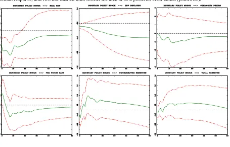
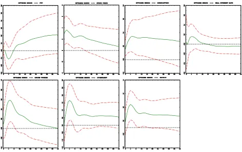
Figure 1: The baseline specification in ACRR (2016). The data span is 1965:01–2003:12. Green line denotes the
[image:16.595.76.531.480.772.2]16
As a result they identified the structural shock connected with this equation as the monetary policy shock. Figure 1 presents IRF’s to this shock.7 Although our approaches slightly differ along many dimensions we roughly got the same picture as in ACRR (2016).8 The most important difference is related to IRF of real GDP. In our case the negative response of real GDP to the contractionary monetary policy shock is obtained with more confidence. In addition, according to our median results, the maximum response suggests lowering real GDP by about 0.35 percent, whereas ACRR (2016) estimated this effect as 0.2 percent. Moreover the liquidity effect in nonborrowed reserves is better manifested than in ACRR (2016). Lastly it seems that all our 68% error bands are a little bit wider than those given in ACRR (2016).
In the development of their arguments ACRR (2016) put much emphasize on probabilities of negative coefficients of real GDP and GDP deflator in monetary policy equation. As demonstrated empirically by ACRR (2016), what drives their result concerning the IRF shape of real GDP is the restriction a0,11 ≤ 0 (coefficient of
real GDP is nonnegative). Below we explain theoretically the underlying statistics. In the baseline specification of ACRR (2016) we have
1
1 1
0 0 0 0 1 0 0
0 0 0 0 0 0 1
Z
L q−
′ =
(8)
1
1 1
1 0 0 0 0 0 0
0 1 0 0 0 0 0
0
0 0 0 1 0 0
S
L q−
−
′
− ≥
(9)
Note that by our proposition from appendix 3, the set of q1’s that fulfills (8)-(9) is
nonempty. Let us denote the i−th element of q1 as qi1. The instantaneous response
of real GDP to monetary policy shock is given by the (1,1) element of 1 0
A− =LQ i.e.
11 11
l q . Since l11 is strictly positive, this response will be negative iff q11<0. So the
whole problem amounts to introducing sign restriction that induces q11 <0 but
avoids the explicit assumption that instantaneous response of real GDP to monetary policy shock is negative (which would violate the Uhlig’s imperative to be agnostic
7 We used Uhlig’s monthly data set available at https://estima.com/procs_perl/uhligjme2005.zip.
All variables in logs but the federal funds rate. The data we used to produce Figure 1 span 1965:01– 2003:12. All computations in the paper are on the basis of 10.000 draws from the posterior. For monthly data we always set the number of lags in SVAR to 12.
8 We used slightly different prior (we are agnostic over the IRF’s, whereas ACRR (2016) chose to
17
along this dimension). Now, zero restrictions (8) imply that the last two elements in
1
q are zeros i.e. q51 =q61 = 0. Let
ij
l denote the ( , )i j element of L−1. Clearly
1
0
ii ii
l =l− > . Taking all considerations into account the first inequality in (9) reads as
1 21 31 41
11 11 21 31 41 0
l q− l q l q l q
− − − − ≥ and the second one as 1 32 42
22 21 31 41 0
l q− l q l q
− − − ≥ .9
The very reason why baseline identification in ACRR (2016) works is that diagonal elements ii
l dominate the remaining ones in the corresponding column of L−1. The
median estimates (together with 68% credible interval) of the first two sign restrictions in (9) are
11 21 31 41
(2.25,2.44)2.35 q (0.49,0.76)0.62 q ( 0.06,0.22)−0.08 q (0.08,0.36)0.22 q 0
− + + + ≥
21 31 41
(6.31,6.84)6.58 q (0.68,1.44)1.06 q ( 0.11,0.65)−0.27 q 0
− + + ≥
Clearly the second inequality highly favors negative or very small positive q21’s. This
reinforces the requirement that q11 should be negative to fulfill the first inequality. In
particular 90% of q21’s consistent with sign restrictions are contained in the interval
( 0.8, 0.04)− . This in turn implies that 90% of q11’s consistent with the first sign
restriction belong to the interval ( 0.89, 0.05)− − . As a result q11<0 holds with high
probability.
Anyhow, we asked ourselves the question whether the negative response of GDP to the contractionary monetary policy shock could be obtained 1) without explicit sign restrictions for this IRF (as in Uhlig (2005)), 2) avoiding clever restrictions on monetary policy equation proposed by ACRR (2016), 3) without standard (and commonly criticized) restriction that monetary policy shock could not influence GDP and prices on impact. Using the whole data set from Uhlig (2005) (up to and including the year 2003) we could not produce such a response. But with data ending in the mid 90’s, this was quite easy. In fact when Uhlig (2005) applied standard Choleski decomposition to the data up to year 2003 he obtained “price puzzle”, which he commented as “It may well be that the additional decade of data since 1992 has made this route [ i.e. introducing commodity prices] to resolving the price puzzle more difficult”. Since the data set was prepared for the problem from the perspective of mid 90’s we think that it is fair to play with the data constrained by that time. The clue how it may be accomplished was given by Uhlig (2005), since he wrote that “the identification of additional shocks can help in principle, as orthogonality between the shocks provides an additional restriction for identifying the monetary policy shock”. Hence in
9 Although the last sign restriction does not play any role in our reasoning it is very easy to see
18
addition to monetary policy shock we thought seriously about minimal zero restrictions for additional three shocks. Two of them may be identified as production shocks and the last one the information shock. Table 2 presents zero restrictions used by us.10 The entries in the Table 2 may be read as elements of the contemporaneous matrix A0.
Table 2: Zero restrictions imposed on A0
t
y pt pc t, rt nbrt trt
Prod X X X 0 0 0
Prod X X X 0 0 0
Inf X X X X 0 0
MP X X X X 0 0
Fin X X X X X X
Fin X X X X X X
“X” denotes unrestricted elements in A0 and “0” those restricted to zero. The first
column contains the reference names for the equation in SVAR. “Prod” refers to production sector, “Inf” refers to informational equation and “MP” is the monetary policy equation (“Fin” refers to financial sector but these equations play no role in our analysis). The main assumption underlying Table 2 is that nonpolicy variables do not respond contemporaneously to the policy variables (though instantaneous responses of these variables to the monetary policy shock are not restricted to zero). Clearly what makes the difference is the (3, 4) element in A0 i.e. unrestricted
coefficient in the informational equation of the federal funds rate. The rationale for this is that commodity price world market should respond immediately to the main indicators of monetary policy in a very large economy like the US. In addition to zeros induced by Table 2, we imposed Uhlig’s sign restrictions but confined only to the instantaneous response 1
0 A0−
Ψ = . Specifically, responses of GDP deflator, commodity price index, nonborrowed reserves are nonpositive, and those of federal funds rate nonnegative on impact. Hence we substantially weakened sign restrictions used by Uhlig (2005), who imposed them for horizons from 0 to 5 months. Using dataset spanning 1965:01–1995:12 we obtained IRF’s to the monetary policy shock identified by zero restrictions summarized in Table 2 and the sign restrictions confined to the impact responses, that are shown in Figure 2.
19
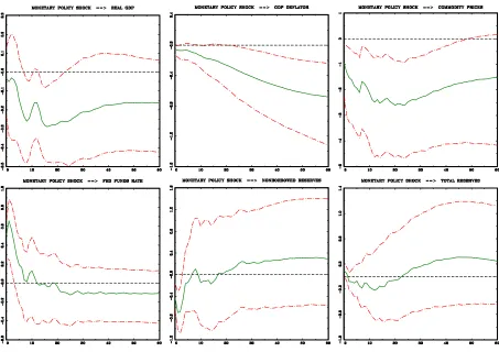
Figure 2: Monetary policy shock identified by zero restrictions summarized in Table 2 and the sign restrictions
confined to the impact responses. The data span is 1965:01–1995:12. Green line denotes the median response, and two dot-dashed lines restrict the area of 68% posterior error bands (pointwise).
Now we do not observe the output puzzle. The one standard deviation monetary policy shock leads to the significant decrease in the real GDP by about 0,3% after 7 months (and up to two years). Overall all the remaining plots look more reasonable in comparison with those presented in Figure 1. Both GDP deflator and commodity price index respond negatively in a significant way in all horizons. Responses of federal funds rate are sharper. As a consequence, the liquidity effect in responses of nonborrowed reserves is more revealed.
Following ACRR (2016), to gain some intuition we present the median estimates of the monetary policy equation (7) normalized on rt and using our zero and sign
restrictions (68% credible interval in parentheses)
, ,1
( 0.41,0.65)0.14 (0.008,2.72)0.81 (0.01,0.15)0.05
t t t c t t
r y p p lags ε
−
= + + + + (10)
20
that the assumed restrictions favor models that have moderate positive coefficients of the real GDP. If this is the case then the non-negligible negative support of the underlying marginal posterior for the coefficient of the real GDP may be accepted.
On the other hand the monetary policy rule estimated using baseline identification in ACRR (2016) (based on dataset truncated at 1995:12) looks as follows
, ,1
(0.32,4.62)1.20 (0.71,10.75)2.92 ( 0.45,0.23)0.06
t t t c t t
r y p p lags ε
−
= + − + + (11)
Since we explicitly imposed sign restrictions on coefficients of yt and pt, the
corresponding credible intervals cover only positive values. It is clear that baseline identification in ACRR (2016) implies that the set of possible monetary policy equations includes those highly responsive to the present state of the economy, see in particular the large upper bound in 68% credible interval for coefficient of the GDP deflator. Although ACRR (2016) addressed this point carefully, it still may be the case that the set of monetary policy rules consistent with the baseline restrictions in ACRR (2016) contain some implausible models of monetary policy behavior. In addition, the median estimate of the coefficient of commodity prices is negative and 68% credible interval contains both negative and positive values. Since the equation was estimated using the sample 1965:01–1995:12, to some extent this undermines the well thought and successful route to include commodity prices in the monetary policy function in order to avoid the price puzzle as advocated by Sims (1992) (see also Christiano et al. (1999)). Hence even if inclusion of commodity prices was found essential in the literature from 90’s (using the same dataset), the sign restrictions proposed by ACRR (2016) suggest something different. Finally we note that although our IRF’s presented in Figure 2 are quite different to those presented in Figure 1 (so as the estimated feedback rules), the FEVD’s in two models are remarkably similar.11
IX. OPTIMISM SHOCKS
Beaudry et al. (2014) used zero and sign restrictions to identify so-called optimism shocks. They applied Mountford and Uhlig’s (2009) penalty function approach (PFA) and obtain quite sharp results in terms of IRF’s and FEVD’s, which were criticized by ARRW (2016). For example, the latter authors, using their methodology, claim that contribution of optimism shocks to FEVD’s of many variables for whatever horizon was highly overestimated by Beaudry et al. (2014). We decided to check the robustness of these results with respect to our methodology.
21
The benchmark model of Beaudry et al. (2014) contains seven variables: Total Factor Productivity (TFP), stock price index, consumption, the real interest rate, hours worked, investment and output. The variables were logged (but the real interest rate) and taken in levels. For obvious reasons we use the same dataset and adopt the same model specification (i.e. four lags) as in Beaudry et al. (2014).12 They considered three basic identification schemes. All of them amounted to putting one zero and several sign restrictions, but were confined to the first column of 1
0 A0
−
Ψ =
only. They called them identification I, II and III. In all these identifications the optimism shock was assumed to have zero impact on TFP (in horizon “0”). In addition, in identification I, stock prices rise in response to optimism shock on impact, in identification II: stock prices and consumption rise in response to optimism shock on impact, and in identification III: stock prices, consumption and real interest rate increase in response to optimism shock on impact.
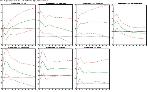
Main findings in Beaudry et al. (2014), who applied the PFA, were that optimism shock is crucial for business fluctuations since it leads to significant rise in consumption, hours worked, investment and output and results in the large corresponding FEVD’s. In fact, looking at Figure 1 in Beaudry et al. (2014) one may have impression that even identification I does a good job. Hence using only one zero and one sign restriction on impact, one may find that optimism shock is essential driver of the business fluctuations.
Figures 3, 4, 5 present IRF’s to optimism shock adopting identification I, II and III, respectively, using our algorithms. They are strikingly different in terms of IRF’s uncertainty to those showed in Beaudry et al. (2014). Hence we confirm the conclusion in ARRW (2016), who claimed that IRF’s bands presented in Beaudry et al. (2014) were artificially narrow and blamed the PFA for this. In particular, in contrast to Beaudry et al. (2014), identification I does not prove to be successful in obtaining sharp (i.e. statistically significant) results.
12 The author is extremely grateful to Jian Wang for making available the dataset used in Beaudry
22
Figure 3: Identification I. Green line denotes the median response, and two dot-dashed lines restrict the area of
68% posterior error bands (pointwise).
Figure 4: Identification II. Green line denotes the median response, and two dot-dashed lines restrict the area of
[image:23.595.71.543.417.715.2]23
Figure 5: Identification III. Green line denotes the median response, and two dot-dashed lines restrict the area of
68% posterior error bands (pointwise).
[image:24.595.69.536.485.719.2]Table 3 contains median estimates of FEVD due to optimism shock (together with 68% credible intervals) using our algorithms.
Table 3: FEVD’s due to optimism shocks for 4 and 40 quarters. Our methodology. Values in brackets show 68%
posterior credible interval.
Identification I Identification II Identification III
h = 4 qtrs. h = 40 qtrs. h = 4 qtrs. h = 40 qtrs. h = 4 qtrs. h = 40 qtrs.
TFP 0.02
[0.004, 0.05] 0.07 [0.02, 0.2] 0.02 [0.005, 0.05] 0.08 [0.02, 0.23] 0.02 [0.005, 0.06] 0.08 [0.02, 0.23]
stock prices 0.1 [0.02, 0.34] 0.09 [0.03, 0.25] 0.14 [0.03, 0.4] 0.12 [0.04, 0.28] 0.15 [0.03, 041] 0.13 [0.04, 0.31]
consumption 0.09 [0.01, 0.34] 0.1 [0.02, 032] 0.15 [0.03, 0.42] 0.12 [0.03, 0.36] 0.12 [0.02, 0.38] 0.15 [0.3, 0.39]
interest rate 0.1 [0.03, 0.3] 0.13 [0.05, 0.26] 0.1 [0.03, 0.3] 0.12 [0.05, 0.25] 0.12 [0.03, 0.33] 0.14 [0.06, 0.28]
hours worked 0.1 [0.02, 0.33] 0.11 [0.04, 0.26] 0.13 [0.03, 0.4] 0.13 [0.04, 0.29] 0.13 [0.03, 0.41] 0.12 [0.04, 0.29]
investment 0.1 [0.03, 0.29] 0.12 [0.04, 0.27] 0.13 [0.04, 0.35] 0.15 [0.06, 0.33] 0.12 [0.04, 0.35] 0.16 [0.06, 0.33]
output 0.09
[0.02, 0.31] 0.11 [0.03, 0.28] 0.15 [0.03, 0.39] 0.15 [0.05, 0.35] 0.13 [0.03, 0.37] 0.16 [0.05, 0.37]
24
TFP). One may say that each FEVD is about 1/ 7 ≈ 0.14. We interpret this as a
complete lack of identification. Further identifying (zero and/or sign) restrictions are probably needed to obtain economically significant results. On the other hand, the FEVD’s presented in Table 2 in Beaudry et al. (2014) point to substantially different results. There are many drastic discrepancies between our estimates. For example, using identification II, median estimates of FEVD of consumption and hours worked (for 4 quarters) are 0.74 and 0.46, respectively. Further, using identification III, Beaudry et al. (2014) presented median estimates of consumption and output (for 40 quarters), which were both equal to 0.52. Needless to say, in all these cases (and many other ones not mentioned) FEVD’s median estimates in Beaudry et al. (2014) are outside the 68% credible intervals given in our Table 3.
X. CONCLUSIONS
The paper presents new algorithms to deal with set identified SVAR models under zero and/or sign restrictions. Our methodology is similar to that presented in ARRW (2016), however we differ in some details. Paying special attention to many popular patterns of zero restrictions, we managed to simplify algorithms to draw from the posterior. We applied our methodology to challenge the output puzzle found in Uhlig (2005). Staying a priori agnostic about responses of output to monetary policy shock, we showed that it is not necessary to adopt sign restrictions on the systematic monetary policy equation proposed by ACRR (2016) to obtain significant real output drop as a result of contractionary monetary policy shock. In the second exercise, we largely confirm conclusions from ARRW (2016) concerning the results in Beaudry et al. (2014). Specifically the uncertainty in IRF’s given by Beaudry et al. (2014) is highly underestimated, and the estimates of FEVD’s presented in Beaudry et al. (2014) should be divided by two, three or even four to be consistent with ours.
25
APPENDICES
Appendix 1 (proof of Proposition 1):
Our goal is to evaluate
I , ( , ) 0; 1,...,
k k k i i
k Q Q′ = Z f ΠL q= =i k n< dQ
∫
. Consider the transformation1
( , )
i i
i i i i i
Z f L
Q q x G α β −
Π
′ = ′
, for each i=1,...,k (A1)
where αi : (zi×1), βi : (i− ×1) 1, xi : (n− − + ×zi i 1) 1 are “new” variables. Note that
in case i =1, β1 is empty. Further, Qi−1 =[q1…qi−1], with the convention that Q0 is
empty and Gi :n× − − +(n zi i 1) is any fixed (full column rank) matrix such that
1
I i
i i n z i
G G′ = − − + and
1 ( , ) 0 i i i
Z f L
G
Q−
Π ′ =
. The transformation (A1) serves its purpose as
long as ( ( , )f′ Π L Z Qi′⋮ i−1⋮Gi)′ is nonsingular for each i=1,...,k, which holds iff
1
( ( , )f′ Π L Z Qi′⋮ i− )′ has full row rank.
We need the Jacobian underlying the transformation (A1). Due to recursiveness of the transformation one has
1
( k i, , ;i i 1, , ) k ( i i, , )i i
i
J Q →α β x i = … k =
∏
=J q →α β x , so that1 2
1
1 1
( , ) ( , )
( k i, , ;i i 1, , ) ki i i
i i
Z f L Z f L
J Q α β x i k Q Q
−
= − −
′ Π Π
→ = = ′ ′ =
∏
… 1 2 1 11| ( , )(I ) ( , ) |
k
i n i i i
i Z f L Q Q f L Z
− − −
= ′ ′ ′
=
∏
Π − Π (A2)Implicit assumption in Jacobian derivation is that we always choose Gi such that the
determinant of ( ( , )f′ Π L Z Qi′⋮ i−1⋮Gi)′ is positive.
Of course Qk will be