An alternative probabilistic frontier analysis to the measurement of eco efficiency

(1)

Munich Personal RePEc Archive

An alternative probabilistic frontier

analysis to the measurement of

eco-efficiency

Kounetas, Konstantinos and Polemis, Michael and Tzeremes,

Nickolaos

University of Patras, University of Piraeus, University of Thessaly

5 May 2019

Online at

https://mpra.ub.uni-muenchen.de/93686/

(2)

An alternative probabilistic frontier analysis to the measurement of eco-efficiency

Konstantinos Kounetasa_{, Michael L. Polemis}b,c*_{, Nickolaos G. Tzeremes}d

a

Department of Economics, University of Patras, Rio 26504, Patras, Greece

b_{Department of Economics, University of Piraeus, Piraeus, Greece , Email:}

[email protected] (*corresponding author) c _{Hellenic Competition Commission, Athens, Greece}

d_{Department of Economics, University of Thessaly, Greece.}

Abstract

This study applies a nonparametric time dependent conditional frontier model to estimate and evaluate the convergence in eco-efficiency of a group of 51 US states over the period 1990-2017. Specifically, we utilize a mixture of global and local pollutants (carbon dioxide CO2, sulphur dioxide SO2 and nitrogen oxides NOx) to capture the environmental damage caused by the anthropogenic activities. The empirical findings indicate divergence for the whole sample, while specific groups of convergence club regions are formulated dividing the US states into worst and best performers. Moreover, Our findings reveal significant convergence patterns between the US regions over the sample period.

Keywords: Eco-efficiency; Convergence clubs; Order-m estimators; Non parametric frontier analysis; US regions

(3)

1. Introduction

Despite the primary contribution of the French physicist and philosopher

Jean-Baptiste Joseph Fourier, The analytical Theory of Heat, who was the first to describe

back in 1822 the greenhouse effect and the underlying theoretical mechanisms of

climate change, the scientific community has recently acknowledged that

environmental damage triggered by anthropogenic activities is a global challenge that

incurs a global response.1

As a result, Kyoto Protocol was adopted in December 1997, setting legally

binding targets to mitigate greenhouse gas emissions for the period 2008-2012. To

achieve these objectives, three flexible instruments were created (i.e., emissions

trading, joint implementation and clean development mechanism) giving the

opportunity to ratified countries to use the market mechanism. This global awareness

covers also the post Kyoto period and a new international agreement is in force from

December 2015 (Paris Agreement).2

One of the main aspects in achieving these goals is sustainable development and

eco-efficiency. Kuosmanen and Kortelainen (2005) were the first who coined the term

“eco-efficiency” to describe the ability of an economy to produce the maximum level

of economic output (desirable output) while causing the minimum environmental

distortion (undesirable output).

In an influential study, Kuosmanen and Kortelainen, (2005) employ a Data

Envelopment Analysis (DEA) framework in order to measure eco-efficiency,

accounting for various substitution possibilities between different natural resources and

1_{Actually he was the first to argue that the Earth’s atmosphere acts to raise the planet’s temperature latter}

known as the “greenhouse” effect (Fourier, 1878)

2_{Paris Agreement, aims to strengthen the ability of countries to deal with the impacts of climate change}

(4)

emissions. However, this analysis is developed in a static setting since it does not

account for technical change or explain changes in environmental performance over

time (Kortelainen, 2008). In order to deal with this limitation, Kortelainen (2008),

builds a general framework to account for dynamic environmental performance

analysis. Specifically, this study, constructs an environmental performance index (EPI)

by applying frontier efficiency techniques combined with a Malmquist index approach.

The sample used in this work includes 20 European Union (EU) member states over

the period 1990–2003. The empirical findings indicate that improvement in overall

environmental performance can mostly be attributed to environmental technical

change, while relative eco-efficiency change has minor contribution for most of the

sample countries.

In another study, Halkos et al, (2013) apply an additive two-stage DEA model

along the lines of Chen et al., (2009) to create a sustainability composite index

consisting of production efficiency and eco-efficiency. Specifically, they employ a

window-based approach on a sample of 20 countries over the time period 1990–2011.

The empirical findings justify inequalities among the sample countries over the two

distinct stages. Specifically, they argue that eco-efficiency stage is characterized by

large inequalities among the sample countries and significantly lower efficiency scores

than the overall sustainability efficiency and the production efficiency. Moreover, the

authors suggest that a country’s high production efficiency level is not related to a high

eco-efficiency performance.

During the last years, several researchers have attempted to investigate

convergence patterns in eco-efficiency in greenhouse gas emissions. The study of

Camarero et al, (2013a) employ DEA techniques and directional distance functions to

(5)

countries following Phillips and Sul (2007) methodology. The empirical results indicate

the existence of four convergence groups among the EU-periphery. In a similar vein,

Camarero et al, (2013b) examine convergence patterns in eco-efficiency scores drawn

from a sample of 22 OECD countries over the period 1980–2008 taking also into

account three “undesirable” outputs (CO2, NOX and SOX emissions). The authors argue

that in general terms, eco-efficiency indicator has been increased over the sample

period, indicating environmental performance. Moreover, some convergence groups

are formed consisting of various sample countries based on their eco-efficiency

performance. Specifically, Switzerland can be characterized as the most eco-efficient

country, followed by some Scandinavian countries (i.e, Sweden, Iceland, Norway and

Denmark). On the other hand, some Southern EU member states (e.g., Portugal, Spain

and Greece) followed by Canada and the United States, are among the worst

performers.

This study contributes the literature in many fronts. First and foremost, we apply

one of the most innovative Data Envelopment Analysis (DEA) methods (i.e., time

dependent conditional frontier model) to estimate the eco-efficiency indicator drawn

from a separable production function of the electricity sector. Specifically, we use a

flexible nonparametric partial frontier analysis to estimate in the first stage the

eco-efficiency scores per US region (states). Second, in the applying methodological

framework we take into account time effects and the effects generated by environmental

degradation without imposing any restrictive assumptions on the statistical models

describing the data generating process (Simar and Wilson, 2011; Daraio et al., 2018).

The third novelty of this study lies on its application of the proposed model. To our

knowledge there are few studies for EU member states or OECD countries estimating

(6)

relationship for the 51 US states. Fourth, we deliver for the first time in the literature a

convex Order-m eco-efficiency measure, which is analogous to the original DEA based

eco-efficiency indicator developed by Kuosmanen and Kortelainen (2005) but more

robust to extreme values and potential outliers. We then use this indicator to test for the

robustness of our findings. Lastly, we move beyond the well-known convergence

methodology of Phillips and Sul (2007; 2009) by employing distributional dynamics

organized along a Markov chain. In this way, we use stochastic kernels to describe both

the change in the external shape and the intra-distribution dynamics of the

cross-sectional distribution in order to trace possible convergence clubs (Kounetas and

Zervopoulos, 2019).

The remainder of the paper is structured as follows. Section 2 presents the data

and the methodology applied. Section 3 discusses the empirical findings concerning the

estimation of eco-efficiency scores on each US region over the sample period

(1990-2017), and the formulation of convergence clubs. In Section 4 the necessary robustness

checks are presented by comparing our main results with two alternative eco-efficiency

measures (e.g., conventional DEA based indicator and convexified order-m estimator).

Lastly, Section 5 encapsulates the main findings of the paper.

2. Data and Methodology

This section describes the data used in the empirical analysis, while providing

the summary statistics for all the sample variables. Moreover, we discuss and analyze

the probabilistic frontier analysis along with the convergence methodology applied (see

Phillips and Sul, 2007; 2009) that we used to empirically estimate and test for the

(7)

2.1 Data description

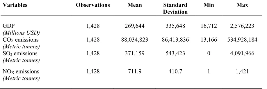
Our empirical analysis is based on a panel dataset of 1,428 annual observations,

spanning the period 1990-2017 (N = 51 and T = 28). The selected sample includes all

the 51 US states. The starting date for the study was strictly dictated by data availability,

while the final date observation, represents the last year for which data mostly regarding

the US Energy Information Administration (EIA) were available at the time the

research was conducted.

The level of economic growth is proxied by per capita real GDP across US

states, measured in millions of 2009 USD. 3_{The latter is drawn from the Regional}

Economic Accounts of the Bureau of Economic Analysis (BEA) and provides the

market value of goods and services produced by the labor and property located in a US

state.4 _{This variable can be regarded as an inflation-adjusted measure that is based on}

national prices for the goods and services produced within each region (US state).

The environmental variables used in the estimation of the eco-efficiency

indicator, refer mainly to global and local pollutants such as CO2, SO2 and NOx

emissions. The latter are measured in metric tons for the 51 US states generated by

power plants from all energy sources (i.e., coal, petroleum, geothermal, natural gas,

wood and wood derived fuels, other biomass, other gases, and other emissions such as

CO2 emissions from municipal solid waste) over the period 1990-2017. The reason for

using the CO2 emissions as the only global pollutant stems from the fact that it

constitutes the main contributor to global warming and therefore environmental

3

Similarly, to Camarero et al, (2013a), we moved the base year to the beginning of the period to avoid bias in favour of convergence around the GDP base year. The results did not exhibit significant differences and are available upon request.

4

(8)

regulations aimed at reducing CO2 emissions have been in force the longest and in most

cases are the most restrictive (Camarero et al, 2013b).

To get a clear picture of the environmental degradation in the US, we include in

our analysis all the different types of power plants consisting of commercial (non)

co-generators, industrial (non) co-co-generators, electric utilities, etc. The relevant variables

were drawn from the EIA.5_{The following table, portrays the descriptive statistics for}

all the variables used in the empirical analysis.

<Insert Table 1 about here>

2.2 Probabilistic frontier analysis

According to Kuosmanen (2005) eco-efficiency is referred to the production of

economic output with minimal environmental degradation. Based on the work by

Koopmans (1951), Kuosmanen and Kortelainen (2005) provide an eco-efficiency

measure using data envelopment analysis (DEA) estimators. They have characterized

the pollution-generating technology set as:

Φ = , ∈ ℝ value added can be generated with damage . (1)

Equation (1) implies all technical feasible combinations of states’ value added

levels and environmental damage = ! , … , #. Then using the Farrell (1957)

measure, we can present state’s eco-efficiency level as:

$ , = inf&$| $ , ∈ Φ(. (2)

Following the framework by Daraio and Simar (2007b) an observed state ₎, ₎

defines an individual possibilities set as:

5

(9)

* ), ) = , ∈ ℝ ≥ ), ≤ ) . (3)

The union of these sets (equation 3) provides us a Free Disposal Hull-FDH (Deprins et

al. 1984) type of eco-efficiency estimator as:

Φ./01 = ⋃ *6)7 ), ) = , ∈ ℝ ≥ ), ≤ ), 3 = 1, … , 5 . (4)

Then the DEA-type of eco-efficiency measure is obtained by the convex hull

(CH) of Φ._/01 as:

Φ.089 = :; ⋃ *6)7 ), ) = , ∈ ℝ ≤ ∑ =6)7 ) ); ≥ ∑ =6)7 ) ),

for = , … , =6 @. A. ∑ =6)7 ) = 1; =) ≥ 0, 3 = 1, … , 5 . (5)

Based on the probabilistic framework by Cazals et al. (2002) and Daraio and Simar

(2005) the pollution generated technology can be also characterized by the joint

probability measure C, D as :

Β0F , = Prob C ≤ |D ≥ Prob D ≥ = H0|F | IF . (6)

Then the probabilistic version of the eco-efficiency measure can be defined as:

$ , = inf J$| KH0|F $ | L > 0N = inf&$|Β0F $ , > 0(, (7)

where OP_0|F,6 | =∑WRXY_∑Q 0_{Q ,F}RST,FRUV RUV W

RXY .

According to Daraio and Simar (2007b) the eco-efficiency, which are based on

the FDH and the DEA estimators, are very sensitive to extreme values and outliers. In

order to avoid such shortcomings according to Cazals et al. (2002) it is more appropriate

to apply the Order-m estimators in order to construct the eco-efficiency measures.

Previously H_0|F ⋅| defines state’s environmental pollutants (damage) C at the value

(10)

this support in order to define state’s eco-efficiency levels, it uses the average of the

minimal value of environmental pollutants (damage) for [ states which are randomly

drawn according to H_0|F ⋅| . As a result in order to evaluate state’s eco-efficiency

levels it uses as a benchmark only the states producing at least the value added level .

According to Daraio and Simar (2007b) for a given value added level, we consider [

i.i.d. random variables C , … , C_\ generated by the conditional p-variate distribution

function H_0|F ⋅| obtain a random production set as:

Φ]\ = , ́ ∈ ℝ ≥ C), ́ ≥ , 3 = 1, … , [ . (8)

Therefore, the Order-m eco-efficiency measure can be defined as:

$\ , = _0|F $̃\ , |D ≥ , (9)

where $̃_\ , = inf $| $ , ∈ Φ]_\ and __0|F is the expectation in relation to

H0|F ⋅| . As a result the Order-m eco-efficiency measure is the expectation of the

environmental damage efficiency score of the state , when is compared with the

[ states randomly drawn with replacement from the population of states producing at

least the value added level . Moreover, the estimated Order-m frontier is the set

of! _\a , # ∈ Φ, where _\a is the radial projection of , ∈ Φ on the Order-m

frontier in the environmental damage direction.

We can calculate the Order-m eco-efficiency measure as:

$̂\ , = _P0|F $̃\ , |D ≥ = c K1 − HP0|F e | L \

e

f

g . (10)

Finally, we can obtain a convex Order-m eco-efficiency estimator as:

$̂\h , = inf $| ≤ ∑ =6)7 ) ); $ ≥ ∑ =6)7 ) i\,)a , for = , … , =6 @. A. ∑ =6)7 ) =

(11)

According to Daraio and Simar (2007b) it holds:

$ , ≤ $\h , ≤ $\ , , (12)

where $ , is the Kuosmanen, and Kortelainen’s (2005) eco-efficiency measure;

$\h , is the global convex Order-m based efficiency measure. The

eco-efficiency and the convex Order-m measure can take values from zero to one

(eco-efficient region). Finally $_\ , is an Order-m based eco-efficiency measure. It is

worth mentioning that the efficiency scores can take values greater than one (indicating

a super eco-efficient region). Lastly, as suggested by Cazals et al. (2002) partial

frontiers such as Order-m estimators are less sensitive to outliers.

2.3 Convergence methodology

Phillips and Sul (2007), propose an econometric approach for testing the

convergence hypothesis and the identification of convergence clubs. Their method uses

a nonlinear time-varying factor model and provides the framework for modelling

transitional dynamics as well as long-run behavior (Apergis et al, 2013). The

methodology applied can be outlined as follows:

If X_it is the solely factor of a panel data set (X denotes the rating for a given

journal,i denotes the journal list and t the time), then

,

t it it

X =δ µ (13)

where δ_it measures the deviation of journal list’s i ranking from the common trend µ_t

and can be represented as:

, )

( 1 a

it i i

it =δ +σ ξ L t − t−

(12)

where δ_iis fixed, ξ_itis weakly dependent over twith ξ_it ~iid(0,1) and L(t) is a slowly

varying function with L(t)→∞when t→∞. The null hypothesis of convergence for

all i (H₀) versus the alternative of non-convergence for some i (H_A) can be expressed

as:

δ δ_i =

H₀: and a≥0; H_A:δ_i ≠δ or a<0. (15)

The null hypothesis in (15) can be tested through the following regression:

, ˆ log ˆ ˆ ) ( log 2

log 1 _t

t u t b c t L H H + + = −       (16)

for t=[rT],[rT]+1,...,Twith some r>0.6_{In (4),}

∑

= −

= N

i it

t N h

H 1 2 ) 1 ( ) / 1 (

∑

= − = − = = N i it it N i it it it N X N X h 1 1 1 1 _δ δ

, L(t)=log(t+1)and bˆ=2aˆ where aˆis the

least-squares estimate of a inH₀ (null hypothesis).

Based on the above analysis, Phillips and Sul (2007) argue that the hypothesis

of convergence can be tested through a one-sided t-test. Specifically, the alternative

hypothesis of non-convergence cannot be rejected at the 5% level if t_bˆ <−1.65.

Finally, we apply Phillips and Sul (2009) procedure to determine the existence of

further convergence clubs.

3. Results and discussion

This section presents the empirical findings of the study. In the first stage, we

present the results of the eco-efficiency scores of 51 US regions constructed by applying

the probabilistic frontier analysis (order-m estimator) and compare these estimates with

(13)

the results of similar studies reported by the existing literature. Then in the second stage,

we test for club formulation convergence between the sample regions utilizing the

Phillips and Sul (2007; 2009) methodology.7

3.1 Eco-efficiency scores

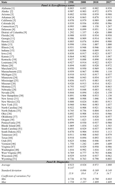
Table 2 presents the results of the regional eco-efficiency scores for selected

years derived from the applied probabilistic frontier analysis (i.e., order-m estimators).8

We must bear in mind that in contrast to other eco-efficiency indicators appeared in

similar studies (see for example Kuosmanen and Kortelainen, 2005; Picazo-Tadeo et

al. 2011; Camarero et al, 2013b) the proposed one can take values greater than one,

implying higher levels of eco-efficiency. It is worth mentioning that the empirical

findings have been obtained setting m = 20.9_{It must be stressed that contrary to the full}

frontiers the order-m efficiency scores denote the expectation of the minimal input

eco-efficiency score of a region, when compared to twenty other regions randomly drawn

with replacement from the population of regions having the same or higher GDP per

capita (Halkos and Tzeremes, 2013).

The eco-efficiency score results reveal that 3 out of 51 states (e.g., Vermont,

Rhode Island and District of Columbia) constitute the most eco-efficient regions since

their scores exceed unity for all the selected years (see Panel A). In other words, these

three states are the only regions across the US territory that remain above the efficient

boundary of the order-m frontier (“best” performing regions). As a result, they can be

characterised as eco-efficient since they use fewer pollutants levels (CO2, SO2 and

7_{For our empirical estimations, we used the STATA codes appeared in Du (2017).}

8_{To conserve space, we only report the eco-efficiency scores for the selected four years (1990, 2000,}

2010 and 2017). The detailed results for each sample year are available from the authors on request.

9_{To check for robustness, we have experimented with other values for m (m = 10, 15, 25, 30) but the}

(14)

NOx) compared only to states having the same or higher level of economic growth

(GDP per capita). On the other hand, the regions of West Virginia and Wyoming report

the lowest eco-efficiency scores ranging from 0.736 to 0.806 (“worst” performing

regions).

As it is evident, Wyoming is the region with the lowest eco-efficiency factor

equal to 0,8 for the latest available year (2017). This means that the specific region uses

20% more inputs in the production process than the expected value of the minimum

input level of m other regions (in our case 20) drawn from the population of regions

producing a level of output equal or greater than the efficient one (see Daraio and Simar,

2007b; Halkos and Tzeremes, 2013). On the other hand, the state of Vermont exhibits

the highest score compared to the rest US regions remaining well above the efficient

boundary of the order-m frontier taking the value of 1,609 in 2017.

In addition, the eco-efficiency score in four regions (California, District of

Columbia, Illinois and Indiana) equals to unity, implying that the specific entities are

on the efficient boundary of the order-m frontier. As a consequence, we argue that the

relevant regions appear to have the same levels of pollutants than the expected value of

the minimum level of pollutants of the twenty other regions (i.e., m = 20) drawn from

the total population of regions having at least the same level of economic growth.

Overall, the summary statistics reveal low disparities of regional eco-efficiency

scores among the US states since the standard deviation and the coefficient of variation

appear to be relatively low exhibiting a downward trend throughout the selected years

(see Panel B). Lastly, the average eco-efficiency indicator shows an upward trend over

the sample period (i.e., reaching 1,008 in 2017 compared to 0,923 in 1990).

(15)

3.2 Convergence clubs formulation

Having estimated the efficiency scores by applying the probabilistic frontier

analysis, we limit our attention to the existence of eco-efficiency convergence clubs

using the Phillips and Sul (2007) methodology.

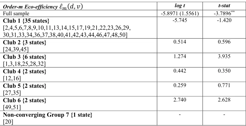
The results drawn from the convergence algorithm are illustrated in Table 3. As

it is evident, the null hypothesis of convergence cannot be accepted for the US as a

whole (full sample) since the t-statistic is smaller than the critical value (-1.65) at 5%

level of statistical significance. This means that we must test for the existence of

separate convergence clubs drawn from the whole sample (i.e., 51 regions).

It can be easily shown that there are six convergence clubs (see Column 1)

consisting of different number of regions. In particular Club 1 consists of 35 states

(Alaska, Arkansas, California, Colorado, Connecticut, Delaware, District of Columbia,

Florida, Georgia, Idaho, Illinois, Indiana, Kansas, Louisiana, Maryland, Massachusetts,

Michigan, Missouri, Nevada, New Hampshire, New Jersey, New York, North Carolina,

Oklahoma, Oregon, Rhode Island, South Carolina, South Dakota, Tennessee, Texas,

Vermont, Virginia, Washington and Wisconsin). Club 2 has 2 members (Minnesota,

Pennsylvania and Utah), while Club 3 consists of 6 regions (Alabama, Arizona,

Kentucky, Mississippi, Nebraska and New Mexico). Moreover, Club 4 and 5 have also

2 members (Hawaii and Iowa; Montana and North Dakota respectively). Finally, the

rest of the regions (i.e., West Virginia and Wyoming) do convergence formulating Club

6.

In these clubs, the estimated t-statistics are larger than -1.65, indicating

convergence (i.e., acceptance of null hypothesis). However, the state of Maine (20)

(16)

performing regions fall within the first Club (i.e., Vermont, Rhode Island and District

of Columbia). On the contrary, the “worst” performers (i.e., West Virginia and

Wyoming) do convergence formulating Club 6.

Having delineated the convergence clubs based on Phillips and Sul (2007)

generic algorithm, the analysis continues with the interpretation of the speed of

convergence among the formulated clusters. A deeper inspection of Table 3 uncovers

some important remarks.

First, the speed of convergence varies significantly across the six formulated

clubs.10_{Second, the first club, which includes among others the “}_best_{” performing}

regions, records an absolute value of α = 2,8 approximately, indicating a high

adjustment speed to convergence among other clubs. This finding runs contrary to the

study of Camarero et al, (2013b), in which convergence speed is slower in those clubs

consisting of higher eco-efficiency country scores, compared to other clubs with lower

efficiency scores. Apart from the different sample, this discrepancy might also be

attributed to the different methodology applied, since the study of Camarero et al,

(2013b) employs a full frontier analysis in which the variable of interest (i.e.,

eco-efficiency indicator) is bounded between zero and one, where one (zero) denotes the

most (least) eco-efficient country. Third, the “worst” performers (Club 6) are

characterized by a large value of convergence speed equal to α = _{1,37 approximately.}

This means that the two members of this club (West Virginia and Wyoming) are

approaching one another more rapidly in relative terms. This value is almost six times

greater than the relevant one (α = 0.235) appeared in Camarero et al, (2013b). Lastly,

10_{According to Phillips and Sul (2007), the speed of convergence α can be calculated as half the estimated}

(17)

slow convergence is found among the regions of Clubs 5, 4 and 2, whereas the members

of Clubs 1 and 6 are approaching more rapidly.

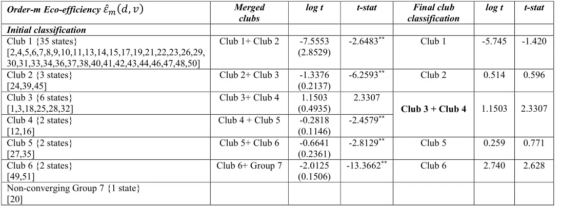
As a final step, we use the Phillips and Sul (2009) methodology to investigate

the existence of convergence merging clubs. The following table, presents the empirical

results drawn from the applied methodology. As it is evident, we accept the null

hypothesis of convergence only in one case (Club 3 and Club 4), since the relevant

t-stat (2.3307) is larger than its critical value (-1.65). This means that these two primary

clubs formulate one larger (merged) club with moderate convergence speed (α = 0.575).

On the contrary, none of the other existing primary clubs can be merged since the null

hypothesis of club-merging for all the combinations of two or three clubs is rejected

(t-stat>-1.65). In this case, the initially formed clubs as described above are the

appropriate ones. Therefore, after club-merging, there are five convergence clubs (i.e.

primary clubs 1,2,5, 6 and one merged Club 3+4).

4. Robustness checks

In this section, we perform the necessary robustness checks by using two

alternative eco-efficiency indicators namely the conventional eco-efficiency and the

robust eco-efficiency indicator.

Firstly we calculate the original eco-efficiency measure as proposed by

Kuosmanen and Kortelainen (2005) and formally presented in Equation (5). This

measure constitutes a DEA based indicator under the assumption of Variable Returns

to Scale (VRS). However, as any other DEA estimator is sensitive to potential extreme

(18)

theoretical framework by Cazals et al. (2002) we provide an Order-m based

eco-efficiency measure (see Equation 10). This indicator is more robust compared to the

original DEA based eco-efficiency indicator since it does not envelop all the data points

and therefore is more resistant to potential effects form outliers and extreme values.

However, this indicator is not convex as the DEA estimator, therefore, we convexify

the Order-m based eco-efficiency indicator to provide rigorous economic intuition. (see

Equation 11). 11

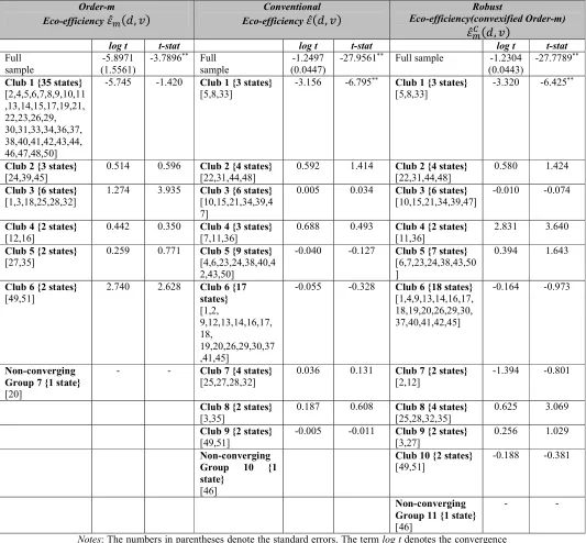
The results from the initial club clustering are displayed in Table 5. To get a full

picture of convergence patterns and club classifications among the sample regions, we

conserve the order-m estimator results. From the careful examination of the relevant

table some interesting results emerge. First, the null hypothesis of convergence does

not seem to hold for the whole sample regions since the t-statistic is smaller than the

critical value (-1.65) at least at 5% level of significance. Second, regarding conventional

eco-efficiency indicator, the Phillips and Sul (2007) algorithm revealed nine initial

convergence clubs and one non-converging group. Third, the robust eco-efficiency

scores provided similar convergence patterns (i.e., ten clubs and one non-converging

group). Finally, in line with the order-m eco-efficiency indicator, we exemplify that the

best (worst) performing regions fall within the first (last) convergence club

respectively. This implies that the empirical findings are rather robust.

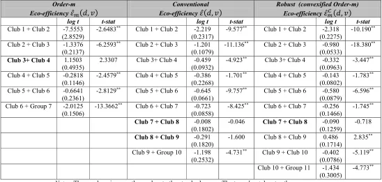
Having identified the existence of specific convergence clubs among the sample

regions, we turn our attention on whether it is possible to merge some of the initial

convergence clubs found above. Therefore, we apply the Phillips and Sul (2009)

11

(19)

methodology on the two different eco-efficiency measures (conventional and robust

eco-efficiency scores).

The relevant results are illustrated in Table 6. Regarding the conventional

eco-efficiency indicator, we fail to reject the null hypothesis of convergence in two cases

(Club 7+8 and Club 8+9). On the contrary, none of the other existing primary clubs can

be merged. Similar findings can be postulated by examining the robust eco-efficiency

indicator. In this case, only the initial convergence club 7 (Alaska and Hawaii) and club

8 (Mississippi, Nebraska, New Mexico and North Dakota) can be merged since the

relevant t-statistic (-0.718) falls within the null hypothesis region (i.e., larger than the

critical value of -1.65).

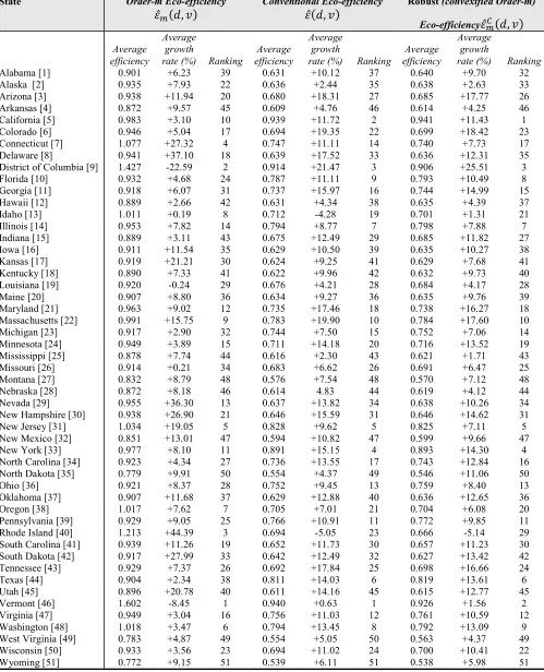
Finally, to draw sharp conclusions about the interpretation and the comparison

of the three alterative eco-efficiency indicators, we provide the average efficiency score

over time (1990–2017) for each region along with the average annual growth rate (%

percent change from 1990 to 2017).

As it is evident from the following table, the average annual growth rates do not

appear to have significant differences across the three eco-efficiency indicators

providing a stable convergence pattern. Regarding the magnitude, we argue that

eco-efficiency as it is measured by three different indicators (i.e., conventional, convexified

robust estimator and order-m estimator), portrays significant positive changes in most

of the sample regions (see for example Delaware, New Hampshire, South Dakota and

Connecticut and Arizona). Regarding order-m eco-efficiency scores, Rhode Island and

Delaware are the regions with the highest average annual growth rate (+44.39% and

+37.10% respectively), whereas District of Columbia achieves the lowest growth rate

(20)

scores since 1990. This might be attributed to various reasons mainly stemming from

the legislative and regulatory framework for environmental protection, which has been

greatly improved within the last twenty years, targeting, among others, global warming

and sustainable development (Halkos et al., 2015). As a result, the SO2 emissions in

Rhode Island have been significantly reduced reaching an annual growth rate of -95%

(from 3,282 in 1990 to 156 in 2017). Similarly, SO2 and NOx emissions have been

successfully mitigated in Delaware (99% and 94% respectively).

However, the positive average growth rates are much smaller when we measure

efficiency by the other two approximations (e.g., conventional and robust

eco-efficiency indicators). Regarding robust eco-eco-efficiency indicator, only six eco-efficiency

scores change more than 15% in average during the time period (District of Columbia

with 25.51%, Colorado with 18.42%, Arizona with 17.77%, Massachusetts with

17.60%, Tennessee with 16.66% and finally Maryland with 16,27%). We must mention

thought that the results do not dramatically change when we account for conventional

eco-efficiency indicator. In this case, we observe that there are ten regions with an

annual growth rate more than 15%.

It is worth emphasizing that most of the sample regions appear to have a similar

ranking pattern across the three indicators for the latest available sample year (2017).

From the careful inspection of the relevant table (see ranking column), one cannot fail

to observe that specific states such as Vermont (1st_{place in two indicators and 2}nd_place

in the third one), District of Columbia (2nd_{place in one indicator and 3}rd_{place in the}

other two) and New Jersey (5th_{place in all of the three indicators) belong to the highly}

ranked regions in all of the three different eco-efficiency measures. This means that the

relevant regions constitute the “best” performers in terms of their eco-efficiency

(21)

On the other hand, Wyoming, West Virginia, North Dakota, Montana and New

Mexico constitute the “worst” performing regions based on their low ranking positions

across the three different indicators. The above findings confirm the existence of the

previously discussed convergence clubs (clusters) across the US territory. However, for

some US states (see for instance Rhode Island, Connecticut and Oregon), the order-m

indicator reveals substantial differences compared with the rest two eco-efficiency

approximations.

(22)

5. Conclusions

The need of modern economies to produce with fewer impacts on the

environment and less consumption of natural resources constitutes a challenging issue

for the environmental economists and researchers worldwide. Despite the significant

contributions on this field, mostly made from the empirical standpoint, the existing

literature on this topic is still in its infancy. We attempt to shed light on this ongoing

research by applying a nonparametric time dependent conditional frontier model to

estimate and evaluate the convergence in eco-efficiency of a group of 51 US states over

the period 1990-2017. For this reason, we utilize a mixture of global and local pollutants

(carbon dioxide CO2, sulphur dioxide SO2 and nitrogen oxides NOx) to capture the

environmental damage caused by the anthropogenic activities.

The empirical findings indicate divergence for the whole sample, while specific

groups of convergence club regions are formulated dividing the US states into worst

and best performers. Our findings reveal significant convergence patterns between the

US regions over the sample period. Lastly, our results survive robustness checks under

the inclusion of two alternative measures of eco-efficiency (e.g. robust and

(23)

[image:23.612.80.539.130.284.2]

List of Tables

Table 1: Summary statistics

Variables Observations Mean Standard

Deviation

Min Max

GDP

(Millions USD)

1,428 269,644 335,648 16,712 2,576,223

CO2 emissions

(Metric tonnes)

1,428 88,034,823 86,413,836 13,166 534,928,184

SO2 emissions

(Metric tonnes)

1,428 371,159 543,423 0 4,091,966

NOX emissions

(Metric tonnes)

(24)

[image:24.612.118.491.88.686.2]

Table 2: Order-m Eco-efficiency scores $̂_\ , per selected year

State 1990 2000 2010 2017

Panel A: Eco-efficiency scores

Alabama [1] 0.883 0.892 0.902 0.938 Alaska [2] 0.907 0.903 0.972 0.979 Arizona [3] 0.882 0.930 0.939 0.988 Arkansas [4] 0.834 0.863 0.878 0.913 California [5] 0.970 0.979 0.989 1.000 Colorado [6] 0.939 0.936 0.950 0.986 Connecticut [7] 0.995 1.000 1.158 1.267 Delaware [8] 0.863 0.899 0.951 1.184 District of Columbia [9] 1.292 1.357 1.426 1.000 Florida [10] 0.908 0.935 0.934 0.950 Georgia [11] 0.906 0.909 0.914 0.961 Hawaii [12] 0.885 0.876 0.894 0.908 Idaho [13] 0.998 1.016 1.007 1.000 Illinois [14] 0.931 0.948 0.946 1.003 Indiana [15] 0.885 0.886 0.889 0.913

Iowa [16] 0.858 0.917 0.923 0.957

Kansas [17] 0.864 0.902 0.939 1.047 Kentucky [18] 0.857 0.888 0.890 0.920 Louisiana [19] 0.927 0.914 0.922 0.925 Maine [20] 0.894 0.883 0.920 0.972 Maryland [21] 0.950 0.950 0.969 1.036 Massachusetts [22] 0.959 0.967 0.998 1.110 Michigan [23] 0.910 0.915 0.917 0.937 Minnesota [24] 0.940 0.943 0.954 0.977 Mississippi [25] 0.856 0.871 0.883 0.922 Missouri [26] 0.920 0.913 0.914 0.921 Montana [27] 0.793 0.827 0.839 0.863 Nebraska [28] 0.853 0.848 0.883 0.922 Nevada [29] 0.844 0.894 1.024 1.150 New Hampshire [30] 0.891 0.908 0.933 1.130 New Jersey [31] 1.000 0.988 1.046 1.190 New Mexico [32] 0.808 0.824 0.881 0.913 New York [33] 0.960 0.964 0.983 1.037 North Carolina [34] 0.922 0.908 0.921 0.962 North Dakota [35] 0.745 0.756 0.804 0.819

Ohio [36] 0.892 0.908 0.918 0.966

Oklahoma [37] 0.857 0.919 0.920 0.957 Oregon [38] 0.976 1.023 1.018 1.050 Pennsylvania [39] 0.899 0.930 0.937 0.980 Rhode Island [40] 1.069 1.034 1.625 1.543 South Carolina [41] 0.893 0.929 0.937 0.993 South Dakota [42] 0.870 0.904 0.918 1.113 Tennessee [43] 0.911 0.908 0.945 0.979 Texas [44] 0.910 0.894 0.893 0.931

Utah [45] 0.825 0.866 0.946 0.997

Vermont [46] 1.758 1.242 1.699 1.609 Virginia [47] 0.957 0.929 0.950 0.986 Washington [48] 1.016 0.992 1.016 1.052 West Virginia [49] 0.769 0.777 0.793 0.806 Wisconsin [50] 0.929 0.919 0.937 0.962 Wyoming [51] 0.736 0.763 0.790 0.803

Panel B: Diagnostics

(25)

[image:25.612.101.511.86.297.2]

Table 3: Primary club convergence results

Order-m Eco-efficiency $̂_\ , log t t-stat

Full sample -5.8971 (1.5561) -3.7896**

Club 1 {35 states}

[2,4,5,6,7,8,9,10,11,13,14,15,17,19,21,22,23,26,29, 30,31,33,34,36,37,38,40,41,42,43,44,46,47,48,50]

-5.745 -1.420

[24,39,45]

0.514 0.596

[1,3,18,25,28,32]

1.274 3.935

[12,16]

0.442 0.350

[27,35]

0.259 0.771

[49,51]

2.740 2.628

Non-converging Group 7 {1 state}

[20]

- -

Notes: The numbers in parentheses denote the standard errors. The term log t denotes the convergence coefficient, while t-stat is the convergence test statistic. The latter is distributed as a simple one-sided t-test with a critical value of −1.65. The first nine periods are discarded before each regression. **_denotes

(26)

[image:26.612.35.582.88.289.2]

Table 4: Final club convergence results

Order-m Eco-efficiency $̂_\ , Merged

clubs

log t t-stat Final club

classification

log t t-stat

Initial classification Club 1 {35 states}

[2,4,5,6,7,8,9,10,11,13,14,15,17,19,21,22,23,26,29, 30,31,33,34,36,37,38,40,41,42,43,44,46,47,48,50]

Club 1+ Club 2 -7.5553 (2.8529)

-2.6483** _{Club 1} _-5.745 _-1.420

Club 2 {3 states} [24,39,45]

Club 2+ Club 3 -1.3376 (0.2137)

-6.2593** _{Club 2} _0.514 _0.596

Club 3 {6 states} [1,3,18,25,28,32]

Club 3+ Club 4 1.1503 (0.4935)

2.3307

Club 3 + Club 4 1.1503 2.3307

Club 4 {2 states} [12,16]

Club 4 + Club 5 -0.2818 (0.1146)

-2.4579**

Club 5+ Club 6 -0.6641 (0.2361)

-2.8129** _{Club 5} _0.259 _0.771

Club 6+ Group 7 -2.0125 (0.1506)

-13.3662** _{Club 6} _2.740 _2.628

Non-converging Group 7 {1 state} [20]

(27)

[image:27.612.40.573.89.583.2]

Table 5: Initial club classifications for the three indicators

Order-m Eco-efficiency $̂_\ ,

Conventional Eco-efficiency $̂ ,

Robust

Eco-efficiency(convexified Order-m) $̂\h ,

log t t-stat log t t-stat log t t-stat

Full sample

-5.8971 (1.5561)

-3.7896**_Full

sample

-1.2497 (0.0447)

-27.9561**_{Full sample} _-1.2304

(0.0443)

-27.7789**

Club 1 {35 states} [2,4,5,6,7,8,9,10,11 ,13,14,15,17,19,21, 22,23,26,29, 30,31,33,34,36,37, 38,40,41,42,43,44, 46,47,48,50]

-5.745 -1.420 Club 1 {3 states} [5,8,33]

-3.156 -6.795** _{Club 1 {3 states}}

[5,8,33]

-3.320 -6.425**

Club 2 {3 states} [24,39,45]

0.514 0.596 Club 2 {4 states} [22,31,44,48]

0.592 1.414 Club 2 {4 states} [22,31,44,48]

0.580 1.424

Club 3 {6 states} [1,3,18,25,28,32]

1.274 3.935 Club 3 {6 states} [10,15,21,34,39,4 7]

0.005 0.034 Club 3 {6 states} [10,15,21,34,39,47]

-0.010 -0.074

Club 4 {2 states} [12,16]

0.442 0.350 Club 4 {3 states} [7,11,36]

0.688 0.493 Club 4 {2 states} [11,36]

2.831 3.640

Club 5 {2 states} [27,35]

0.259 0.771 Club 5 {9 states} [4,6,23,24,38,40,4 2,43,50]

-0.040 -0.127 Club 5 {7 states} [6,7,23,24,38,43,50 ]

0.394 1.643

Club 6 {2 states} [49,51]

2.740 2.628 Club 6 {17 states} [1,2, 9,12,13,14,16,17, 18, 19,20,26,29,30,37 ,41,45]

-0.055 -0.328 Club 6 {18 states} [1,4,9,13,14,16,17, 18,19,20,26,29,30, 37,40,41,42,45]

-0.164 -0.973

Non-converging Group 7 {1 state} [20]

- - Club 7 {4 states}

[25,27,28,32]

0.036 0.131 Club 7 {2 states} [2,12]

-1.394 -0.801

Club 8 {2 states} [3,35]

0.187 0.608 Club 8 {4 states} [25,28,32,35]

0.625 3.069

Club 9 {2 states} [49,51]

-0.005 -0.011 Club 9 {2 states} [3,27]

0.256 1.029

Non-converging

Group 10 {1

state} [46]

Club 10 {2 states} [49,51]

-0.188 -0.381

Non-converging Group 11 {1 state} [46]

- -

(28)

[image:28.612.32.580.89.350.2]

Table 6: Merging convergence club results for the three indicators

Order-m Eco-efficiency $̂_\ ,

Conventional Eco-efficiency $̂ ,

Robust (convexified Order-m) Eco-efficiency $̂_\h ,

log t t-stat log t t-stat log t t-stat

Club 1 + Club 2 -7.5553 (2.8529)

-2.6483** _{Club 1 + Club 2} _-2.219

(0.2317)

-9.577** _{Club 1 + Club 2} _-2.318

(0.2275)

-10.190**

Club 2 + Club 3 -1.3376 (0.2137)

-6.2593** _{Club 2 + Club 3} _-1.201

(0.1079)

-11.136** _{Club 2 + Club 3} _-0.980

(0.0533)

-18.380**

Club 3+ Club 4 1.1503

(0.4935)

2.3307 Club 3+ Club 4 -0.459 (0.0932)

-4.923** _{Club 3+ Club 4} _-0.332

(0.0963)

-3.447**

Club 4 + Club 5 -0.2818 (0.1146)

-2.4579** _{Club 4 + Club 5} _-0.386

(0.2268)

-1.701** _{Club 4 + Club 5} _-0.143

(0.0802)

-1.783**

Club 5 + Club 6 -0.6641 (0.2361)

-2.8129** _{Club 5 + Club 6} _-0.645

(0.0661)

-9.757** _{Club 5 + Club 6} _-0.580

(0.0879)

-6.596**

Club 6 + Group 7 -2.0125 (0.1506)

-13.3662** _{Club 6 + Club 7} _-0.723

(0.0858)

-8.425** _{Club 6 + Club 7} _-0.256

(0.1466)

-1.745**

Club 7 + Club 8 -0.008

(0.1802)

-0.046 Club 7 + Club 8 -0.090 (0.1259)

-0.718

Club 8 + Club 9 -0.291

(0.1820)

-1.600 Club 8 + Club 9 0.486 (0.1714)

2.835**

Club 9 + Group 10 -1.198 (0.2532)

-4.731** _{Club 9 + Club 10} _-0.402

(0.0786)

-5.119**

Club 10 + Group 11 -1.434 (0.3005)

-4.773**

(29)

[image:29.612.58.557.94.710.2]

Table 7: Average eco-efficiency scores and rankings (1990-2017)

State Order-m Eco-efficiency

$̂\ ,

Conventional Eco-efficiency

$̂ , Robust (convexified Order-m)

Eco-efficiency$̂_\h ,

Average efficiency

Average growth

rate (%) Ranking

Average growth

(30)

References

Apergis, N., Christou, C., and Hassapis, C (2013). Convergence in public expenditures

across EU countries: evidence from club convergence. Economics and Finance

Research, 1: 45–59.

Camarero, M., Picazo-Tadeo, A.J. and Cecilio, T. (2013a). Are the determinants of CO2

emissions converging among OECD countries? Economics Letters, 118(1): 159-162.

Camarero, M., Castillo, J., Picazo-Tadeo, A., and Tamarit, C. (2013b). Eco-Efficiency

and Convergence in OECD Countries, Environmental and Resource Economics, 55(1):

87-106.

Cazals, C., Florens, J. P., and Simar, L. (2002). Nonparametric frontier estimation: a

robust approach. Journal of Econometrics, 106(1), 1-25.

Chen, Y., W. D. Cook, N. Li, and J. Zhu. (2009). Additive efficiency decomposition in

two-stage DEA. European Journal of Operational Research 196(3): 1170–1176.

Daraio C, Simar L (2007a) Advanced robust and nonparametric methods in efficiency

analysis. Springer Science, New York.

Daraio, C., and Simar, L. (2007b). Conditional nonparametric frontier models for

convex and nonconvex technologies: a unifying approach. Journal of Productivity

Analysis, 28(1-2), 13-32.

Daraio, C., Simar, L., & Wilson, P. W. (2018). Central limit theorems for conditional

efficiency measures and tests of the ‘separability’ condition in non‐parametric, two‐

(31)

Deprins D, Simar L, Tulkens H (1984). Measuring labor inefficiency in post offices.

In: Marchand M, Pestieau P, Tulkens H (eds) The performance of public enterprises:

concepts and measurements. Amsterdam, North-Holland, 243–267.

Du, K., (2017). Econometric convergence test and club clustering using Stata. The

STATA Journal, 17(4): 882-900.

Farrell, M. J. (1957). The measurement of productive efficiency. Journal of the Royal

Statistical Society: Series A (General), 120(3), 253-281.

Halkos, G., and Tzeremes, N. (2013). National culture and eco-efficiency: an

application of conditional partial nonparametric frontiers, Environmental Economics

and Policy Studies, 15(4): 423-441.

Fourier, J.B.J (1878). The analytical theory of heat, Cambridge University Press.

London.

Kounetas, K., and Zervopoulos, P. (2019). A cross-country evaluation of environmental

performance: Is there a convergence-divergence pattern in technology gaps?, European

Journal of Operational Research, 273(3): 1136-1148.

Kortelainen, M. (2008). Dynamic environmental performance analysis: A Malmquist

index approach. Ecological Economics 64: 701–715.

Kuosmanen, T., and Kortelainen, M. (2005). Measuring eco‐efficiency of production

with data envelopment analysis. Journal of Industrial Ecology, 9(4), 59-72.

Kuosmanen, T. (2005). Measurement and analysis of eco‐efficiency: An economist's

(32)

Koopmans TC (1951). An analysis of production as an efficient combination of

activities. In: Koopmans TC (ed) Activity analysis of production and allocation, Cowles

Commission for Research in Economics, Monograph 13. John-Wiley and Sons Inc,

New York.

Picazo-Tadeo AJ, Reig-Martínez E, Gómez-Limón JA. (2011). Assessing farming

eco-efficiency: a data envelopment analysis approach. Journal of Environmental

Management 92:1154–1164

Quah, D. T. (1996). Convergence empirics across economies with (some) capital

mobility. Journal of Economic Growth, 1: 95–124.

Quah, D. T. (1997). Empirics for growth and distribution: stratification, polarization,

and convergence clubs. Journal of Economic Growth, 2: 27–59.

Simar, L., and Wilson, P. W. (2011). Two-stage DEA: caveat emptor. Journal of