165
Parallax: Visualizing and Understanding the Semantics of Embedding
Spaces via Algebraic Formulae
Piero Molino
Uber AI Labs San Francisco, CA, USA
Yang Wang
Uber Technologies Inc. San Francisco, CA, USA
Jiawei Zhang∗
Facebook Menlo Park, CA, USA [email protected]
Abstract
Embeddings are a fundamental component of many modern machine learning and natural language processing models. Understanding them and visualizing them is essential for gath-ering insights about the information they cap-ture and the behavior of the models. In this paper, we introduce Parallax1, a tool explicitly designed for this task. Parallax allows the user to use both state-of-the-art embedding analy-sis methods (PCA and t-SNE) and a simple yet effective task-oriented approach where users can explicitly define the axes of the projection through algebraic formulae. In this approach, embeddings are projected into a semantically meaningful subspace, which enhances inter-pretability and allows for more fine-grained analysis. We demonstrate2 the power of the tool and the proposed methodology through a series of case studies and a user study.
1 Introduction
Learning representations is an important part of modern machine learning and natural language processing. These representations are often real-valued vectors also called embeddings and are ob-tained both as byproducts of supervised learning or as the direct goal of unsupervised methods. In-dependently of how the embeddings are learned, there is much value in understanding what infor-mation they capture, how they relate to each other and how the data they are learned from influences them. A better understanding of the embedded space may lead to a better understanding of the data, of the problem and the behavior of the model, and may lead to critical insights in improving such models. Because of their high-dimensional nature, they are hard to visualize effectively.
∗
Work done while at Purdue University 1
http://github.com/uber-research/parallax 2
[image:1.595.326.502.223.356.2]https://youtu.be/CSkJGVsFPIg
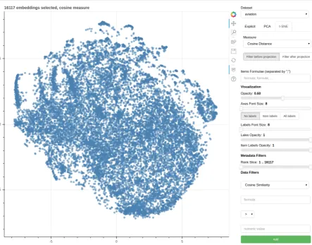
Figure 1: Screenshot of Parallax.
In this paper, we introduce Parallax, a tool for visualizing embedding spaces. The most widely adopted projection techniques (Principal Com-ponent Analysis (PCA) (Pearson, 1901) and t-Distributed Stochastic Neighbor Embedding (t-SNE) (van der Maaten and Hinton, 2008)) are available in Parallax. They are useful for obtaining an overall view of the embedding space, but they have a few shortcomings: 1) projections may not preserve distance in the original space, 2) they are not comparable across models and 3) do not pro-vide interpretable axes, preventing more detailed analysis and understanding.
t-SNE, differently from PCA, optimizes a loss that encourages embeddings that are in their re-spective close neighborhoods in the original high-dimensional space to be close in the lower di-mensional projection space. t-SNE projections vi-sually approximate better the original embedding space and topical clusters are more clearly distin-guishable, but do not solve the issue of compara-bility of two different sets of embeddings, nor do they solve the lack of interpretability of the axes or allow for fine-grained inspection.
For these reasons, there is value in mapping em-beddings into a more specific, controllable and in-terpretable semantic space. In this paper, a new and simple method to inspect, explore and debug embedding spaces at a fine-grained level is pro-posed. This technique is made available in Par-allax alongside PCA and t-SNE for goal-oriented analysis of the embedding spaces. It consists of explicitly defining the axes of projection through formulae in vector algebra that use embedding la-bels as atoms. Explicit axis definition assigns in-terpretable and fine-grained semantics to the axes of projection. This makes it possible to analyze in detail how embeddings relate to each other with respect to interpretable dimensions of variability, as carefully crafted formulas can map (to a certain extent) to semantically meaningful portions of the space. The explicit axes definition also allows for the comparison of embeddings obtained from dif-ferent datasets, as long as they have common la-bels and are equally normalized.
We demonstrate three visualizations that Par-allax provides for analyzing subspaces of inter-est of embedding spaces and a set of example case studies including bias detection, polysemy analysis and fine-grained embedding analysis, but additional ones, like diachronic analysis and the analysis of representations obtained through graph learning or any other means, may be performed as easily. Moreover, the proposed visualizations can be used for debugging purposes and, in general, for obtaining a better understanding of the embed-ding spaces learned by different models and rep-resentation learning approaches. We show how this methodology can be widely used through a series of case studies on well known models and data, and furthermore, we validate its usefulness for goal-oriented analysis through a user study.
Parallax interface, shown in Figure1, presents a plot on the left side (scatter or polar) and controls
[image:2.595.332.496.262.593.2]on the right side that allow users to define parame-ters of the projection (what measure to use, values for the hyperparameters, the formuale for the axes in case of explicit axes projections are selected, etc.) and additional filtering and visualization pa-rameters. Filtering parameters define logic rules applied to embeddings metadata to decide which of them should be visualized, e.g., the user can de-cide to visualize only the most frequent words or only verbs if metadata about part-of-speech tags is made available. Filters on the embeddings them-selves can also be defined, e.g., the user can decide to visualize only the embeddings with cosine sim-ilarity above 0.5 to the embedding of “horse”.
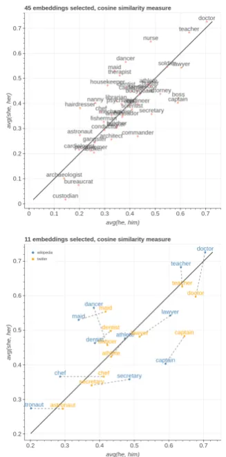
Figure 2: In the top we show professions plotted on “male” and “female” axes inW ikipediaembeddings. In the bottom we show their comparison inW ikipedia
andT witterdatasets.
(up to three) and potentially many items of inter-est, a Cartesian view is ideal. Each axis is the vec-tor obtained by evaluating the algebraic formula it is associated with, and the coordinates displayed are similarities or distances of the items with re-spect to each axis. Figure2shows an example of a bi-dimensional Cartesian view. In the case where the goal is defined in terms of many dimensions of variability, a polar view is preferred. The polar view can visualize many more axes by showing them in a circle, but it is limited in the number of items it can display, as each item will be displayed as a polygon with each vertex lying on a differ-ent axis and too many overlapping polygons would make the visualization cluttered. Figure5 shows an example of a five-dimensional polar view.
The use of explicit axes allows for interpretable comparison of different embedding spaces, trained on different corpora or on the same corpora but with different models, or even trained on two dif-ferent time slices of the same corpora. The only requirement for embedding spaces to be compara-ble is that they contain embeddings for all labels present in the formulae defining the axes. More-over, embeddings in the two spaces do not need to be of the same dimension, but they need to be normalized. Items will now have two sets of co-ordinates, one for each embedding space, and thus they will be displayed as lines. Short lines are in-terpreted as items being embedded similarly in the subspaces defined by the axes in both embedding spaces, while long lines are interpreted as really different locations in the subspaces, and their di-rection gives insight on how items shift in the two subspaces. The bottom side of Figure2shows an example of how to use the Cartesian comparison view to compare embeddings in two datasets.
2 Case Studies
In this section, a few goal-oriented use cases are presented, but Parallax’s flexiblity allows for many others. We used 50-dimensional publicly avail-able GloVe (Pennington et al.,2014) embeddings trained on Wikipedia and Gigaword 5 summing to 6 billion tokens (for shortWikipedia) and 2 billion tweets containing 27 billion tokens (Twitter).
Bias detection The task of bias detection is to identify, and in some cases correct for, bias in data that is reflected in the embeddings trained on such data. Studies have shown how embeddings incor-porate gender and ethnic biases ((Garg et al.,2018;
Bolukbasi et al.,2016;Islam et al.,2017)), while other studies focused on warping spaces in order to de-bias the resulting embeddings ((Bolukbasi et al.,2016;Zhao et al.,2017)). We show how our proposed methodology can help visualize biases.
To visualize gender bias with respect to pro-fessions, the goal is defined with the formulae
avg(he, him) and avg(she, her) as two dimen-sions of variability, in a similar vein to (Garg et al., 2018). A subset of the professions used by (Bolukbasi et al., 2016) is selected as items and cosine similarity is adopted as the measure for the projection. The Cartesian view visualizing
Wikipediaembeddings is shown in the left of Fig-ure2.Nurse,dancer, andmaidare the professions closer to the “female” axis, while boss, captain, andcommanderend up closer to the “male” axis.
The Cartesian comparison view comparing the embeddings trained on Wikipedia and Twitter is shown in the right side of Figure2. Only the em-beddings with a line length above 0.05 are dis-played. The most interesting words in this visual-ization are the ones that shift the most in the direc-tion of negative slope. In this case,chef and doc-torare closer to the “male” axis inTwitterthan in
Wikipedia, while dancer andsecretary are closer to the bisector inTwitterthan inWikipedia.
Polysemy analysis Methods for representing words with multiple vectors by clustering con-texts have been proposed (Huang et al.,2012; Nee-lakantan et al.,2014), but widely used pre-trained vectors conflate meanings in the same embedding.
Widdows(2003) showed how using a binary or-thonormalization operator that has ties with the quantum logicnotoperator it is possible to remove part of the conflated meaning from the embedding of a polysemous word. The authors define the op-eratornqnot(a, b) = a− a·b
|b|2band we show with
a comparison plot how it can help distinguish the different meanings of a word.
Figure 3: Plot of embeddings inWikipediawithsuitnegated with respect tolawsuitanddressrespectively as axes.
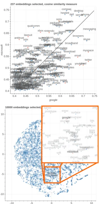
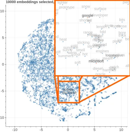
Figure 4: The top figure is a fine-grained comparison of the subspace on the axis google and microsoft in Wikipedia, the bottom one is thet-SNEcounterpart.
while words closer to the axis negatingdressare related to law. This visualization clearly confirms the ability of the nqnot operator to disentangle multiple meanings from polysemous embeddings.
Fine-grained embedding analysis We consider embeddings that are close to be semantically re-lated, but even close embeddings may have nu-ances that distinguish them. When projecting in two dimensions through PCA or t-SNE we are conflating a multidimensional notion of
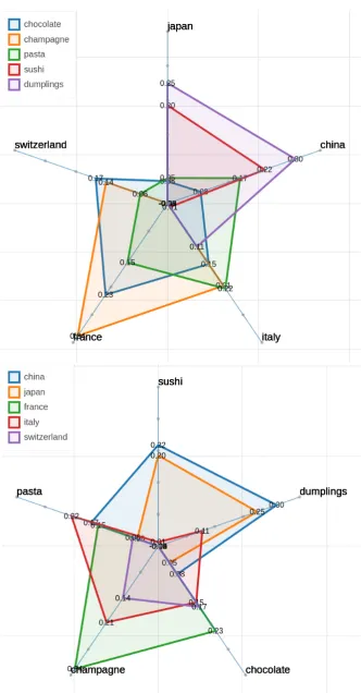
similar-Figure 5: Two polar views of countries and foods.
ity to a bi-dimensional one, losing the fine-grained distinctions. The Cartesian view allows for a more fine-grained visualization that emphasizes nuances that could otherwise go unnoticed.
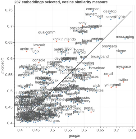
To demonstrate this capability, we select as dimensions of variability single words in close vicinity to each other in theWikipediaembedding space:googleandmicrosoft, asgoogleis the clos-est word tomicrosoftandmicrosoftis the 3rd clos-est word togoogle. As items, we pick the 30,000 most frequent words removing stop-words and re-move the 500 most frequent words (as they are too generic) and keeping only the words that have a cosine similarity of at least0.4 with bothgoogle
andmicrosoft and a cosine similarity below0.75
with respect togoogle+microsof t, as we are in-terested in the most polarized words.
The left side of Figure 4 shows how even if those embeddings are close to each other, it is easy to identify peculiar words (highlighted with red dots). The ones that relate to web companies and services (twitter,youtube,myspace) are much closer to the google axis. Words related to both legal issues (lawsuit, antitrust) and videogames (ps3,nintendo,xbox) and traditional IT companies are closer to themicrosoftaxis.
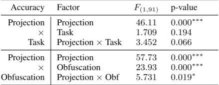
[image:4.595.95.267.214.567.2] [image:4.595.316.518.214.309.2]em-Accuracy Factor F(1,91) p-value
Projection Projection 46.11 0.000∗∗∗
× Task 1.709 0.194 Task Projection×Task 3.452 0.066
Projection Projection 57.73 0.000∗∗∗
[image:5.595.71.291.50.136.2]× Obfuscation 23.93 0.000∗∗∗ Obfuscation Projection×Obf 5.731 0.019∗
Table 1: Two-way ANOVA analyses of Task (Com-monality vs. Polarization) and Obfuscation (Obfus-cated vs. Non-obfus(Obfus-cated) over Projection (Explicit Formulae vs. t-SNE).
bedding space hides many nuances that are cap-tured in those representations, and on the other hand, that the proposed methodology enables for a more detailed inspection of the embedded space. Multi-dimensional similarity nuances can be vi-sualized using the polar view. In Figure 5, we show how to use Parallax to visualize a small num-ber of items on more than two axes, specifically five food-related items compared over five coun-tries’ axes. The most typical food from a spe-cific country is the closest to the country axis, withsushibeing predominantly close toJapanand
China,dumplingsbeing close to both Asian coun-tries andItaly,pastabeing predominantly closer to
Italy,chocolatebeing close to European countries andchampagnebeing closer toFranceandItaly. This same approach could be also be used for bias detection among different ethnicities, for instance.
3 User Study
We conducted a user study to find out if and how visualizations using user-defined semanti-cally meaningful algebraic formulae help users achieve their analysis goals. What we are not test-ing for is the projection quality itself, as in PCA and t-SNE it is obtained algorithmically, while in our case it is explicitly defined by the user. We for-malized the research questions as: Q1) Does Ex-plicit Formulae outperform t-SNE in goal-oriented tasks? Q2) Which visualization do users prefer?
To answer these questions we invited twelve subjects among data scientists and machine learn-ing researchers, all acquainted with interpretlearn-ing dimensionality reduction results. We defined two types of tasks, namely Commonality and Polariza-tion, in which subjects were given a visualization together with a pair of words (used as axes in Ex-plicit Formulae or highlighted with a big font and red dot in case of t-SNE). We asked the subjects to identify either common or polarized words w.r.t. the two provided ones. The provided pairs were:
banana & strawberry, google & microsoft, nerd & geek, book & magazine. The test subjects were given a list of eight questions, four per task type, and their proposed lists of five words are compared with a gold standard provided by a committee of two computational linguistics experts. The tasks are fully randomized within the subject to prevent from learning effects. In addition, we obfuscated half of our questions by replacing the words with a random numeric ID to prevent prior knowledge from affecting the judgment. We track the accu-racyof the subjects by calculating the number of words provided that are present in the gold stan-dard set, and we also collected an overall prefer-encefor either visualizations.
As reported in Table 1, two-way ANOVA tests revealed significant differences in accuracy for the factor of Projection and t-SNE against both Task and Obfuscation, which is a strong indicator that the proposed Explicit Formulae method outper-forms t-SNE in terms of accuracy in both Com-monality and Polarization tasks. We also observed significant differences in Obfuscation: subjects tend to have better accuracy when the words are not obfuscated. We run post-hoc t-tests that con-firmed how the accuracy of Explicit Formulae on Non-obfuscated is significantly better than Obfus-cated, which in turn is significantly better that t-SNE Non-obfuscated, which is significantly better than t-SNE Obfuscated. Concerning Preference, nine out of all twelve (75%) subjects chose Ex-plicit Formulae over t-SNE. In conclusion, our an-swers to the research questions are that (Q1) Ex-plicit Formulae leads to better accuracy in goal-oriented tasks, (Q2) users prefer Explicit Formu-lae over t-SNE.
4 Related Work
con-structing topic hierarchies. ConceptVector (Park et al., 2018) makes use of multiple keyword sets to encode the relevance scores of documents and topics: positive words, negative words, and irrel-evant words. It allows users to select and build a concept iteratively. (Liu et al.,2018) display pairs of analogous words obtained through analogy by projecting them on a 2D plane obtained through a PCA and an SVM to find the plane that separates words on the two sides of the analogy. Besides word embeddings, visualization has been used to understand topic modeling (Chuang et al., 2012) and how topic models evolve over time (Havre et al.,2002). Compared to existing literature, our work allows for more fine-grained direct control over the conceptual axes and the filtering logic, al-lowing users to: 1) define concepts based on ex-plicit algebraic formulae beyond single keywords, 2) filter depending on metadata, 3) perform mul-tidimensional projections beyond the common 2D scatter plot view using the polar view, and 4) per-form comparisons between embeddings from dif-ferent data sources. Those features are absent in other proposed tools.
5 Conclusions
We presented Parallax, a tool for embedding visu-alization, and a simple methodology for projecting embeddings into lower-dimensional semantically-meaningful subspaces through explicit algebraic formulae. We showed how this approach al-lows goal-oriented analyses, more fine-grained and cross-dataset comparisons through a series of case studies and a user study.
References
Tolga Bolukbasi, Kai-Wei Chang, James Y. Zou, Venkatesh Saligrama, and Adam Tauman Kalai. 2016. Man is to computer programmer as woman is to homemaker? debiasing word embeddings. In NIPS, pages 4349–4357.
Alexander Budanitsky and Graeme Hirst. 2006. Eval-uating wordnet-based measures of lexical semantic relatedness. Comput. Ling., 32(1):13–47.
Jason Chuang, Christopher D. Manning, and Jeffrey Heer. 2012. Termite: visualization techniques for assessing textual topic models. InAVI, pages 74–77.
Nikhil Garg, Londa Schiebinger, Dan Jurafsky, and James Zou. 2018. Word embeddings quantify 100 years of gender and ethnic stereotypes.Proceedings of the National Academy of Sciences.
Susan Havre, Elizabeth G. Hetzler, Paul Whitney, and Lucy T. Nowell. 2002. Themeriver: Visualizing the-matic changes in large document collections. IEEE Trans. Vis. Comput. Graph., 8(1):9–20.
Florian Heimerl and Michael Gleicher. 2018. Interac-tive analysis of word vector embeddings. Comput.
Graph. Forum, 37(3):253–265.
Eric H. Huang, Richard Socher, Christopher D. Man-ning, and Andrew Y. Ng. 2012. Improving word representations via global context and multiple word prototypes. InACL.
Aylin Caliskan Islam, Joanna J. Bryson, and Arvind Narayanan. 2017. Semantics derived automatically from language corpora necessarily contain human biases. Science, 356:183–186.
Hanseung Lee, Jaeyeon Kihm, Jaegul Choo, John T. Stasko, and Haesun Park. 2012. ivisclustering: An interactive visual document clustering via topic modeling. Comput. Graph. Forum, 31(3):1155– 1164.
Alessandro Lenci. 2018. Distributional models of word meaning. Annual Review of Linguistics, 4(1):151– 171.
Shusen Liu, Peer-Timo Bremer, Jayaraman J. Thia-garajan, Vivek Srikumar, Bei Wang, Yarden Livnat, and Valerio Pascucci. 2018. Visual exploration of semantic relationships in neural word embeddings.
IEEE Trans. Vis. Comput. Graph., 24(1):553–562.
Laurens van der Maaten and Geoffrey Hinton. 2008. Visualizing data using t-SNE. Journal of Machine
Learning Research, 9:2579–2605.
Arvind Neelakantan, Jeevan Shankar, Alexandre Pas-sos, and Andrew McCallum. 2014. Efficient non-parametric estimation of multiple embeddings per word in vector space. InEMNLP, pages 1059–1069.
Deok Gun Park, Seungyeon Kim, Jurim Lee, Jaegul Choo, Nicholas Diakopoulos, and Niklas Elmqvist. 2018. Conceptvector: Text visual analytics via in-teractive lexicon building using word embedding.
IEEE Trans. Vis. Comput. Graph., 24(1):361–370.
K. Pearson. 1901. On lines and planes of closest fit to systems of points in space. Philosophical Magazine, 2:559–572.
Jeffrey Pennington, Richard Socher, and Christo-pher D. Manning. 2014. Glove: Global vectors for word representation. InEMNLP, pages 1532–1543.
Dominic Widdows. 2003. Orthogonal negation in vec-tor spaces for modelling word-meanings and docu-ment retrieval. InACL, pages 136–143.
A Appendix
Figure
9:
Plot
of
embeddings
in
W
ikipedia
with
suit
ne
g
ated
with
respect
to
lawsuit
and
dr
ess
respecti
v
ely
as
ax
Figure
10:
Plot
of
embeddings
in
W
ikipedia
with
apple
ne
g
ated
with
respect
to
fruit
and
computer
respecti
v
ely
as
ax
Figure
12:
Fine-grained
comparison
of
the
subspace
on
the
axis
nq
not
(
g
oog
le,
micr
osof
t
)
and
nq
not
(
micr
osof
t,
g
oog
le
)
in
W
ikipedia