An Evaluation of Singular Spectrum Analysis Based Seasonal Adjustment

Munich Personal RePEc Archive

An Evaluation of Singular Spectrum

Analysis-Based Seasonal Adjustment

Leon, Costas

15 February 2018

Online at

https://mpra.ub.uni-muenchen.de/84594/

1

An Evaluation of Singular Spectrum Analysis-Based Seasonal Adjustment Costas Leon1

ABSTRACT

In this paper, the Singular Spectrum Analysis (SSA) is presented and applied in the US

air traffic emplacements for the period Jan. 1954 – Sept. 2011. I decompose the US

air traffic emplacements in trend, cycle, seasonal and noise components. In turn, I apply several spectral criteria in order to evaluate the SSA as a seasonal adjustment filter. SSA detects, beyond trend, strong cycles and seasonal components and leaves as a residual a GARCH process. SSA performs quite well as a seasonal adjustment mechanism in the case of the GARCH process but it performs even better in the case of a simulated white noise process. SSA is a serious candidate in economics in dealing with filtering, denoising, smoothing and seasonal adjustment.

Keywords: Singular Spectrum Analysis, Seasonal Adjustment, Spectral Analysis, Economic Time Series, Air Traffic Emplacements.

1. INTRODUCTION

One of the important topics in economic time series analysis is a meaningful decomposition in unobserved components such as signal and noise. In the case that the interest of the analyst is the determination of a cyclical component, the usual approach is within the time domain and, because of this, spectral methods (i.e. the frequency domain) are comparatively few. I feel, however, that the “natural” way of the analysis of the economic cycle lies in the frequency domain, because of the “cyclical” properties of many economic time series. In this context, the Singular Spectrum Analysis (SSA) is a method that helps to obtain a better signal which, if desired, can be further processed by spectral methods.

SSA is a relatively new method of time series analysis and combines elements of various fields of studies such as, among others, statistics and probability theory, dynamical systems and signal processing. It is based on the spectral decomposition of time series (Karhunen, 1946 and Loève, 1978) and on the Mañé (1981) and Takens (1981) embedding theorem. Applications of SSA typically include hydrology, geophysics, climatology, biology, physics, and very recently macroeconomics and financial economics. SSA is model-free and data-adaptive method and depends only on one parameter, the window length (the embedding dimension). Therefore, SSA is relatively easy to understand and apply it. It gives remarkable results especially in short and noisy time series, as many economic time series are. The SSA was developed independently in 1980’s in the USA and UK under the name SSA and in the 1990’s in Russia (St. Petersburg and Moscow) under the name Caterpillar-SSA.

SSA exists both in univariate and multivariate versions with several variations (e.g. Basic SSA, sequential SSA, etc). Since this is a relatively new method, one expects

2

more methodological advances and practical applications in the near future. The central concept of SSA is the partitioning of a vector space into subspaces that have some meaningful interpretation, i.e. a decomposition of a time series in signal (such as trends, cycles and seasonal components) and noise.

In this paper, I present the application of the SSA method in the decomposition of US air traffic emplacements into trend, cycle, seasonal variation and noise. The US air traffic emplacements is defined as the number of onboard passengers on individual scheduled airline flights carried by US air carriers operating between airports located within the boundaries of the United States and its territories. Then the SSA is employed to obtain a seasonally adjusted time series. The evaluation of the SSA as a seasonal adjustment filter is examined next by means of several spectral criteria.

2. METHODOLOGICAL ASPECTS OF SSA

The SSA can be understood as the singular value decomposition of a matrix consisting of delayed vectors (the time series under consideration embedded into some integer dimension), called trajectory matrix, shown to be a Hankel matrix, and the regroupping of the obtained orthonormal vectors into a sets of meaningful, to the application at hand, components (subspaces) through the process of diagonal averaging. These sets in the macroeconomic analysis of the business cycle are the trend, the cycle, the seasonal components and the noise. This section describes the SSA algorithm used for extraction of the signals. SSA comprises of two main stages: decomposition and reconstruction. In turn, the decomposition stage comprises of two steps: embedding and singular value decomposition. The reconstruction stage comprises of two steps, too: grouping and diagonal averaging (or Hankelization). The

presentation below follows Beneki et al. (2011), Golyandina et al. (2001, Chapters 1

and 2), Hassani and Thomakos (2010) and Hassani and Zhigljavsky (2008).

2.1 Stage 1: Decomposition, Step 1: Embedding

Let . Consider a one-dimensional real-valued time series of

length N, a positive integer L (window length) such that and a mapping of

the original series into a sequence of L-dimensional lagged

vectors , , by the formula:

, The Hankel matrix X= of size is

called the L-trajectory matrix (or simply, the trajectory matrix) of the series F. In

linear algebra, a Hankel matrix is a matrix where all the elements along the diagonal

i+j=const. are equal. In other words, the trajectory matrix is

3

Note that if N and L are fixed, then there is a one-to–one correspondence between

Hankel matrices of size and time series of length N.

2.2 Stage 1: Decomposition, Step 2: Singular Value Decomposition (SVD)

The SSA is based on a particular transformation known in matrix algebra as singular

value decomposition (SVD). The SVD of the trajectory matrix X= is a

decomposition of X in the form X= , where XT _,

X, are the eigenvalues of the matrix S

= XXT _{taken inthe decreasing order of magnitude and}

are the eigenvectors of the matrix S corresponding to these eigenvalues. If we define

Xi= , then the SVD of the trajectory matrix can be written as a

sum of rank-one orthogonal matrices:

X=X1+…+Xd (1)

where are the orthonormal eigenvectors of S = XXT _{(in SSA terminology they are}

called empirical orthogonal functions) and (in SSA terminology they are called

principal components) can be regarded as the eigenvectors of the matrix XT_{X. The}

collection is called the i-th eigentriple of the matrix X,

are the singular values of the matrix X and , are the left and right singular

vectors of X,respectively. SVD is attractive because it ensures optimality. Among all

the matrices X(r) _{of rank r<d, the matrix provides the best approximation to}

the trajectory matrix X, so that is minimum. Note that and

for . Thus, we can consider the ratio as the contribution

of the matrix Xi in the expansion (1) to the whole trajectory matrix X. Consequently,

the sum of the first r ratios, is the contribution of the optimal

approximation of the trajectory matrix by the matrices of rank r.

2.3 Stage 2: Reconstruction, Step 1: Grouping

The grouping step corresponds to splitting the elementary matrices Xi into several

groups and summing the matrices within each group. Let be a group of

indices. Then the matrix XI corresponding to the group I is defined as XI = Xi1 + . . . +

Xip. These matrices are computed for I = I1, . . . , Imand the expansion (1)leads to the

decomposition

X = XI1 + . . . + XIm (2)

4

2.4 Stage 2: Reconstruction, Step 2: Diagonal Averaging

The last step is, in a sense, opposite to the first step and transforms each matrix of the grouped decomposition (2) into a system of new (reconstructed) series of length

N. This procedure is the so-called Hankelization or diagonal averaging. If zijstands for

an element of a matrix Z, then the k-th term of the resulting time series is obtained

by averaging zijover all i, j such that i + j = k + 2. The result of the Hankelization of a

matrix Z is the Hankel matrix HZ, which is the trajectory matrix corresponding to the

time series obtained as a result of the diagonal averaging (see the formal description

in Golyandina et al., op.cit.). Note that the Hankelization is an optimal procedure in

the sense that the matrix HZ is the closest to Z (with respect to the matrix norm)

among all Hankel matrices of the corresponding size (Golyandina et al.,op.cit.). In its

turn, the Hankel matrix HZ defines the series uniquely by relating the values in the

diagonals to the values in the series. Diagonal averaging applied to a matrix XIk

produces the series . Hence, the original series f0, ,...,f1 fN-1 is

decomposed into the sum of m series:

.

3. APPLICATION: DECOMPOSITION OF THE US AIR TRAFFIC EMPLACEMENTS

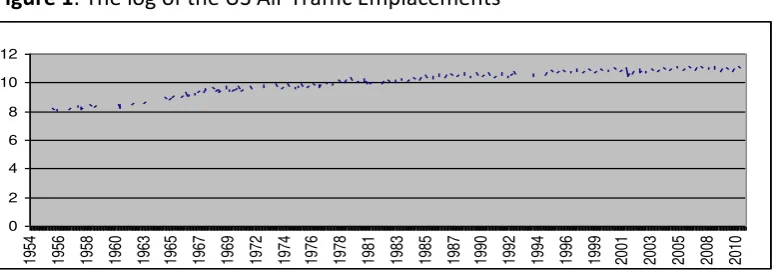
As an illustration, I apply the method to the US air traffic Emplacements. The data set consists of the natural logarithm (denoted by log) of this time series spanning the

period Jan. 1954 – Sept. 2011, i.e. 693 monthly, seasonally unadjusted observations.

Figure 1 displays the log (the natural logarithm) of the US air traffic emplacements.

Figure 1: The log of the US Air Traffic Emplacements

3.1 The Choice of the Window Length

As mentioned in the Introduction, SSA depends on one parameter, called window

length . should be large enough in order to capture sufficiently the dynamics of

the time series but not larger than . Further, if any periodic components are

known to be present in the time series, then should be proportional to the

longest, in wave length, period. Under the assumption of a local trend model (the signal in the state equation is hidden in noise in the observational equation), there is a relationship between the window length and the signal to noise ratio (S/N). As S/N

approaches zero, then the window length should converge to and as S/N

0 2 4 6 8 10 12

5

approaches infinity, then the window length should converge to . See Hassani

and Thomakos (2010). Spectral density or other relevant measures showing peaks in the dominant frequencies or exogenous information may assist in the determination of periodic components.

3.2 The Determination of the Signal Components

Once the window length has been determined, some other information might be valuable in order to proceed to the grouping step of the reconstruction stage. For example, in practice, a periodic component is identified by having two eigentriples with singular values close each other (the exception is at frequency 0.5 which displays one eigentriple with saw-tooth singular vector). Therefore, a plot of the

singular values against an index i=1,…,L, gives important information in the

sense that , through this visual aid, one can easily discern the high and the low

singular values. Since each singular value expresses the significance of the

corresponding to the total trajectory matrix , high singular values imply

significance of the corresponding eigentriple as a determinant of the variance of the time series.

3.3 Decomposition and Reconstruction

Based on the above considerations, having no further information about the S/N ratio (which could be measured, for example, by the Kalman filter), and on the basis of a preliminary spectral estimation (not shown), a window length of 144 has been determined, reflecting a cycle of 12 years (12 years x 12 months=144).

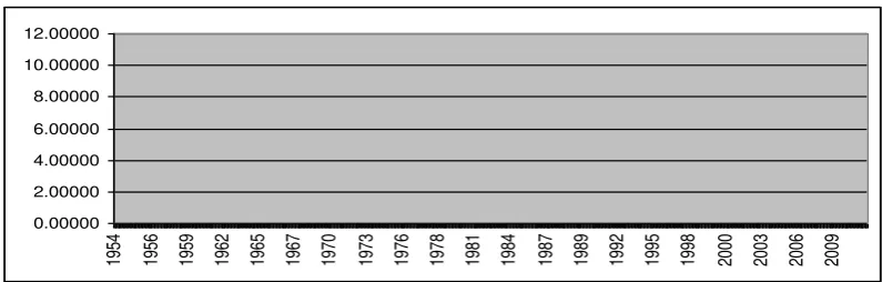
3.3.1 The Long-Run Trend

The long-run trend is reconstructed on the basis of the first and second eigentriple, Figure 2.

Figure 2: The Long-Run Trend

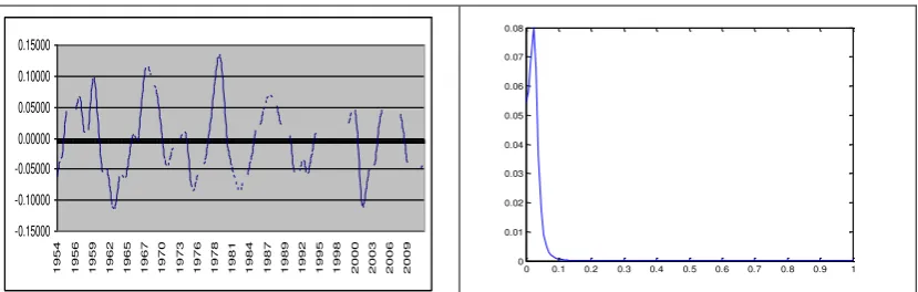
3.3.2 The Cycle

The cycle consists of the eigentriples 5-6, 11-13, 20-23, 26-27. The volatility of the cycle is strong and varies between -11% to 13% relative to trend. The spectral density, obtained by the maximum entropy estimator (Burg, 1975) with an AR(4), provides a sharp peak at a frequency corresponding to 12 years, Figure 3.

0.00000 2.00000 4.00000 6.00000 8.00000 10.00000 12.00000

6 Figure 3: The Cycle and its Spectrum

0 0.1 0.2 0.3 0.4 0.5 0.6 0.7 0.8 0.9 1

0 0.01 0.02 0.03 0.04 0.05 0.06 0.07 0.08

3.3.3 The Seasonal Component

The seasonal component is reconstructed according to the eigentriples 3-4, 7-10, 16-19. Figure 4 shows the reconstructed seasonal component. The seasonal component is very strong, varying from -15% to 15% relative to trend.

Figure 4: The Reconstructed Seasonal Component

3.3.4 The Noise

The noise component is reconstructed on the basis of the remaining eigentriples. Figure 5 shows the reconstructed noise. In Figure 6 the comparison between the distribution of the residuals of the variance equation of a fitted GARCH (1,1) model in the reconstructed noise and its corresponding theoretical normal distribution are shown.

Figure 5: The Reconstructed Noise

-0,20000 -0,15000 -0,10000 -0,05000 0,00000 0,05000 0,10000 0,15000 0,20000

1954 1956 1959 1962 1965 1967 1970 1973 1976 1978 1981 1984 1987 1989 1992 1995 1998 2000 2003 2006 2009

-0.15000 -0.10000 -0.05000 0.00000 0.05000 0.10000 0.15000

1954 1956 1959 1962 1965 1967 1970 1973 1976 1978 1981 1984 1987 1989 1992 1995 1998 2000 2003 2006 2009

-0.10000 -0.08000 -0.06000 -0.04000 -0.02000 0.00000 0.02000 0.04000 0.06000 0.08000

7

Figure 6: Comparison of the Distributions of the Residuals in the Variance Equation to the Normal Distribution

-6 -4 -2 0 2 4 6

-.15 -.10 -.05 .00 .05 .10 .15

Resi duals of the Vari ance Equati on

Nor

mal

Qu

anti

le

Theoreti cal Quantile-Quanti le

3.3.5 The Reconstructed Air Traffic Emplacements

Based on the decomposition of the air traffic emplacements into the three subsignals of interest (trend, cycle and seasonal variation), I now proceed to the reconstruction of the air traffic emplacements (i.e. signal = trend + cycle + seasonal variation = actual air traffic emplacements - noise). The signal is displayed in Figure 7.

Figure 7: The Reconstructed Air Traffic Emplacements Signal

0.00000 2.00000 4.00000 6.00000 8.00000 10.00000 12.00000

1954 1956 1958 1961 1963 1966 1968 1970 1973 1975 1978 1980 1983 1985 1987 1990 1992 1995 1997 1999 2002 2004 2007 2009

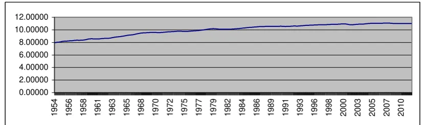
3.3.6 The Seasonally Adjusted Air Traffic Emplacements

Since the signal in Figure 7 contains the seasonal component, seasonal adjustment can easily be made by reconstructing a time series which contains only the trend and the cycle. This could be considered as seasonally adjusted time series (without the noise). The seasonally adjusted air traffic emplacements signal is displayed in Figure 8.

Figure 8: The Seasonally Adjusted Air Traffic Emplacements

0.00000 2.00000 4.00000 6.00000 8.00000 10.00000 12.00000

8

3.4 SSA-Based Seasonal Adjustment: An Evaluation

In the literature of seasonal adjustment there are some criteria, according to which a seasonal adjustment procedure is characterized as good. I follow Rosenblat (1968) who presents a series of spectral criteria for a good seasonal adjustment. The criteria refer to the spectrum, coherence and phase between the unadjusted and the seasonally adjusted time series as well as to the spectrum and the coherence between the noise and the seasonally adjusted series and the cospectrum between the trend-cycle and the noise. In particular, the criteria are as follows:

A: Criteria between the Adjusted and Unadjusted Series

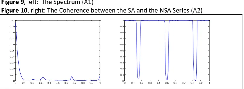
A1. The spectrum of a stationary non-cyclical seasonally adjusted series is relatively

flat with no dominant peaks or troughs at the seasonal periods of 12/k months (i.e.

at seasonal frequencies 2πk/12), k= 1,2,...,6. A cyclical and seasonally adjusted series

presents a spike in the low frequency band and very low, insignificant, spikes in the seasonal frequencies. This criterion is fulfilled. Figure 9.

A2. The coherence between the seasonally adjusted and unadjusted series should be

very low at seasonal frequencies but should be high at non seasonal frequencies although the coherence may be reduced if significant moving seasonality is present. This criterion is fulfilled. Figure 10.

Figure 9, left: The Spectrum (A1)

Figure10, right: The Coherence between the SA and the NSA Series (A2)

0 0.1 0.2 0.3 0.4 0.5 0.6 0.7 0.8 0.9 1

0 0.01 0.02 0.03 0.04 0.05 0.06 0.07 0.08 0.09 0.1

0 0.1 0.2 0.3 0.4 0.5 0.6 0.7 0.8 0.9 1

0 0.1 0.2 0.3 0.4 0.5 0.6 0.7 0.8 0.9 1

Note: SA: seasonally adjusted, NSA: non-seasonally adjusted.

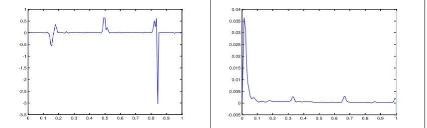
A3. The phase spectrum between the seasonally adjusted and the unadjusted series

should be ideally zero or close to zero although large deviations from zero might be expected at seasonal frequencies due to sampling properties of the phase estimates. In the high frequency, the phase is rather large. This criterion is partially fulfilled. Figure 11.

A4. The cospectrum between the seasonally adjusted and the unadjusted series

9

Figure 11, left: The Phase Spectrum between the SA and the NSA Series (A3) Figure 12, right: The Cospectrum between the SA and the NSA Series (A4)

0 0.1 0.2 0.3 0.4 0.5 0.6 0.7 0.8 0.9 1

-3.5 -3 -2.5 -2 -1.5 -1 -0.5 0 0.5 1

0 0.1 0.2 0.3 0.4 0.5 0.6 0.7 0.8 0.9 1

-0.005 0 0.005 0.01 0.015 0.02 0.025 0.03 0.035 0.04

Note: SA: seasonally adjusted, NSA: non-seasonally adjusted.

B. Criteria between the Adjusted Series and the Noise

B1. The spectrum of the noise should be relatively flat over the whole range of

frequencies. This criterion is not fulfilled. Figure 13.

B2. Over the frequency range 2π/12 to π (12 to 2 months) the spectrum of the non -cyclical, seasonally adjusted series and the noise should be similar in appearance, in that they have the same spectral power, both being relatively flat. In a cyclical series, only the spikes at the low frequencies dominate. This criterion is fulfilled. Figure 14.

Figure 13,left: The Spectrum of the Noise (B1)

Figure 14,right: The Spectra of the SA Series and the Noise (B2)

0 0.1 0.2 0.3 0.4 0.5 0.6 0.7 0.8 0.9 1

0.6 0.8 1 1.2 1.4 1.6 1.8 2 2.2 2.4

2.6x 10

-3

0 0.1 0.2 0.3 0.4 0.5 0.6 0.7 0.8 0.9 1 0.6 0.8 1 1.2 1.4 1.6 1.8 2 2.2 2.4 2.6x 10-3

0 0.1 0.2 0.3 0.4 0.5 0.6 0.7 0.8 0.9 1 0 0.005 0.01 0.015 0.02 0.025 0.03 0.035 0.04

Note: SA: seasonally adjusted.

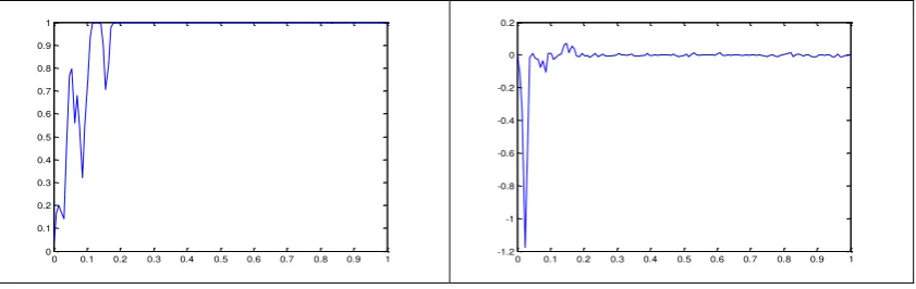
B3. Over the frequency range 2π/12 to π (12 to 2 months) the coherence between

the noise and the seasonally adjusted series should be very high and the phase should be ideally zero or close to zero. For periods higher than 12 months, the coherence should be zero and the phase arbitrary. This criterion is fulfilled. Figure 15.

10

0 0.1 0.2 0.3 0.4 0.5 0.6 0.7 0.8 0.9 1

0 0.1 0.2 0.3 0.4 0.5 0.6 0.7 0.8 0.9 1

0 0.1 0.2 0.3 0.4 0.5 0.6 0.7 0.8 0.9 1

-1.2 -1 -0.8 -0.6 -0.4 -0.2 0 0.2

B4. The trend-cycle series and the noise should have zero cospectrum over all

frequency range except the very low frequency band. This criterion is partially fulfilled. Figure 16.

Figure 16: The Cospectrum of the SA Series and the Noise (B4)

0 0.1 0.2 0.3 0.4 0.5 0.6 0.7 0.8 0.9 1

-4 -3 -2 -1 0 1 2 3 4

5x 10

-3

Note: SA: seasonally adjusted.

From the visual examination of Figures 9-16, 4 criteria (A1, A2, B2, B3) are fully met, 3 (A3, A4, B4) were partially met and 1 (B1) was not met. As for the criterion B1, this was expected since the noise component is governed by a GARCH (1,1) process. However, in the case of a simulated white noise (not shown here), the criteria B1 and B4 are fully met (Beneki and Leon, 2012).

4. CONCLUSION

11 REFERENCES

Beneki, C., Eeckels, B., Leon, C. (2011), “Signal Extraction and Forecasting of the UK

Tourism Income Time Series. A Singular Spectrum Approach.” Journal of Forecasting,

9 March 2011, DOI:10:1002/for.1220.

Beneki, C., Leon, C. (2011) “Evaluation of Singular Spectrum Analysis-Based Seasonal

Adjustment Procedure”. The 2012 International Conference on the Singular

Spectrum Analysis and its Applications, Beijing, China, 17-20 May 2012.

Burg, J.P., Maximum Entropy Spectral Analysis, PhD Thesis, Stanford University, 1975.

Golyandina, N., Nekrutkin, V., Zhigli︠a︡vskiĭ, A. Analysis of Time Series Structure: SSA and Related Techniques, Chapman and Hall/CRC, 2001.

Hassani, H., Thomakos, D. (2010). “A Review on Singular Spectrum Analysis for

Economic and Financial Time Series”,Statistics and Its Interface, Forthcoming.

Karhunen, K. Zur Spektraltheorie Stochastischer Prozesse, Ann. Acad. Sci. Fenn. Ser. A1, Math. Phys., 34, 1946.

Loève, M.: Probability Theory, Vol. II, 4th ed., Springer-Verlag, 1978.

Mañé, R., (1981), “On the dimension of the compact invariant sets of certain nonlinear maps”, in Dynamical Systems and Turbulence, Eds. D. A. Rand and L. S.

Young, Springer-Verlag, New York, 230–242.

Rosenblat, H.M, (1968), Spectral Evaluation of BLS and CENSUS Revised Seasonal

Adjustment Procedures. J. Amer. Stat. Assoc., 63: 472-501)

Takens, F., (1981), “Detecting strange attractors in turbulence”. In Dynamical Systems and Turbulence, D. A. Rand and L.-S. Young (Eds.), Springer-Verlag, New