Modeling Plume Rise of Air Emissions from Animal Housing Systems: Inverse AERMOD

(1)

http://www.scirp.org/journal/jep ISSN Online: 2152-2219

ISSN Print: 2152-2197

DOI: 10.4236/jep.2017.811078 Oct. 19, 2017 1254 Journal of Environmental Protection

Modeling Plume-Rise of Air Emissions from

Animal Housing Systems: Inverse AERMOD

Manqing Ying1, Lingjuan Wang-Li1*, Larry F. Stikeleather1, Jack Edwards2

1_{Department of Biological and Agricultural Engineering, North Carolina State University, Raleigh, USA} 2_{Department of Mechanical and Aerospace Engineering, North Carolina State University, Raleigh, USA}

Abstract

As fate and transport of air emissions from animal housing systems is of in-creasing concern, dispersion models have become commonly used tools to es-timate the downwind concentrations of pollutants at certain locations sur-rounding the animal production farms. In application of Gaussian dispersion model for downwind concentration predictions of animal housing emissions, unknown plume rise (△h) and plume shape of the horizontally emitted plumes from animal housing systems have been vital weak points challenging the accuracy of the model predictions. This paper reports an inverse AERMOD modeling study to derive the plum rises of PM10 emissions from mechanically ventilated egg production houses based upon field measurements of PM10 emission rate, downwind concentrations, and meteorological conditions. In total, 87 hourly plume rises were found for 20 days (five days per season for four seasons, from fall 2008 to summer 2009). The mean plume rises for fall 2008, winter 2008, spring 2009 and summer 2009 were 16.2 m (SE = 11.2 m), 7.9 m (SE = 9.5 m), 16.5 m (SE = 12.4 m), and 14.3 m (SE = 10.0 m), respec-tively. The relationships between plume rises and various factors were tested. While the diurnal patterns of the plume rises were not consistent among dif-ferent selective days, they generally followed the diurnal patterns of house ventilation rates. Plume rise for weekends were significantly higher than those for weekdays in fall. Multiple linear regression showed a significant positive relationship (p = 0.0134) between wind speed and the plume rises. Ambient relative humidity and total volume flow were also found to be slightly (p = 0.171 and 0.217, respectively) related to the plume rises.

Keywords

Animal Feeding Operation, Air Emission, Plume-Rise, AERMOD

How to cite this paper: Ying, M.Q., Wang-Li, L., Stikeleather, L.F. and Ed-wards, J. (2017) Modeling Plume-Rise of Air Emissions from Animal Housing Sys-tems: Inverse AERMOD. Journal of Envi-ronmental Protection, 8, 1254-1269.

https://doi.org/10.4236/jep.2017.811078

Received: August 21, 2017 Accepted: October 16, 2017 Published: October 19, 2017

http://creativecommons.org/licenses/by/4.0/

(2)

DOI: 10.4236/jep.2017.811078 1255 Journal of Environmental Protection

1. Introduction

Animal feeding operations (AFOs) emit significant amount aerial pollutants, contributing to the elevated air pollutant concentrations in the vicinity areas

[1]-[9]. Although air emissions from AFOs are of great environmental concern in

the United States (U.S.), application of the current National Ambient Air Quality Standards (NAAQS) is challenged due to lack of knowledge about air dispersions of AFO air emissions. Fate and transport of air emissions from AFO facilities have become a growing political and environmental concern [10] [11] [12].

In the studies of AFOs air emissions, atmospheric dispersion models are often used to predict downwind concentrations of the emitted pollutants [13]-[19], or, to derive emission rates through inverse modeling [20]-[26]. Among various types of dispersion models (e.g., Box models, Gaussian models, Lagrangian and Eulerian models, and CFD model) [27], Gaussian plume models are the most widely used for numerically describing dispersion of air emissions from different types of sources (e.g., point, line, area, volume; or, industrial stacks versus agri-cultural operations; etc.) [28] [29] [30] [31]. In application of the Gaussian persion models, knowledge about plume-rise is required for simulating the dis-persion of the plume and calculating the concentrations at downwind locations

[28] [32] [33] [34]. By definition, plume rise is the rise of the dispersing plume

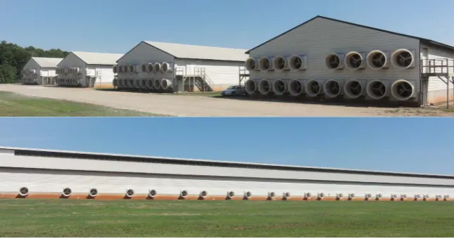
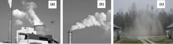
centerline above its original emission source height (i.e., the physical stack height). In the literature, dispersion plume rises from various emission sources have been experimentally studied [35]-[42] and several plume rise models were developed from observations of emission plumes from industrial stacks (Figure 1(a) & Figure 1(b)) with both vertical momentum and thermal buoyancy [32]

[43] [44] [45] [46] [47]. In modern animal production houses, mechanical

ven-tilation systems are used to create optimal growing conditions for animals. Aeri-al pollutants from those houses are usuAeri-ally released through ventilation fans at ground level and horizontal positions or positions slightly tipping downwards

(Figure 1(c)). There is no actual emission “stack”, nor is there upward vertical

[image:2.595.210.539.593.677.2]

velocity. As a result, the current plume rise models do not apply for AFO air emission dispersion modeling. Unknown plume-rise and plume shape (i.e., ho-rizontal and vertical plume spread parameters) are vital weak points challenging the accuracy of the Gaussian model predictions.

(3)

As a preferred regulatory air dispersion model of the U.S. Environmental Protection Agency (EPA), AERMOD was developed by the American Meteoro-logical Society (AMS) and EPA Regulatory Model Improvement Committee (AERMIC) in early 1990’s. This AERMIC Model (i.e., AERMOD) was a re-placement of the previous regulatory model ISCST3. Like ISCST3, AERMOD is a Gaussian-based model that incorporates advanced understanding of the boundary theory and turbulence with inclusion of terrain interactions [48] [49] [50]. In AERMOD, at stable conditions, the plume dispersion is treated as Gaus-sian distribution in both vertical and horizontal directions; the plume rise is de-termined by Briggs equations [48] [49] that takes temperature and wind changes above stack top into consideration. At unstable conditions (convective contions), the plume dispersion is treated as Gaussian distribution in horizontal di-rection and as bi-Gaussian probability distribution in vertical didi-rection; the plume rise is determined using convective plume rise formulations that account for convective updrafts and downdrafts [48] [49]. Although AERMOD is far more advanced than other Gaussian-based models, it still shares the deficiency in assessing the plum rise for emission sources with ground level and horizontal emission characteristics as it is of animal housing emission. Since AERMOD has been adopted by the State Air Pollution Regulatory Agencies (SAPRAs) to pre-dict downwind concentrations or to derive emission rates through inverse mod-eling, and/or to compile emission inventories for agricultural emission sources, it is essential to develop understand the dynamics of the plume rises of agricultural air emissions as impacted by the production practices and atmospheric conditions. Therefore, the objectives of this research were to apply inverse-AERMOD to de-rive the plume rises of animal house air emissions using field measurements of particulate matter (PM) emissions and downwind concentrations; and to identi-fy the impacts of various factors on plume rises from the animal houses based upon the inverse-AERMOD results and the field observations.

2. Materials and Methods

In this study, plume rises for animal housing systems were predicted using in-verse AERMOD approach. The PM10 dispersion from a commercial egg produc-tion farm was modeled based upon measured emission rates. The plume rises for the source types (i.e., ventilation types) were adjusted and the results of model predicted hourly downwind PM10 concentrations were compared with field ob-servations at four ambient stations in the vicinity. When the model prediction agreed with the field measurement within ±20% relative difference, the plume rise for that given hour was considered valid. In total, 480 hourly PM10 data for four seasons with five days per season for four seasons were selected for this modeling study.

2.1. The Egg Production Farm and the PM10 Monitoring Station

(4)

North Carolina. As shown in Figure 2, this farm consisted of nine layer houses and an egg packing building. Based on the house type and ventilation type, the production houses were grouped into (1 tunnel ventilated high-rise layer houses (houses 1 - 4); (2 cross ventilated high-rise layer houses (houses 5 - 6); and (3 naturally ventilated shallow pit layer houses (houses 93, 102 - 103). In the high-rise houses, laying hens were caged on the second floor in 6 rows (houses 1 - 4) or 8 rows (houses 5 - 6) and manure was stored in the first floor and was completely cleaned out once a year. In the naturally ventilated houses, hens were caged in 4 tires and manure was flushing out to lagoons twice a day. The dimen-sions of the houses are listed in Table 1.

The tunnel ventilated houses used 17 belt-driven ventilation fans (upper 8 and lower 9, 1.22 m in diameter) on end wall of each house (Figure 3). The cross- ventilated houses had 27 belt-driven ventilation fans (1.22 m in diameter) ar-rayed on each side wall of each house (Figure 3). The naturally ventilated had curtain openings on the side walls, and twenty winter vents evenly distributed on the building ridge.

The PM concentrations were monitored at 5 locations, of which one was the in-house monitoring station (ST1 in Figure 2) and 4 were ambient monitoring

[image:4.595.208.540.348.531.2]

ST1 = station 1 (inside the house 4); ST2 = station 2; ST3 = station 3; ST4 = station 4; ST5 = station 5

Figure 2. The egg production farm layout and the PM10 monitoring stations [51].

Table 1. Building information of the production houses.

House Length (m) Width (m) Height (m) Ventilation type Hen population

1 - 4 176.8 17.8 _{8.4 (ridge)}5.5 (eave) Tunnel ~96,000 per house

5 - 6 176.8 21.0 _{8.4 (ridge)}5.5 (eave) Cross ~130,000 per house

102 - 103 152.4 17.8 _{5.5 (ridge)}3.0 (eave) Nature ~70,000 per house

[image:4.595.201.539.593.731.2]

(5)

DOI: 10.4236/jep.2017.811078 1258 Journal of Environmental Protection Figure 3. Illustration of the fans in tunnel-ventilated houses (top) & a cross-ventilated house (bottom).

stations (ST2-5 in Figure 2). The ST1 was designed to measure in-house PM concentration for determination of PM emission rate from the tunnel ventilated houses, whereas ST2-5 were designed to simultaneously measure downwind and upwind PM concentrations. Also, there is another PM monitor at the ventilation air inlet of house 4, measuring the background PM concentrations of the house inlet air. At each PM monitoring station, one tapered element oscillating micro-balance (TEOM) equipped with a federal reference method PM10 sampling head was used to take continuous PM10 measurements [5] [51]. A 10 m weather tower with sensors for solar radiation, wind speed and direction, ambient temperature and relative humidity (RH) were used to take onsite meteorological measure-ments at one minute interval.

In this study, dispersion modeling was conducted based upon hourly mea-surement data for four periods with each period having consecutive five days from fall 2008 to summer 2009. Dates with rainfall, snowfall or other unusual conditions (e.g., instrument calibration dates) were excluded. The selection of the five days was set to be the periods with the least data points being excluded. In total, 435 valid hours were finally selected for the modeling practices.

2.2. AEROMOD Simulation

2.2.1 PM10 Emission Rate Determination

For tunnel-ventilated houses, the PM10 emission rate (ER) of house 4 was calcu-lated based upon field measurements of PM10 concentration and house ventila-tion rate using Equaventila-tion (1) [5] The ERs from other three tunnel houses (1 - 3) were assumed to be the same as it from the house 4 since these four houses were identical in building configurations, ventilation system controls, production management practices, and hen types/ages/populations

ER= ⋅C Q (1)

where

[image:5.595.212.535.72.242.2]

(6)

C = PM10 concentration at the source (ST1), μg m−3 Q = ventilation flow rate of individual fan, m3_s−1

For cross-ventilated houses, since they shared the same production manage-ment practice with the tunnel-ventilated ones, also because they housed 2 addi-tional row of caged laying hens as compared to the tunnel houses (8 rows versus 6 rows), the emission rate of cross-ventilated ones were assumed to be 8/6 times the emission rate of tunnel-ventilated houses.

For naturally ventilated houses, the ERs would be much less because of wet base manure management practice. Thus, it was assumed that the PM concen-trations were 80% of the PM concenconcen-trations at the first floor of the tunnel venti-lated houses for spring, summer and fall times. The ventilation of naturally ven-tilated houses was basically through the curtains on the side walls. The air flow velocity (V) was assumed to be the same as the wind speed vector in the direc-tion perpendicular to the side walls of the naturally ventilated houses. The cur-tains were assumed to be fully opened for summer times, half opened for spring and fall times and fully closed in winter times. For winter times, the 20 ridge vents of the houses 102 & 103 were of the exhausts for air emissions. The house 93 did not have vents on the ridge, the emission from this house was insignifi-cant in winter times, therefore, the ERs from houses 102 and 103 in winter times were computed by the following equation:

. 1 2 3 .

nat tun

ER = ⋅ ⋅ ⋅f f f ER (2)

where

f1 = factor due to wet base = 0.8 f2 = factor due to ventilation = 0.4

f3 = factor due to population = 70,000 hens in house 102 & 103/96,000 hens in house 4

ERtun = total emission rate in tunnel ventilated house, ug s−1

2.2.2. Source Inputs

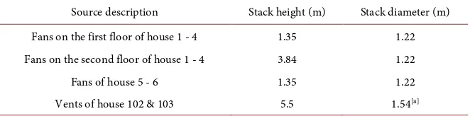
[image:6.595.209.540.627.709.2]

Each fan in the mechanical ventilation systems was considered as an individual horizontal point source. The emissions from side wall curtains of the naturally ventilated houses in spring, summer and fall were considered as area sources; whereas in winter time the 20 ridge vents were considered as 20 capped point sources for houses 102 and 103. The stack heights and stack diameters of point sources were determined based upon the fan diameter and locations (Table 2).

Table 2. Stack heights and stack diameters for point sources.

Source description Stack height (m) Stack diameter (m)

Fans on the first floor of house 1 - 4 1.35 1.22 Fans on the second floor of house 1 - 4 3.84 1.22 Fans of house 5 - 6 1.35 1.22 Vents of house 102 & 103 5.5 1.54[a]

(7)

The stack velocities for horizontal point sources were computed by Equation (3):

2 4

s

V Q D

π

= ⋅ ₍₃₎

where Ds = the stack (fan) diameter

Q = ventilation flow rate of individual fan, m3_s−1

For naturally ventilated houses, the dimensions of the opening of the curtains were the dimension of the area source. For capped point sources, the stack ve-locities were assumed to be the same as wind veve-locities; for area sources, the exit velocities were assumed to be the wind velocities in the direction perpendicular to the side walls.

2.2.3. Plume-Rise Prediction

After completion of all the input files, hourly AERMOD simulations were con-ducted to derive plume rises for the selected data periods specified in Table 3. These hourly simulation followed the processes in the following diagram.

In Figure 4, the RD was compute by comparing the model predicted data

(∆Cp) with the field measurements (∆Cm) using Equation (4):

Table 3. Data periods selected for modeling PM10 dispersion to derive plume rises

through inverse AERMOD method.

Season Year Date period

Fall 2008 October 11-15

Winter 2008 February 4-8

Spring 2009 April 12-13 & April 16-18

Summer 2009 June 18-22

RD: relative difference between model production and field measurement; ∆Cm: measured PM10

concentration at the receptor (downwind minus upwind); ∆Cp: modeled PM10 concentration at the

receptor; ∆h: plume rise.

[image:7.595.208.541.365.671.2]

(8)

( )

% p m

m

C C

RD

C

∆ − ∆

=

∆ (4)

2.3. Data Analysis

After all the hours were run and the ∆hs were determined, seasonal, diurnal and weekly changes of plume rises were then analyzed. As the magnitude of plume rises may be affected by wind direction, wind speed and the temperature differ-ences between ambient and the emission plume flow, these factors were chosen for multiple linear regression analysis. Also, the cloud cover and solar radiation were closely related to the stability class of the ambient environment, and were thus taken into consideration as influencing factors (predictors). Since momen-tum and thermal buoyancy had been the most important factors affecting plume rises, the total volume flow of the exhaust fans was then chosen to represent the momentum of the source. After selecting the possible factors affecting plume rises, a multiple linear regression analysis was conducted to identify the signi-ficance of each selected factor.

3. Results and Discussion

Out of the 435 hourly model runs, 87 valid plume rises were found. The reasons that the rest of the hours were not able to give out a plume rise value are (1) the ∆Cm for that hour was negative, meaning that the measured PM concentration of any possible downwind station was lower than the upwind station; (2) RD> 20%.

3.1. Seasonal Variations of the Plume Rise

Based on the prediction, all plume rises in each season were averaged and com-pared to see if the seasons would affect the magnitude of the plume rises (Table 4). The plume rises of spring and fall were higher than the other two seasons. In winter time, the average plume rise was much lower than other three seasons. This is probably because in winter times, the ventilation rate was not as high as other seasons. In addition, only 15 valid plume rises were obtained for winter time, among which only three hours were from daytime emissions, the plume rises may be affected by diurnal pattern. The average of these 15 plume rises may not well represent the seasonal mean. For summer time, as the thermal buoyan-cy was small due to small temperature differences between emission source and ambient air, the main plume rises were mainly due to the ventilation. However, despite the fact that summer had the highest ventilation rate, the plume rise in summer 2009 was not as much as those in fall 2008 and spring 2009. The plume rises for summer times need to be further investigated.

(9)

[image:9.595.210.540.89.188.2]

DOI: 10.4236/jep.2017.811078 1262 Journal of Environmental Protection Table 4. Mean plume rises by seasons.

Seasons Fall 2008 Winter 2008 Spring 2009 Summer 2009

# of valid plume rises 20 15 33 19 Avg. plume rises (m)* 16.2a _7.9b _16.5a _14.3c

Standard error (m) 11.2 9.5 12.4 10.0 Avg. ventilation (m3_s−1₎ ₁₄₂₁ ₃₂₄ ₁₀₃₃ ₂₂₇₇

Avg. ΔT (˚C) 4.6 18.5 9.0 1.5

[image:9.595.208.541.207.394.2]

*Means with different letters are significant at 0.05.

Figure 5. Diurnal variation of the plume rises.

summer and winter, the ventilation rate is relatively stable (either reached maxi-mum ventilation in summer, or stayed at minimaxi-mum ventilation rate in winter), leading to smaller standard errors for plume rises.

3.2. Diurnal Variation of the Plume Rise

To investigate diurnal variations of the plume rise, the plume rises and the time of a day were sorted together from earlier of the day till the latest ones. The plume rises were then grouped by each two hours from 0:00 to 23:00 and aver-aged within each group. In results, 12 mean plume rises were obtained and shown in Figure 5. As it can be seen, the lowest plume rise appeared at 2:00-3:00 or 18:00-21:00, the highest plume rise appeared at 8:00-9:00. There was no ob-vious diurnal impact on the plume rises by sorting the whole set of data. This was probably because that as the weather changed for different seasons, the ven-tilation varied, thus changing the diurnal patterns. Diurnal results seemed to in-dicate that the time when the peak plume rise appeared may be a matter of other parameters such as ventilation.

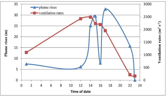
To analyze the response of the plume rises to the house ventilation, both ven-tilation rates and the plume rises for two representative dates were plotted in

Figure 6 & Figure 7. In general, the plume rises responded to the ventilation

(10)

[image:10.595.209.540.62.250.2]

DOI: 10.4236/jep.2017.811078 1263 Journal of Environmental Protection Figure 6. Diurnal variations of the plume rise and ventilation rate on October 11, 2008.

Figure 7. Diurnal variation of the plume rise and ventilation rate on April 16, 2009.

[image:10.595.208.540.278.470.2]

(11)

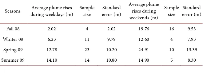
3.3. Comparison of the Plume Rises on Weekday versus Weekends Since the seasonal variation of the plume rises was observed, the comparison of plum rise on weekdays and weekends was conducted within one season. The av-erage plume rises for weekdays and weekends are shown in Table 5.

At a significance level of 0.05, the plume rises during weekends were signifi-cantly higher than those during weekdays (p-value = 0.0019) in Fall. For spring, winter and summer, the difference between the two groups was not significant (p-value = 0.1551, 0.4779 and 0.8763, respectively). Comparison of the plume rises for Fall 2008 and Spring 2009 indicates no significant difference between the weekend plume rises for the two seasons, 19.76 m and 24.91 m; but there was a six times’ difference for the weekday plume rises between these two seasons, 2.02 m and 12.78 m. The fact that Winter 2008 and Spring 2009 had the plume rise ratios of Δhweekends/∆hweekdays in 2.02 and 1.95 implies the plume rises for weekends were about twice as much as the plume rises for weekdays.

For those hours providing valid plume rises, the predicted PM10 concentra-tions by AERMOD for ambient staconcentra-tions were observed to be smaller as the plume rise became larger. This means that if the ambient stations measured greater PM10 concentrations than the true contributions of the farm house emis-sions only, the inverse-AERMOD would produce smaller plume rise. This may explain the observation that the weekday plume rises tend to be smaller than weekend plume rise since there were some traffics around the farm, contributing PM10 to ambient stations. The PM10 contribution of the farm traffics were in-cluded in PM10 measurements at ambient stations and yet not included in emis-sion rate for model simulation.

3.4. Multiple Linear Regression Analysis

[image:11.595.209.539.618.737.2]

To identify the significance of various factors (e.g., wind speed/direction, ambient/ source temperature/RH, solar radiation, ventilation rate) that may affect the plume rise, the linear regression analysis was conducted and results of the analy-sis are listed in Table 6. The p-values of the multiple linear model shows that the wind speed had the strongest relationship with plume rise (p-value = 0.0134). Wind direction, ambient RH and total volume flow had a little relationship with the plume rises (p-value = 0.2285, 0.1709 and 0.2173, respectively). The possible reason for wind speed to be the most important factor would be the fact that the

Table 5. The impact of weekday and weekend on the plume rises.

Seasons Average plume rises during weekdays (m)

Sample size

Standard error (m)

Average plume rises during weekends (m)

Sample size

Standard error (m)

(12)

[image:12.595.209.540.89.270.2]

DOI: 10.4236/jep.2017.811078 1265 Journal of Environmental Protection Table 6. The multiple linear regression modeling results for the simulated plume rises.

Estimate Standard error p-value

Intercept 426.6 192.4 0.0296

Wind direction 0.01474 −0.01214 0.2285

Wind speed 3.283 1.297 0.0134

Ambient temperature 297.2 789.2 0.7075 Source temperature −298.6 789.3 0.7062 Temperature difference 296.5 789.1 0.7081 Ambient RH 0.1239 0.08902 0.1709 Cloud cover 0.2050 0.3617 0.5726 Solar radiation −0.003875 0.01159 0.7391 Total volume flow 0.003245 0.02608 0.2173

exit velocities for naturally ventilated houses were estimated by the wind speeds, which strengthened the relationship between wind speeds and plume rises. It should also be noticed, the ground temperature could also be a possible factor affecting the plume rise of close to ground level emissions. However, no mea-surement of the ground temperature was done during the field data collection.

4. Summary and Conclusions

Based on the 87 predictions of plume rises of AERMOD simulations for the se-lected periods for four seasons, the following findings are obtained:

1) The mean plume rises were 16.2 m (SE = 11.2 m), 7.9 m (SE = 9.5 m), 16.5 m (SE = 12.4 m), 14.3 m (SE = 10.0 m) for fall, winter, spring and summer, re-spectively. More data are needed to support the prediction, especially for winter times.

2) The relationship between time of a day and the plume rises from animal housing systems did not demonstrate consistent diurnal patterns. However, in general, diurnal patterns of the plume rise followed the patterns of the ventila-tion rates.

3) The plume rises during weekends were significantly higher than that during weekends.

4) Wind speed had a very strong positive effect on the plume rises, whereas other parameters (i.e., temperature, RH, ventilation, solar radiation and cloud cover) did not show significant impact (p-value > 0.1) on the magnitude of the plume rises.

Acknowledgements

(13)

was funded by the American Egg Board. Help from Qianfeng Li on field sam-pling is also acknowledged.

References

[1] Guo, L., Maghirang, R.G., Razote, E.B., Trabue, S.L. and McConnell, L.L. (2011) Concentrations of Particulate Matter Emitted from Large Cattle Feedlots in Kansas.

Journal of the Air & Waste Management Association, 61, 1026-1035.

https://doi.org/10.1080/10473289.2011.599282

[2] Donham, K.J., Wing, S., Osterberg, D., Flora, J.L., Hodne, C., Thu, K.M. and Thorne, P.S. (2007) Community Health and Socioeconomic Issues Surrounding Concentrated Animal Feeding Operations. Environmental Health Perspectives, 115, 317-320. https://doi.org/10.1289/ehp.8836

[3] Li, Q-F., Wang-Li, L., Shah, S.B., Jayanty, R.K.M. and Bloomfield, P. (2011) Fine Particulate Matter in a High-Rise Layer House and Its Vicinity. Transaction of the

ASABE, 54, 2299-2310. https://doi.org/10.13031/2013.40649

[4] Li, Q.-F., Wang-Li, L., Walker, J.T., Shah, S.B., Bloomfield, P. and Jayanty, R.K.M. (2012) Particulate Matter in the Vicinity of an Egg Production Facility: Concentra-tions, Statistical Distributions and Upwind and Downwind Comparison.

Transac-tion of the ASABE, 55, 1965-1973. https://doi.org/10.13031/2013.42359

[5] Li, Q-F., Wang-Li, L., Wang, K., Chai, L., Cortus, E.L., Kilic, I., Bogan, B.W., Ni, J-Q. and Heber, A.J. (2013a) National Air Emissions Monitoring Study’s Southeast Layer Site: Part II. Particulate Matter. Transaction of the ASABE, 56, 1173-1184. [6] Li, Q.-F., Wang-Li, L., Jayanty, R.K.M., Shah, S.B. and Bloomfield, P. (2013)

Am-monia Concentrations and Modeling Inorganic Particulate Matter in the Vicinity of an Egg Production Facility. Journal of Environmental Science and Pollutant

Re-search, 21, 4675-4685. https://doi.org/10.1007/s11356-013-2417-z

[7] Wang-Li, L., Li, Q. and Byfield, G.E. (2013) Identifications of Bioaerosols Released from an Egg Production Facility in Southeast U.S. Journal of Environmental

Engi-neering Science, 30, 2-10. https://doi.org/10.1089/ees.2011.0517

[8] Hu, D., Wang-Li, L., Simmons, O.D., Classen, J.J. and Osborne, J.A. (2015) Spati-otemporal Variations of Bioaerosols in the Vicinity of an Animal Feeding Operation Facility in the U.S. Journal of Environmental Protection, 6, 614-627.

https://doi.org/10.4236/jep.2015.66056

[9] Purdy, C.W., Clark, R.N. and Straus, D.C. (2007) Analysis of Aerosolized Particu-lates of Feedyards Located in the Southern High Plains of Texas. Aerosol Science

and Technology, 41, 497-509. https://doi.org/10.1080/02786820701225838

[10] NRC (2003) Air Emissions from Animal Feeding Operations: Current Knowledge, Future Needs. The National Academies Press, Washington DC.

[11] EPA (2004) Ohio’s Largest Egg Producer Agrees to Dramatic Air Pollution Reduc-tions from Three Giant Facilities. Environmental Protection Agency.

http://yosemite.epa.gov/opa/admpress.nsf/b1ab9f485b098972852562e7004dc686/50 8199b8068c24a585256e43007e1230!OpenDocument

[12] EPA (2005) Air Quality Compliance Agreement for Animal Feeding Operations. https://www.epa.gov/afos-air/national-air-emissions-monitoring-study#afo-compli ance-agreement

(14)

DOI: 10.4236/jep.2017.811078 1267 Journal of Environmental Protection https://doi.org/10.13031/2013.24094

[14] Hoff, S.J., Bundy, D.S. and Harmon, J.D. (2008) Modeling Receptor Odor Exposure from Swine Production Sources using CAM. Applied Engineering in Agriculture, 24, 821.https://doi.org/10.13031/2013.25369

[15] Vieira de Melo, A.M., Santos, J.M., Mavroidis, I. and Reis Junior, N.C. (2012) Mod-eling of Odour Dispersion around a Pig farm Building Complex Using AERMOD and CALPUFF. Comparison with Wind Tunnel Results. Building Environment, 56, 8-20.

[16] Ritter, W.F. and Rao Chitikela, S. (2007) Modeling Ammonia and Odor Emissions from Livestock and Poultry Facilities: A Review. World Environmental and Water Resources Congress 2007: Restoring Our Natural Habitat.

https://doi.org/10.1061/40927(243)147

[17] Potter, R.A. (2014) Understanding, Characterizing and Modeling Ammonia Dis-persion near CAFOs. M.S. Thesis, Department of Marine, Earth and Atmospheric Sciences, North Carolina State University, Raleigh.

[18] Zhu, J., Jacobson, L.D., Schmidt, D.R. and Nicolai, R. (2000) Evaluation of INPUFF-2 Model for Predicting Downwind Odors from Animal Production Facili-ties. Applied Engineering in Agriculture, 16, 159-164.

https://doi.org/10.13031/2013.5068

[19] Sarr, J.H., Goïta, K. and Desmarais, C. (2010) Analysis of Air Pollution from Swine Production by using Air Dispersion Model and GIS in Quebec. Journal of

Envi-ronmental Quality, 39, 1975-1983.https://doi.org/10.2134/jeq2009.0199

[20] Bonifacio, H.F., Maghirang, R.G., Auvermann, B.W., Razote, E.B., Murphy, J.P. and Harner III, J.P. (2012) Particulate Matter Emission Rates from Beef Cattle Feedlots in Kansas-Reverse Dispersion Modeling. Journal of the Air & Waste Management

Association, 62, 350-361.https://doi.org/10.1080/10473289.2011.651557

[21] Bonifacio, H.F., Maghirang, R.G., Razote, E.B., Trabue, S.L. and Prueger, J.H. (2013) Comparison of AERMOD and WindTrax Dispersion Models in Determining PM10

Emission Rates from a Beef Cattle Feedlot. Journal of the Air & Waste Management

Association, 63, 545-556.https://doi.org/10.1080/10962247.2013.768311

[22] O’Shaughnessy, P.T. and Altmaier, R. (2011) Use of AERMOD to Determine a Hy-drogen Sulfide Emission Factor for Swine Operations by Inverse Modeling.

At-mospheric Environment, 45, 4617-4625.

[23] Flesch, T.K., Wilson, J.D., Harper, L.A. and Crenna, B.P. (2005) Estimating Gas Emissions from a Farm with an Inverse-Dispersion Technique. Atmospheric

Envi-ronment, 39, 4863-4874.

[24] Flesch, T.K., Wilson, J.D., Harper, L.A., Todd, R.W. and Cole, N.A. (2007) Deter-mining Ammonia Emissions from a Cattle Feedlot with an Inverse Dispersion Technique. Agricultural and Forest Meteorology, 144, 139-155.

[25] Flesch, T.K., Harper, L.A., Powell, J.M. and Wilson, J.D. (2009) Inverse-Dispersion Calculation of Ammonia Emissions from Wisconsin Dairy Farms. Transactions of

the ASABE, 52, 253-265.https://doi.org/10.13031/2013.25946

[26] Jahne, M., Rogers, S., Lopez, K., Kim, S., Grimberg, S. and Holsen, T. (2013) Inverse Dispersion Modeling of Bioaerosol Emissions from Manure Application Sites.

ASABE Annual International Meeting, Kansas City, 21-24 July 2013, Paper No.

131594700.

(15)

DOI: 10.4236/jep.2017.811078 1268 Journal of Environmental Protection [28] Turner, D.B. (1994) Workbook of Atmospheric Dispersion Estimates: An

Introduc-tion to Dispersion Modeling. 2nd EdiIntroduc-tion, Lewis Publishers.

[29] Yadigaroglu, G. and Munera, H.A. (1987) Transport of Pollutants—Summary Re-view of Physical Dispersion Models. Nuclear Technology, 77, 125-149.

https://doi.org/10.13182/NT87-A33979

[30] Crane, G., Panofsky, H. and Zeman, O. (1977) A Model for Dispersion from Area Sources in Convective Turbulence. Atmospheric Environment,11, 893-900. [31] Carney, P.G. and Doddt, V.A. (1989) Comparison between Predicted and Measured

Values for the Dispersion of Malodors from Slurry. Journal of Agricultural

Engi-neering Research,44, 67-76.

[32] Briggs, G.A. (1969) Mathematical Analysis of Chimney Plume Rise and Dispersion: Optimum Formulas for Buoyant Plume Rise. Philosophical Transactions of the

Royal Society of London,265, 197-203.https://doi.org/10.1098/rsta.1969.0048

[33] Cooper, C.D. and Alley, F.C. (2002) Air Pollution Control: A Design Approach. Waveland Press, Prospect Heights.

[34] Weber, A.H. (1976) Atmospheric Dispersion Parameters in Gaussian Modeling. EPA, Washington DC, EPA-600/4-76-030A.

[35] Bennett, M., Sutton, S. and Gardiner, D.R.C. (1991) Measurement of Wind Speed and Plume Rise with a Rapid-Scanning LIDAR. Atmospheric Environment,26A, 1675-1688.

[36] Bennett, M., Sutton, S. and Gardiner, D.R.C. (1992) An Analysis of LIDAR Mea-surement of Buoyant Plume Rise and Dispersion at Five Power Stations.

Atmos-pheric Environment,26A, 3249-3263.

[37] Contini, D. and Robins, A. (2001) Water Tank Measurements of Buoyant Plume Rise and Structure in Neutral Crossflows. Atmospheric Environment, 35, 6105-6115.

[38] Michioka, T., Sato, A., Kanzaki, T. and Sada, K. (2007) Wind Tunnel Experiment for Predicting a Visible Plume Region from a Wet Cooling Tower. Journal of Wind

Engineering and Industrial Aerodynamics, 96, 741-754.

[39] Hanna, S.R., Briggs, G.A. and Chang, J.C. (1997) Lift-Off of Ground-Based Buoyant Plumes. Journal of Hazardous Material, 59, 123-130.

[40] Meroney, R.N. (1979) Lift Off of Buoyant Gas Initially on the Ground. Journal of

Industrial Aerodynamics,5, 1-11.

[41] Briggs, G.A., Britter, R.E., Hanna, S.R., Havens, J.A., Robins, A.G. and Snyder, W.H. (2001) Dense Gas Vertical Dilution over Rough Surfaces: Results of Wind Tunnel Studies. Atmospheric Environment, 35, 2265-2284.

[42] Pasquill, F. (1961) The Estimation of the Dispersion of Windborne Material.

Mete-orology Magazine, 90, 33-40.

[43] Briggs, G.A. (1971) Plume Rise: A Recent Critical Review. Nuclear Safety, 12, 15-24. [44] Briggs, G.A. (1984) Plume Rise and Buoyance Effects. In: Randerson, D., Ed.,

At-mospheric Science and Power Production, U.S. Department of Energy, 327-366.

[45] Calder, K.L. (1977) Multiple-Source Models of Urban Air Pollution—Their General Structure. Atmospheric Environment,11, 403-414.

[46] Pasquill, F. (1971) Atmospheric Diffusion of Pollution. Quarterly Journal of the

Royal Meteorological Society, 97, 369-395.https://doi.org/10.1002/qj.49709741402

(16)

DOI: 10.4236/jep.2017.811078 1269 Journal of Environmental Protection [48] EPA (2003) AERMOD: Latest Features and Evaluation Results. EPA-454/R-03-003.

http://www.epa.gov/ttn/scram/7thconf/aermod/aermod_mep.pdf

[49] Weil, J.C., Corio, L.A. and Brower, R.P. (1997) A PDF Dispersion Model for Buoyant Plumes in the Convective Boundary Layer. Journal of Applied Meteorology

and Climatology, 36, 982-1003.

https://doi.org/10.1175/1520-0450(1997)036<0982:APDMFB>2.0.CO;2

[50] Weil, J.C. (1985) Updating Applied Diffusion Models. Journal of Applied

Meteor-ology and ClimatMeteor-ology, 24, 1111-1130.

https://doi.org/10.1175/1520-0450(1985)024<1111:UADM>2.0.CO;2

[51] Wang, L., Li, Q.-F., Wang, K., Bogan, B.W., Ni, J.-Q., Cortus, E.L. and Heber, A.J. (2013) National Air Emissions Monitoring Study’s Southeast Layer Site: Part I. Site Characteristics and Monitoring Methodology. Transaction of the ASABE, 56, 1157-1171.