Dufour Effects on Unsteady Hydromagnetic Radiative Fluid Flow past a Vertical Plate through Porous Medium

Dufour Effects on Unsteady Hydromagnetic

Radiative Fluid Flow past a Vertical

Plate through Porous

Medium

Jagdish Prakash1*, Avula Golla Vijaya Kumar2, Desu Bhanumathi3, Sibyala Vijaya Kumar Varma3

1_{Department of Mathematics, University of Botswana, Gaborone, Botswana} 2_{Department of Mathematics, Sree Vidyanikethan Engineering College}

(Autonomous), Tirupati, India

3_{Department of Mathematics, S.V. University, Tirupati, India}

Email: *_{prakashj@mopipi.ub.bw, agvijaykumar1729@gmail.com,}

svijayakumarvarma@yahoo.co.in

Received July 23,2012; revised September 1, 2012; accepted September 9, 2012

ABSTRACT

The objective of the present study is to investigate diffusion-thermo (Dufour effect) and radiation effects on unsteady MHD free convection flow past an impulsively started infinite vertical plate with variable temperature and uniform mass diffusion in the presence of transverse applied magnetic field through porous medium. At time t > 0, the plate is given an impulsive motion with constant velocity in the vertical upward direction against to the gravitational field. At the same time the plate temperature is raised linearly with time t and the level of concentration near the plate is raised to . A magnetic field of uniform strength is applied normal to the direction to the flow. The dimen- sionless governing equations are solved in closed form by Laplace-transform technique. The effect of flow parameters on velocity, temperature, concentration, the rate of heat transfer and the rate of mass transfer are shown through graphs.

0 u

w

C B₀

Keywords: MHD; Heat and Mass Transfer; Diffusion-Thermo (Dufour Number); Vertical Plate; Porous Medium

1. Introduction

In nature, there exist flows which are caused not only by the temperature differences but also the concentration differences. These mass transfer differences do affect the rate of heat transfer. In industries, many transport proc- esses exist in which heat and mass transfer takes place simultaneously as a result of combined buoyancy effect in the presence of thermal radiation. Hence, radiative heat and mass transfer play an important role in manu- facturing industries for the design of fins, steel rolling, nuclear power plants, gas turbines and various propulsion device for aircraft, missiles, satellites, combustion and furnace design, materials processing, energy utilization, temperature measurements, remote sensing for astron- omy and space exploration, food processing and cryo- genic engineering, as well as numerous agricultural, health and military applications. If the temperature of

surrounding fluid is rather high, radiation effects play an important role and this situation does exist in space tech-nology. In such cases, one has to take into account the combined effect of thermal radiation and mass diffu- sion.

Boundary layer flow on moving horizontal surfaces was studied by Sakiadis [1]. The effects of transversely applied magnetic field on the flow of an electrically conducting fluid past an impulsively started isothermal vertical plate were studied by Soundalgekar et al. [2]. MHD effects on impulsively started vertical infinite plate with variable temperature in the presence of transverse applied magnetic field were studied by Soundalgekar et al. [3]. The dimensionless governing equations were solved using Laplace transform technique. Kumari and Nath [4] studied the development of the asymmetric flow of a viscous electrically conducting fluid in the forward stagnation point of a two-dimensional body and over a stretching surface with an applied magnetic field. The

governing equations were solved using Laplace trans- form technique.

England and Emery [5] studied the thermal radiation effects of an optically thin gray gas bounded by a sta- tionary vertical plate. Soundalgekar and Takhar [6] con- sidered the radiation free convection flow of an optically thin gray gas past a semi-infinite vertical plate. Radiation effects on mixed convection along isothermal vertical plate were studied by Hossain and Takhar [7]. In all above studies, the stationary vertical plate is considered. Raptis and Perdikis [8] studied the effects of thermal radiation and free convection flow past a moving vertical plate. The governing equations were solved analytically. Das et al. [9] analyzed radiation effects on flow past an impulsively started infinite isothermal vertical plate. The governing equations were solved by the Laplace trans- form technique. Muthucumaraswamy et al. [10] and Ra- jesh and Varma [11] studied radiation and mass transfer effects on exponentially accelerated isothermal vertical plate. Recently, Kumar and Varma [12] studied thermal radiation and mass transfer effects on MHD flow past an impulsively started exponentially accelerated vertical plate with variable temperature and mass diffusion.

Free convection flows that occurs in nature and in en- gineering practice is very large and has been extensively considered by many authors. When heat and mass trans- fer occurs simultaneously between the fluxes the driving potentials are more intricate in nature. An energy flux is generated not only by temperature gradients but by composition gradients as well. Temperature gradients can also create mass fluxes and this is the Soret or Ther- mal-diffusion effect. Generally, the thermal-diffusion and diffusion-thermo effects of smaller order magnitude than the effects prescribed by Fourier’s or Fick’s laws and are often neglected in heat and mass transfer processes. Due to the importance of thermal-diffusion and diffusion- thermo effects for the fluids with very light molecular weight as well as medium molecular weight many invest- tigators have studied and reported results for these flows and the contributors such as Eckert and Drake [13], Dur- sunkaya and Worek [14], Anghel et al. [15], Postenlnicu [16] are worth mentioning. Alam and Rahman [17] stud- ied the Dufour and soret effects on steady MHD free convective heat and mass transfer flow past a vertical porous plate embedded in a porous medium. Alam et al. [18] investigated the Dufour and Soret effects on un- steady free convection and mass transfer flow past an impulsively started infinite vertical plate embedded in a porous medium under the influence of transverse mag- netic field.

In this paper, it is proposed to study diffusion-thermo and radiation effects on MHD free convection flow past an impulsively started infinite vertical plate with variable temperature through porous medium in the presence of

transverse applied magnetic field. The dimensionless governing equations are solved using Laplace transform technique. And the solutions are expressed in terms of exponential and complementary error functions.

2. Mathematical Formulation

Diffusion-thermo and radiation effects on unsteady MHD free convection of flow of a viscous incompressible, electrically, conducting, radiating fluid past an impul- sively started infinite vertical plate with variable tem- perature and uniform mass diffusion in the presence of transverse applied magnetic field through porous me- dium have been studied. The x-axis is taken along the plate in vertical upward direction and -axis is taken normal to it in the direction of applied transverse mag- netic field. Initially, it is assumed that the plate and sur- rounding fluid are at the same temperature and concen- tration in stationary condition for all the points in entire flow region

y

0

y  . At time , the plate is given an impulsive motion with constant velocity 0. At the same time, the plate temperature is raised linearly with time t and the concentration levels near the plate are raised to w

0 t 

uu

C. A magnetic field of uniform strength ₀ is assumed to be applied normal to the flow. For free convection flow, it is also assumed that,

B

1) The inducedmagnetic field is assumed to be negli- gible as the magnetic Reynolds number of the flow is taken to be very small.

2) The viscous dissipation is neglected in the energy equation.

3) The effects of variation in density

 

4) The fluid considered here is gray, absorbing/emit- ting radiation but a non-scattering medium.

5) Since the flow of the fluid is assumed to be in the direction of xaxis, so the physical quantities are func- tions of the space co-ordinate y and only. t

Then by usual Boussinesq’s approximation, the flow is governed by the following equations.









2 2

0 2 u

g T T g C C

t

u

u u

v

k y

 

 _

 

 



 _{    }

 



 



  

 





(1)

2 2

2 2

m T

r p

s

D K q

T T

c

t y y C y



      C

  

    (2)

2 2

C C

D

t y

 

 _ 

 

  (3)





0

0 : 0, , , for all

0 : , , at 0

0, , as

w w

t u T T C C y

t u u T T T T At C C y

u T T C C y

                              (4) where 2 0 u A v

 The local radiant for the case of an opti-

cally thin gray gas is expressed by



4 r

q

a T T

y     _{ }    





It is assumed that the temperature differences within the flow are sufficiently small and that may be ex-

pressed as a linear function of the temperature. This is obtained by expanding

4

T

4

T in a Taylor series about Tand neglecting the higher order terms, thus we get

4 ₄ 3

T  T_ T 3T_4 (6)

From Equations (5) and (6), Equation (2) reduces to





C a T T T

C C y          _{  }          (7)

On introducing the following non-dimensional quanti- ties

















2 2 3

0 3 2 0 0 2 0 2 , , , , , 16 , , , , , w r w w w

r m c

m T w

s p w

g v T T

t u y u T T C C

u

u t y C G

u v v T T C C u

C g v C C v B v a v T

P G S M R

D

u u

D K C C u k

Du k

c c T T                       2 0 , , ku                                     (8)

We get the following governing equations which are

dimensionless _{0 :}0 : _1,0, _,0, _{1 at}0 for all ,_0,

t u C

t u t C y

0, 0, 0 as .

u c y

y                   (12) 2 2 r m u u

G G C Mu

t  y

 

    

 

u

k (9)

3. Solution of the Problem

2 2 2 1 Pr Pr R Du

t y y

  _

 _  _{ } 

   2

C

(10) The appeared physical parameters are defined in the no- _{menclature. The dimensionless governing equations from} (9) to (11), subject to the boundary conditions (12) are solved by usual Laplace transform technique and the solutions are expressed in terms of exponential and com- plementary error functions.

2 2 1

C C

t Sc y

 _ 

  (11)

 

2 y Sc C y t erfc

t

 

 _

 

The initial and boundary conditions in dimensionless

form are as follows:  (13)

 

 





 









Pr Pr Pr Pr

, exp exp

2 4 2 Pr 2 4 2

Pr

exp exp Pr

2 2 Pr

Pr exp Pr Pr 2 exp 2

t y y Rt t y y Rt

y t y R erfc y R erfc

R t R t

b y R

ct y R c erfc c t

t

y R

y R c erfc c t

t b c  _  _ _  __  _  _                _{ }     _  _  _ _    _{ }    _{ }     _  _  _ _      

 









y Sc y Sc

t y cSc erfc ct y cSc erfc ct

 





















 













, exp exp

2 2 2

exp exp

2 4 2 2 4 2

exp

exp exp

2 2 2

A y y

u y t y M erfc M t y M erfc M t

t t

t y y t y y

E y M erfc M t y M erfc M t

M t M t

et y y

B F y M e erfc M e t y M e erfc

t t  _  _ _  _  _{ }  _  _  _         _  _   _  _  _  _{ }  __  _  _  _            _  _  _{ }   _  _   _      









 





















 

















 





2 2 2

exp

exp exp

2 2 2

Pr

exp exp

2 2 Pr

M e t

ct y y

F G y M c erfc M c t y M c erfc M c t

t t

nt y y

G H y M n erfc M n t y M n erfc M n t

t t

B y Rt

y R erfc y R er

t   _        _  _  _  _    _  _   _   _   _       _  _  _  _    _  _   _   _   _           _  _           

 





 









Pr _exp Pr Pr _exp Pr

2 4 2 Pr 2 4 2 P

Pr Pr

exp exp Pr exp Pr

2 2 Pr 2

y Rt

fc t

t y y Rt t y y Rt

E y R erfc y R erfc

R t R t

F y R y

ct y R c erfc c t y R c erfc c

t t         _            _  _ _   _{ }  _  _  _             _{ }  _    _  _  _ _        _{ }  r Pr R





 









 









exp exp Pr exp Pr

2 2 Pr 2

exp

exp exp

2

2 2 2

t

B F y R y R

et y R e erfc e t y R e erfc e t

t t

ct

y Sc y Sc y Sc

Herfc G y cSc erfc ct y cSc erfc ct

t t t

  _{ }  _{ }   _{  }         _{   }    _  _  _ _   _  _{ }       _{  }            _{ }  _  _  _        





 









2 2 2

G H nt y Sc y Sc

y nSc erfc nt y nSc erfc nt

t t   _          _  _  _  _        (15)

Pr _{, ,}

Pr Pr Pr 1

Du Sc R Gr

b c d

Sc Sc

  

   ,

, , ,

Pr 1 1 1 1

M R Gr M Gm

e l n r

Sc Sc Sc

 

   

   

2 2

1 d r, d , d, bd , r

A B E F H

n e c n

e e

      

 n

4. Nusselt Number

From temperature field, now we study Nusselt number (rate of change of heat transfer) which is given in non- dimensional form as

0 y Nu y        _

  (16) From Equations (14) and (16), we get Nusselt number as follows:

 

 

Pr Pr

exp

Pr π Pr 2 Pr

Pr

exp exp Pr

π Pr Pr

exp

π

Rt t Rt Rt

Nu t Rerf erf

R

Rt R

b ct R c erf

t

Sc

b ct cSc erf ct t     _ _     _{   }

 _{ } _  _ c t_ 

    

 

 

 _  _

 

5. Sherwood Number

From concentration field, now we study Sherwood num- ber (rate of change of mass transfer) which is given in non-dimensional form as

0 y C Sh y _      _

π Sc Sh

t 

6. Results and Discussions

In order to get a clear insight of the physical problem the velocity, temperature, concentration, the rate of heat transfer and the rate of mass transfer have been discussed by assigning numerical values to the parameters like ra- diation parameter (R), magnetic parameter (M), Schmidt parameter (Sc), Prandtl number (Pr), Dufour number (Du), thermal Grashof number (Gr), mass Grashof num- ber (Gm) and time t from Figures 1-13 for the cases of

cooling (Gr > 0, Gm >0) and heating (Gr < 0, Gm < 0) of plate. The heating and cooling takes place by setting up free convection currents due to temperature and concen- tration gradient.

Figure 1 depicts the effect of magnetic field parameter

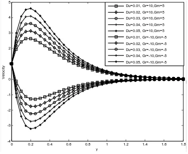
on the fluid velocity and we observed that an increase in magnetic field parameter the velocity decreases in case of cooling of the plate while it increases in case of heat- ing. Figures 2-4 show the effects of R, Du, Gr and Gm on the velocity field u. From these figures, it is observed that the velocity u increases as the radiation parameter R or Dufour number Du or thermal Grashof number Gr or mass Grashof number Gm increases in case of cooling of

the plate and a reverse effect is noticed in the case of heating. The velocity profiles for different values of Schmidt number are shown in Figure 5. From this it is

seen that the velocity decreases with increasing values of Schmidt number in the case of cooling of the plate but increases in the case of heating of the plate. Figure 6

reveals the velocity variation with time t for the cases of both cooling and heating. From this we observed that the velocity increases as time t increases for the case of cooling and the trend is just reversed for the case of heating of the plate. The effect of permeability parameter k on the velocity field is shown in Figure 7. It is seen

from this figure that the velocity increases with increase of permeability parameter k in both cases of cooling and heating of the plate.

The influence of various flow parameters on the fluid temperature are illustrated in Figures 8-10. Figure 8

depicts that the effects of the Dufour number on the fluid temperature. It can be clear seen from this figure that the diffusion thermal effects slightly affect the fluid tem- perature. As the values of Dufour number increase, the fluid temperature is also increases. The effect of thermal radiation R on the temperature field is illustrated in Fig- ure 9. It is obvious that the radiation parameter restricts

the fluid temperature. Therefore, using radiation we can control the fluid temperature. In Figure 10, we depict the

0 0.5 1 1.5 2 2.

-0.2 0 0.2 0.4 0.6 0.8 1 1.2 1.4

y

Ve

lo

c

it

y

M=5, Gr=10,Gm=5 M=6, Gr=10,Gm=5 M=7, Gr=10,Gm=5 M=8, Gr=10,Gm=5 M=9, Gr=10,Gm=5 M=5, Gr=-10,Gm=-5 M=6, Gr=-10,Gm=-5 M=7, Gr=-10,Gm=-5 M=8, Gr=-10,Gm=-5 M=9, Gr=-10,Gm=-5

0 0.5 1 1.5 2 2.5

-0.2 0 0.2 0.4 0.6 0.8 1 1.2 1.4

y

Ve

lo

c

it

y

M=5, Gr=10,Gm=5 M=6, Gr=10,Gm=5 M=7, Gr=10,Gm=5 M=8, Gr=10,Gm=5 M=9, Gr=10,Gm=5 M=5, Gr=-10,Gm=-5 M=6, Gr=-10,Gm=-5 M=7, Gr=-10,Gm=-5 M=8, Gr=-10,Gm=-5 M=9, Gr=-10,Gm=-5

0 0.2 0.4 0.6 0.8 1 1.2 1.4 1.6 1.8 2 -1

-0.5 0 0.5 1 1.5 2

y

Ve

lo

c

it

y

R=4, Gr=10,Gm=5 R=6, Gr=10,Gm=5 R=8, Gr=10,Gm=5 R=8.5,Gr=-10,Gm=-5 R=8.9,Gr=-10,Gm=-5 R=4, Gr=-10, Gm=-5 R=6, Gr=-10, Gm=-5 R=8, Gr=-10, Gm=-5 R=8.5,Gr=-10,Gm=-5 R=8.9,Gr=-10,Gm=-5

0 0.2 0.4 0.6 0.8 1 1.2 1.4 1.6 1.8 2

-1 -0.5 0 0.5 1 1.5 2

y

Ve

lo

c

it

y

R=4, Gr=10,Gm=5 R=6, Gr=10,Gm=5 R=8, Gr=10,Gm=5 R=8.5,Gr=-10,Gm=-5 R=8.9,Gr=-10,Gm=-5 R=4, Gr=-10, Gm=-5 R=6, Gr=-10, Gm=-5 R=8, Gr=-10, Gm=-5 R=8.5,Gr=-10,Gm=-5 R=8.9,Gr=-10,Gm=-5

Figure 2. Velocity profiles when Sc = 2.01, Pr = 0.71, M = 3, k = 5, Du = 0.03 & t = 0.4.

0 0.2 0.4 0.6 0.8 1 1.2 1.4 1.6 1.8

-4 -3 -2 -1 0 1 2 3 4 5

y

Ve

lo

c

ity

Du=0.01, Gr=10,Gm=5 Du=0.02, Gr=10,Gm=5 Du=0.03, Gr=10,Gm=5 Du=0.04, Gr=10,Gm=5 Du=0.05, Gr=10,Gm=5 Du=0.01, Gr=-10,Gm=-5 Du=0.02, Gr=-10,Gm=-5 Du=0.03, Gr=-10,Gm=-5 Du=0.04, Gr=-10,Gm=-5 Du=0.05, Gr=-10,Gm=-5

5

0 0.2 0.4 0.6 0.8 1 1.2 1.4 1.6 1.8

-4 -3 -2 -1 0 1 2 3 4

Du=0.01, Gr=10,Gm=5 Du=0.02, Gr=10,Gm=5 Du=0.03, Gr=10,Gm=5 Du=0.04, Gr=10,Gm=5 Du=0.05, Gr=10,Gm=5 Du=0.01, Gr=-10,Gm=-5 Du=0.02, Gr=-10,Gm=-5 Du=0.03, Gr=-10,Gm=-5 Du=0.04, Gr=-10,Gm=-5 Du=0.05, Gr=-10,Gm=-5

y

Ve

lo

c

it

y

0 0.5 1 1.5 2 2.5 -0.2

0 0.2 0.4 0.6 0.8 1 1.2

y

Ve

lo

c

it

y

Gr=10, Gm=5 Gr=15, Gm=5 Gr=10, Gm=10 Gr=-10,Gm=-5 Gr=-15,Gm=-5 Gr=-10,Gm=-10

0 0.5 1 1.5 2 2.5

-0.2 0 0.2 0.4 0.6 0.8 1 1.2

y

Ve

lo

c

it

y

Gr=10, Gm=5 Gr=15, Gm=5 Gr=10, Gm=10 Gr=-10,Gm=-5 Gr=-15,Gm=-5 Gr=-10,Gm=-10

Figure 4. Velocity profiles when M = 3, Pr = 0.71, Sc = 2.01, R = 10, k = 5, Du = 0.03 & t = 0.4.

0 0.2 0.4 0.6 0.8 1 1.2 1.4 1.6

-3 -2 -1 0 1 2 3 4

y

Ve

lo

c

it

y

Sc=2, Gr=10,Gm=5 Sc=4, Gr=10,Gm=5 Sc=6, Gr=10,Gm=5 Sc=8, Gr=10,Gm=5 Sc=2, Gr=-10,Gm=-5 Sc=4, Gr=-10,Gm=-5 Sc=6, Gr=-10,Gm=-5 Sc=8, Gr=-10,Gm=-5

4

0 0.2 0.4 0.6 0.8 1 1.2 1.4 1.6

-3 -2 -1 0 1 2 3

Sc=2, Gr=10,Gm=5 Sc=4, Gr=10,Gm=5 Sc=6, Gr=10,Gm=5

Sc=8, Gr=10,Gm=5 Sc=2, Gr=-10,Gm=-5

Sc=4, Gr=-10,Gm=-5

Sc=6, Gr=-10,Gm=-5 Sc=8, Gr=-10,Gm=-5

y

Ve

lo

c

ity

0 0.5 1 1.5 2 2.5 3 -0.6

-0.4 -0.2 0 0.2 0.4 0.6 0.8 1 1.2 1.4

y

Ve

lo

c

ity

t=0.2, Gr=10,Gm=5 t=0.4, Gr=10,Gm=5 t=0.6, Gr=10,Gm=5 t=0.8, Gr=10, Gm=5 t=0.2, Gr=-10,Gm=-5 t=0.4, Gr=-10,Gm=-5 t=0.6, Gr=-10,Gm=-5 t=0.8, Gr=-10,Gm=-5

0 0.5 1 1.5 2 2.5 3

-0.6 -0.4 -0.2 0 0.2 0.4 0.6 0.8 1 1.2 1.4

y

Ve

lo

c

ity

t=0.2, Gr=10,Gm=5 t=0.4, Gr=10,Gm=5 t=0.6, Gr=10,Gm=5 t=0.8, Gr=10, Gm=5 t=0.2, Gr=-10,Gm=-5 t=0.4, Gr=-10,Gm=-5 t=0.6, Gr=-10,Gm=-5 t=0.8, Gr=-10,Gm=-5

Figure 6. Velocity profiles when Sc = 2.01, M = 3, Pr = 0.71, R = 10, k = 5, Du = 0.03.

0 0.5 1 1.5 2 2.5

-0.2 0 0.2 0.4 0.6 0.8 1 1.2

y

Ve

lo

c

ity

k=0.5, Gr=10,Gm=5 k=10, Gr=10,Gm=5 k=0.5, Gr=-10,Gm=-5 k=10, Gr=-10,Gm=-5

1.2

1

0 0.5 1 1.5 2 2.5

-0.2 0 0.2 0.4 0.6 0.8

y

Ve

lo

c

it

y

k=0.5, Gr=10,Gm=5

k=10, Gr=10,Gm=5

k=0.5, Gr=-10,Gm=-5

k=10, Gr=-10,Gm=-5

0 0.5 1 1.5 2 2.5 3 3.5 4 0

0.2 0.4 0.6 0.8 1 1.2 1.4

y

T

e

m

perat

ur

e

Du=2.0 Du=5.0 Du=8.0

1.4

0 0.5 1 1.5 2 2.5 3 3.5 4

0 0.2 0.4 0.6 0.8 1 1.2

Du=2.0 Du=5.0 Du=8.0

y

T

em

per

at

ur

e

Figure 8. Temperature profiles when R = 4, Pr = 0.71 & Sc = 2.01.

0 0.2 0.4 0.6 0.8 1 1.2 1.4 1.6

0 0.05 0.1 0.15 0.2 0.25 0.3 0.35 0.4 0.45

y

T

em

per

at

ur

e

R=4, t=0.4 R=6, t=0.4 R=8, t=0.4 R=10,t=0.4

0.45

0.4

0 0.2 0.4 0.6 0.8 1 1.2 1.4 1.6

0 0.05 0.1 0.15 0.2 0.25 0.3

0.35 R=4, t=0.4

R=6, t=0.4

R=8, t=0.4

R=10,t=0.4

y

T

em

p

er

at

ur

e

0 0.2 0.4 0.6 0.8 1 1.2 1.4 1.6 1.8 2 0

0.05 0.1 0.15 0.2 0.25 0.3 0.35 0.4

y

T

e

m

perat

ur

e

Pr=0.1, t=0.2 Pr=0.71,t=0.2 Pr=0.1, t=0.4 Pr=0.71,t=0.4

0 0.2 0.4 0.6 0.8 1 1.2 1.4 1.6 1.8 2

0 0.05 0.1 0.15 0.2 0.25 0.3 0.35 0.4

y

T

em

per

at

ure

Pr=0.1, t=0.2 Pr=0.71,t=0.2 Pr=0.1, t=0.4 Pr=0.71,t=0.4

Figure 10. Temperature profiles when R = 4, Du = 0.03 & Sc = 2.01.

0 0.5 1 1.5 2 2.5 3 3.5 4

0 0.1 0.2 0.3 0.4 0.5 0.6 0.7 0.8 0.9 1

y

C

on

c

ent

rat

ion

Sc=0.22, t=0.4 Sc=0.60, t=0.4 Sc=0.78, t=0.4 Sc=0.96, t=0.4 Sc=0.22, t=0.2 Sc=0.60, t=0.2 Sc=0.78, t=0.2 Sc=0.96, t=0.2

0 0.5 1 1.5 2 2.5 3 3.5 4

0 0.1 0.2 0.3 0.4 0.5 0.6 0.7 0.8 0.9 1

y

C

onc

e

nt

rat

ion

Sc=0.22, t=0.4

Sc=0.60, t=0.4

Sc=0.78, t=0.4

Sc=0.96, t=0.4

Sc=0.22, t=0.2

Sc=0.60, t=0.2

Sc=0.78, t=0.2

Sc=0.96, t=0.2

0.3 0.4 0.5 0.6 0.7 0.8 0.9 1 1.1 1.2 -0.5

0 0.5 1 1.5 2 2.5 3 3.5 4

Time

N

us

s

el

t num

ber

Pr=0.1, R=4, Sc=2.01, Du=0.03 Pr=0.71,R=4, Sc=2.01, Du=0.03 Pr=0.71,R=10,Sc=2.01, Du=0.03 Pr=0.71,R=4, Sc=2.01, Du=2.0

0.3 0.4 0.5 0.6 0.7 0.8 0.9 1 1.1 1.2

-0.5 0 0.5 1 1.5 2 2.5 3 3.5 4

Time

N

u

sse

lt

n

u

m

b

e

r

Pr=0.1, R=4, Sc=2.01, Du=0.03

Pr=0.71,R=4, Sc=2.01, Du=0.03

Pr=0.71,R=10,Sc=2.01, Du=0.03

Pr=0.71,R=4, Sc=2.01, Du=2.0

Figure 12. Nusselt number.

0.5 1 1.5 2 2.5 3

0 0.2 0.4 0.6 0.8 1 1.2 1.4 1.6 1.8

Ti

S

h

erw

ood num

ber

Sc=0.22 Sc=0.60 Sc=0.78 Sc=0.96

0.5 1 1.5 2 2.5 3

0 0.2 0.4 0.6 0.8 1 1.2 1.4 1.6 1.8

Time

S

her

w

o

od n

um

b

er

Sc=0.22 Sc=0.60 Sc=0.78 Sc=0.96

effects of Prandtl number Pr on the temperature field. It

REFERENCES

[1] B. C. Sakiadis vior on Continuous

is observed that an increase in the Prandtl number leads to decrease in the fluid temperature. It is due to the fact that thermal conductivity of the fluid decreases with in- creasing Pr, resulting a decrease in thermal boundary layer thickness.

The concentration profiles for different values of Schmidt number (Sc) and time t are presented in Figure 11. From this figure it is seen that the concentration de-

creases with increase in Sc while it increases with time t.

Figure 12 reveals the rate of heat transfer coefficient in

terms of Nusselt number for different values of radiation parameter R, Prandtl number Pr and Dufour number Dr respectively. It is observed that Nusselt number increases with increasing values of R or Pr but decreases as Du increases. Finally, from Figure 13 it is seen that Sher-

wood number increases with increase of Sc.

, “Boundary Layer Beha

Solid Surfaces: II. Boundary Layer on a Continuous Solid Flat Surfaces,” AIChE Journal, Vol. 7, No. 2, 1961, pp. 221-225. doi:10.1002/aic.690070211

[2] V. M. Soundalgekar, S. K. Gupta and N. S. Birajdar, “Ef- fects of Mass Transfer and Free Convection Currents on MHD Stokes Problem for a Vertical Plate,” Nuclear En- gineering and Design, Vol. 53, No. 3, 1979, pp. 339-346. [3] V. M. Soundalgekar, M. R. Patil and M. D. Jahagirdar,

“MHD Stokes Problem for a Vertical Plate with Variable Temperature,” Nuclear Engineering and Design, Vol. 64, No. 1, 1981, pp. 39-42.

doi:10.1016/0029-5493(81)90030-3

[4] M. Kumari and G. Nath, “Development of Two Dimen-sional Boundary Layer with an Applied Magnetic Field Due to an Impulsive Motion,” Indian Journal of Pure and Applied Mathematics, Vol. 30, No. 7, 1999, pp. 695-708.

[5] W. G. England and A. F. Emery, “Thermal Radiation Effects on the Laminar Free Convection Boundary Layer of an Absorbing Gas,” Journal of Heat Transfer, Vol. 91,

No. 1, 1969, pp. 37-44. doi:10.1115/1.3580116

[6] V. M. Soundalgekar and H. S. Takhar, “Radiation Effects

nd H. S. Takhar, “Radiation Effec on Free Convection Flow past a Semi-Infinite Vertical Plate,” Modeling, Measurement and Control, Vol. 51,

1993, pp. 31-40.

[7] M. A. Hossain a t on

Mixed Convection along a Vertical Plate with Uniform Surface Temperature,” Heat and Mass Transfer, Vol. 31,

No. 4, 1996, pp. 243-248. doi:10.1007/BF02328616

[8] A. Raptis and C. Perdikis, “Radiation and Free

K. Deka and V. M. Soundalgekar,

“Radia-my, K. E. Sathappan, and R.

Natara-and S. V. K. Varma, “Radiation Natara-and Mass

, “Thermal

Ra-d R. M. Drake, “Analysis of Heat anRa-d

Thermo tion Flow past a Moving Plate,” International Journal of Applied Mechanics and Engineering, Vol. 4, No. 4, 1999, pp. 817-821.

[9] U. N. Das, R.

tion Effects on Flow past an Impulsively Started Vertical Infinite Plate,” Journal of Theoretical Mechanics, Vol. 1,

1996, pp. 111-115. [10] R. Muthucumaraswa

jan, “Mass Transfer Effects on Exponentially Accelerated Isothermal Vertical Plate,” International Journal of Ap-plied Mathematics and Mechanics, Vol. 4, No. 6, 2004,

pp. 19-25. [11] V. Rajesh

Transfer Effects on MHD Free Convection Flow past an Exponentially Accelerated Vertical Plate with Variable Temperature,” ARPN Journal of Engineering and Applied Sciences, Vol. 4, No. 6, 2009, pp. 20-26.

[12] A. G. Vijaya Kumar and S. V. K. Varma

diation and Mass Transfer Effects on MHD Flow past an Impulsively Started Exponentially Accelerated Vertical Plate with Variable Temperature and Mass Diffusion,”

Far East Journal of Applied Mathematics, Vol. 55, No. 2 2011, pp. 93-115.

[13] E. R. G. Eckert an

Mass Transfer,” McGraw-Hill, New York, 1972. [14] Z. Dursunkaya and W. M. Worek,

“Diffusion-and Thermal-Diffusion Effects in Transient “Diffusion-and Steady Natural Convection from Vertical Surface, International Journal of Heat Mass Transfer, Vol. 35, No. 8, 1992, pp.

2060-2065. doi:10.1016/0017-9310(92)90208-A

[15] M. Anghel, H. S. Takhar and I. Pop, “Dufour and Soret

ield on Heat and

M. A. Smad, “Dufour

ur and Soret Ef-Effects on Free Convection Boundary Layer over a Ver-tical Surface Embedded in a Porous Medium,” Mathe-matics, Vol. 11, No. 4, 2000, pp. 11-21.

[16] A. Postelnicu, “Influence of a Magnetic F

Mass Transfer by Natural Convection from Vertical Sur-faces in Porous Media Considering Soret and Dofour Ef-fects,” International Journal of Hear and Mass Transfer, 47, No. 6-7, 2004, pp. 1467-1472.

[17] M. S. Alam, M. M. Rahman and

and Soret Effects on Unsteady MHD Free Convection and Mass Transfer Flow past a Vertical Porous Plate in a Po-rous Medium,” Nonlinear Analysis: Modelling and Con-trol, Vol. 11, No. 3, 2005, pp. 217-226.

[18] M. S. Alam and M. M. Rahman, “Dufo

Nomenclature

a B

Absorption coefficient 0

C

External magnetic field Species concentration

w C C

 Concentration of the plate

 Concentration of the fluid far away from the plate

C Dimensionless concentration

p

C Specific heat at constant pressure

s

C Concentration susceptibility g Acceleration due to gravity

r G G

Thermal Grashof number

m Mass Grashof number M Magnetic field parameter Nu Nusselt number

r P q

Prandtl number

r D

Radiative heat flux in the y-direction

m R

Coefficient of mass diffusivity Radiative parameter

c S T

Schmidt number

Temperature of the fluid near the plate

w T T

Temperature of the plate 

t

Temperature of the fluid far away from the plate Time

t Dimensionless time

u Velocity of the fluid in the x-direction 0

u u

Velocity of the plate Dimensionless velocity

y Co-ordinate axis normal to the plate

y Dimensionless co-ordinate axis normal to the plate

Greek Symbols

 Thermal conductivity of the fluid

 Thermal diffusivity

 Volumetric coefficient of thermal expansion

 _{Volumetric coefficient of expansion with}

con-centration

 Coefficient of viscosity

 Kinematic viscosity

 Density of the fluid

 Electric conductivity

 Dimensionless temperature erf Error function

erfc Complementary error function

Subscripts

w Conditions on the wall