RAMANATH, RAJEEV. Interpolation Methods for the Bayer Color Array (under the guidance of Dr. Wesley E. Snyder)
Digital still color cameras working on single CCD-based systems have a mosa-icked mask of color filters on the sensors. The Bayer array configuration for the fil-ters is popularly used. This requires that the data be interpolated to recover all the scene information. Many existing interpolation (demosaicking) algorithms that can reconstruct the scene use modifications of the bilinear interpolation method, intro-ducing a variety of artifacts in the images. These algorithms have been investi-gated. A new method for restoring these color images using an optimization method known as Mean Field Annealing is introduced using a variety of image prior models. Their performance relative to existing demosaicking methods is included.
He was born and brought up for the first few years in a place called Gorakhpur. His family later relocated to Madras (now known as Chennai) where he had his high school education.
In 1998, he earned a Bachelors of Engineering degree from Birla Institute of Technology and Science, Pilani, India, majoring in Electrical Engineering. He has since moved to Raleigh, NC, to pursue “higher” education.
Dedication
Although merely mentioning names in here will by no means satisfy my need to thank all those people involved with the work in this document, I am bound to mention a few here. I would like to thank my advisor, Dr. Wesley Snyder for all the support and guidance pro-vided, not to mention his innate ability to discuss problems on the basis of scientific intel-lect.
Special gratitude goes to Dr. H. J. Trussell for his valuable insight. Also my gratitude goes to Dr. Jack Holm (HP Labs) for all the help with the data gathered; to Dr. Toshi Hori (Pulnix America Inc.) for all the help with providing us with data and a camera to perform experiments. Also, I wish to thank Dr. Y.F. Yoo (Texas Instruments), who had been very helpful in providing calibration information about the cameras.
Dr. James Adams (Eastman Kodak Company) deserves a lot of credit for his insight and advice during the course of this project, which he offered ever so willingly.
Many thanks to Dr. Griff Bilbro, Dr. Paul Hemler and Dr. Richard Kuehn for their encour-agement and direction and timely guidance.
It would be unfair if I did not thank my parents, Ramanath and Meera and my sister, Ramya, for having stood by me in every decision I have made; Sumathi, for being there for me and understanding my every idiosyncrasy; my friends, who helped me review my work, en-courage me and help me sort things out; thankyou.
LIST OF TABLES . . . viii
LIST OF FIGURES . . . ix
Chapter 1 Introduction. . . . 1
Color Filter Arrays . . . .2
Demosaicking . . . .4
Outline . . . .6
Chapter 2 Color Fundamentals . . . .7
Introduction . . . .7
Retinal Receptors of the Human Eye. . . .8
Color Models . . . .11
Color Matching Functions . . . 12
RGB Color Model . . . 12
HSV Color Model . . . 17
CIE-XYZ Color Model . . . 19
Color Differences. . . 24
CIE-L*a*b* Color Model . . . 27
ISO RGB Color Model . . . 29
sRGB Color Model (for displays) . . . 34
Caveat (Interpolating in Color Space) . . . .35
Chapter 3 Image Model . . . .37
Introduction . . . .37
Linear Model . . . .37
a-priori imaging constraints . . . .41
Blur . . . 42
Noise . . . 43
Median-based Interpolation . . . .53
Gradient Based Interpolation . . . .56
Adaptive Color Plan Interpolation . . . .59
Comparison of Interpolation Methods . . . .63
Type I Test Images . . . 64
Type II Images . . . 69
Type III Images . . . 70
RGB Images. . . 73
Results . . . .79
Chapter 5 MFA Restoration Methods . . . .86
Introduction . . . .86
Reconstruction processes . . . .86
Mean Field Annealing . . . .87
Noise Term . . . 92
Prior Term . . . 93
Choice of parameters . . . 98
Chapter 6 Demosaicking using Mean Field Annealing . . . .103
Introduction . . . .103
Independent Restoration (MFA-RGB). . . .103
Independently Piecewise Uniform . . . 104
Independently Piecewise Linear . . . 104
Vector MFA (VMFA). . . .105
VMFA - Noise Term . . . 105
VMFA - Prior Term . . . 106
CFA Sampling . . . .110 Synthetic Images . . . 112 Chapter 8 Results . . . .116 Introduction . . . .116 Synthetic Images . . . .117 Real-world Images . . . .130 Measures . . . .146 Chapter 9 Improvements . . . .149 Introduction . . . .149
Constant-Hue based Interpolation . . . .150
Median-Based Interpolation. . . .152
Vector median based interpolations . . . .154
Chapter 10 Conclusion and Future Work . . . .155
References . . . .157
Appendix A Gamma Correction Explained . . . .163
Table 4.1 metric 81
Table 4.2 metric (x10-3) 81
Table 5.1 Parameter list for MFA 98
Table 7.1 metric for subpixel Gaussian blurred images 114
Table 7.4 metric (x10-3) for subpixel Gaussian blurred images 114 Table 8.1 Error Metrics for piecewise-constant restored images 125 Table 8.2 Error Metrics for piecewise-linear restored images 130 Table 8.3 Number of floating point operations required for a 256x256
image 147 ∆Eab * ∆ERGB ∆Eab * ∆ERGB
LIST OF FIGURES
Figure 1.1 The four possible arrangements of the Bayer Array Sensors 2 Figure 1.2 Yamanaka Color Filter Array. Chrominance samples are
out of phase on each scanline
3 Figure 1.3 Illustration of mosaicking artifacts (a) Original reference
image (b) a small portion from that image (c) result of lin-ear interpolation
5
Figure 2.1 Color components of light, based on nanometers. Note: names do not define wavelength regions, but are for the main regions of the spectrum. The visible region of the spectrum is from about 400 to 700 nm.
8
Figure 2.2 The scotopic and photopic sensitivities of the Human eye. Notice the region where the sensitivity is highest in each case.
9
Figure 2.3 Color sensitivity of the human eye. 10
Figure 2.4 Principle of trichromatic color matching by additive mixing of lights. R, G, B are sources of red, green and blue light, the intensities of whose can be adjusted. C is the target color the observer needs to match by changing the intensi-ties of R, G, B.
13
Figure 2.5 The color matching functions of the CIE RGB standard rep-resented in terms of the stimulus provided by the three wavelengths mentioned in the text
15
Figure 2.6 The RGB Color Cube 17
Figure 2.7 The HSV Color hexcone 19
Figure 2.8 The CIE-XYZ color matching curves. 21
Figure 2.9 The chromaticity diagram viewed in the CIE XYZ model Notice that the hues are not evenly spaced about the perim-eter of this “Horse-shoe” plot.
orientation.
Figure 2.11 Subjectively equal color steps on the chromaticity diagram. Each line segment represents a color difference about three times greater than that just noticeable distance for a 2ofield.
26
Figure 2.12 ISO RGB Color Matching Functions 31
Figure 2.13 OECF for a typical DSC [52] 33
Figure 2.14 Illustration of results of interpolating in different color spaces (a) original image (b) RGB interpolation (c) HSV interpolation
36
Figure 3.1 Image formation model in a digital camera system 38
Figure 4.1 Sample Bayer Pattern 46
Figure 4.2 Illustration of fringe or zipper effect resulting from the lin-ear interpolation process (a) Original image (only 2 colors) (b) subsampled Bayer image (c) result of linear interpola-tion. Notice color fringe in locations 5 and 6
47
Figure 4.3
a) RGB image b) Green Channel c) Green minus Red
(d)Green minus Blue 52
Figure 4.4 Illustration of Freeman’s interpolation method for a two channel system (a) Original image (b) subsampled Bayer image (c) result of linear interpolation (d) Green minus Red (e) median filtered result of the difference image (f) recon-structed image
54
Figure 4.5 Sample Bayer Neighborhood Ai = Chrominance, Gi = Luminance
59
Figure 4.6 Bayer Array Neighborhood 62
Type I Test Images, a) Test Image1 has vertical bars with decreasing thicknesses(16 pixels down to 1 pixel) b) Test
Figure 4.8
(a)Linear (b)Cok (c)Freeman (d)Laroche-Prescott
(e)Hamilton-Adams interpolations on Test Image1. Note: Images are not the same size. Image has been cropped to
hide edge effects 66
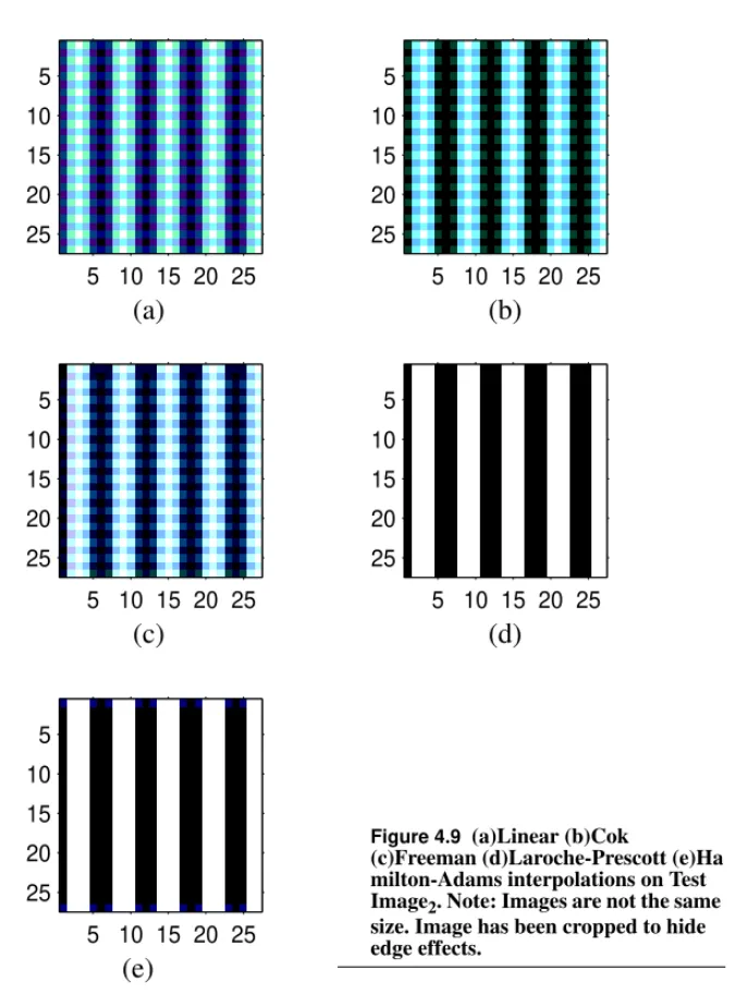
Figure 4.9 (a)Linear (b)Cok (c)Freeman (d)Laroche-Prescott (e)Ha milton-Adams interpolations on Test Image2. Note: Images are not the same size. Image has been cropped to hide edge effects
68
Figure 4.10 Type II Test Images, a) has horizontal bars with decreasing thicknesses(16 pixels down to 1 pixel) b) Constant width (3 pixels
69
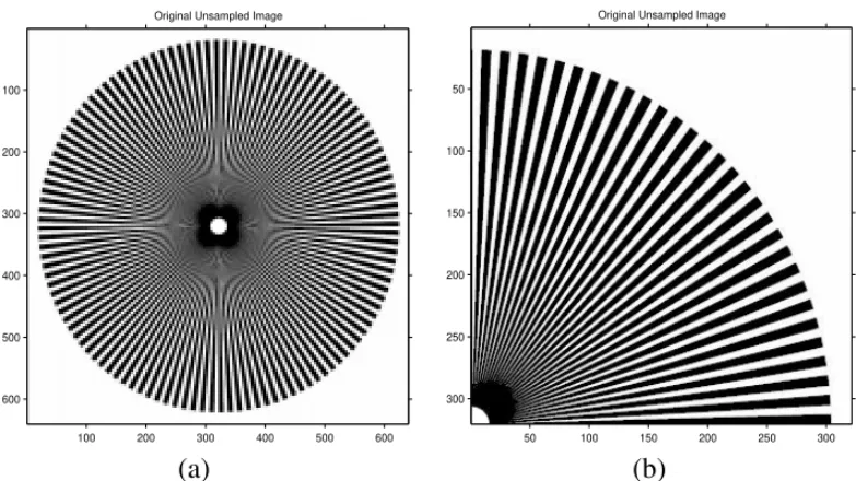
Figure 4.11
Type III Test Image, a) Full-size Starburst Image b) Upper
right quadrant, used in tests 70
Figure 4.12 (a)Linear (b)Cok (c)Freeman (d)Laroche-Prescott (e)Hamilton-Adams interpolations on Starburst Image. Note: Images are not the same size. Image has been cropped to hide edge effects.
72
Figure 4.13 (a) Full-resolution macaw Image (b) ROI about the green macaws’ eye (c) ROI about the red macaws’ eye
74 Figure 4.14 (a)Linear (b)Cok (c)Freeman (d)Laroche-Prescott
(e)Hamilton-Adams interpolations on macaw Image show-ing ROI about the green macaw’s eye.
75
Figure 4.15 (a)Linear (b)Cok (c)Freeman (d)Laroche-Prescott
(e)Hamilton-Adams interpolations on macaw image show-ing ROI about the red macaw’s eye
76
Figure 4.16 (a)Full-resolution girl Image (b) ROI about the balloon rib-bon (c) ROI about the girl’s mouth
77 Figure 4.17 (a)Linear (b)Cok (c)Freeman (d)Laroche-Prescott
(e)Hamilton-Adams interpolations on girl image showing ROI about the balloon ribbon
Figure 5.1 Illustration of blur estimation process (a) sample image showing CFA pattern (b) samples in red channel along the horizontal axis
101
Figure 6.1 Flow-chart showing the proposed restoration process 109 Figure 7.1 Illustration of the “missing-pixel” artifact (a) Original CFA
image (b) Result after Linear Interpolation
111 Figure 7.2 Type I Test Image, a) Test Image2 used earlier (b) Test
Image2 after a 2x2 boxcar blur (c) TestImage2 after a sub-pixel blur of variance unity and subsampled accord-ingly.(bars of constant width - 3 pixels)
113
Figure 8.1 Piecewise-constant synthetic images (a) Test Image1 (b) Test Image2 (c) Test Image3 (d) Test Image4
118 Figure 8.2 MFA Restored Test Image1 (a) result of de-mosaicking (b)
MFA-RGB (c) VMFA (d) MFA-HSV restoration
119 Figure 8.3 MFA Restored Test Image2 (a) result of de-mosaicking (b)
MFA-RGB (c) VMFA (d) MFA-HSV restoration
121 Figure 8.4 MFA Restored Test Image3 (a) result of de-mosaicking (b)
MFA-RGB (c) VMFA (d) MFA-HSV restoration
122 Figure 8.5 Regions of interest in the starburst image (a) ROI1(b) ROI2 123 Figure 8.6 MFA Restored ROI1 of the starburst image (a) result of
de-mosaicking (b) MFA-RGB (c) VMFA (d) MFA-HSV resto-ration
124
Figure 8.7 MFA Restored ROI2 of the Starburst image (a) result of de-mosaicking (b) MFA-RGB (c) VMFA (d) MFA-HSV resto-ration
124
Figure 8.8 Piecewise-linear synthetic images (a) Test Image5 (wedge) (b) Test Image6(color wedges)
Figure 8.10 ROI in the color wedges image 128 Figure 8.11 MFA Restored ROI of the color-wedges image (a) result of
de-mosaicking (b) MFA-RGB (c) VMFA (d) MFA-HSV restoration
129
Figure 8.12 CFA “resolution chart” image 131
Figure 8.13 Regions of interest in the resolution chart image (a) ROI1 (b) ROI2
132 Figure 8.14 MFA Restored ROI1 of the Resolution chart image (a)
result of de-mosaicking (b) MFA-RGB (c) VMFA (d) MFA-HSV restoration
133
Figure 8.15 MFA Restored ROI2of the resolution chart image (a) result of de-mosaicking (b) MFA-RGB (c) VMFA (d) MFA-HSV restoration
134
Figure 8.16 CFA “matisse” image 135
Figure 8.17 Regions of interest in the matisse image (a) ROI1 (b) ROI2 136 Figure 8.18 MFA Restored ROI1 of the matisse image (a) result of
de-mosaicking (b) MFA-RGB (c) VMFA (d) MFA-HSV resto-ration
137
Figure 8.19 MFA Restored ROI2of the resolution chart image (a) result of de-mosaicking (b) MFA-RGB (c) VMFA (d) MFA-HSV restoration
138
Figure 8.20 CFA “books” image 139
Figure 8.21 Region of interest in the books image 140
Figure 8.22 MFA Restored ROI1 of the matisse image (a) result of de-mosaicking (b) MFA-RGB (c) VMFA (d) MFA-HSV resto-ration
141
Figure 8.23 CFA “car” image 142
Figure 8.24 Region of interest in the car image 143
Figure 8.27 Error rates in the restoration process vs. step count 148 Figure 9.1 Example spectral sensitivities of a digital color camera [52] 150 Figure 9.2 Improvement on Cok’s algorithm (a) original RGB image
(b) result of Cok’s algorithm (c) result of using the new def-inition of hue
152
Figure 9.3 Modification of Freeman’s algorithm (a) original RGB image (b) result of Freeman’s algorithm (c) result of using the mean instead of the median
153
Figure A.1 Illustration of gamma correction for displays (a) Original Input to display (b) as seen on a monitor with gamma of 2.5 (c) gamma-corrected input (d) as seen after gamma correc-tion
164
Figure A.2 Image profiles and gamma correction curves for the images used earlier (a) Original Input to display (b) as seen on a monitor with gamma of 2.5 (c) gamma-corrected input (d) as seen after gamma correction
164
Figure A.3 Illustration showing how gamma correction affects hue (a) actual color as seen on a display with a gamma of 2.5 (b) color simulated with a gamma correction of 1.0
Chapter 1
Introduction
Digital Color Cameras sample the spectrum of visible light using three or more fil-ters. Each location on the CCD (photo-site) captures one sample of the color spec-trum. This gives us a “mosaic” of samples. The process of recovering the original image is referred to as demosaicking. The choice of the sensitivities of the CCD elements is critical.
To reconstruct a color image, we need to sample luminance and chrominance information. Since the Human Visual System (HVS) is less sensitive to degrada-tions in the chrominance information than those in the luminance information [29], the chrominance channels are often sub-sampled by a larger magnitude than the luminance channels. In other words, since there needs to be a sub-sampling in the scene information, the chrominance channels may be sampled at a rate much lower than the luminance channel.
It shall be shown later that the spectral sensitivity of the HVS to luminance is sim-ilar to the spectral power distribution of the green channel. Hence, green sensors replace the luminance channel. Red and blue sensors replace the chrominance channels. We can now construct a color filter to perform the sampling of the color spectrum.
1.1 Color Filter Arrays
The Bayer Array [9] is one of the many realizations of color filter arrays possible. It has a mosaic of red, green and blue optical filters which can be described by a simple 2x2 arrangements as shown in Figure 1.1.
R G G B B G G R G R B G G B R G
Figure 1.1 The four possible arrangements of the Bayer Array Sensors (phase shifted)
The arrangements describe the upper left corner of the sensor array. The rest of the sensor array can be determined by repeating this pattern both horizontally and ver-tically in both the spatial dimensions.
Other implementations of a color-sampling grid have been incorporated in com-mercial cameras, also using the principle that the luminance channel needs to be sampled more than the chrominance channels. For instance, the pattern shown in Figure 1.2, developed by Yamanaka [55] is widely used in digital cameras pro-duced by Sony Corporation. This can be repeated in a similar fashion with a hori-zontal alignment to the green data.
There are many more arrangements of these filters published, but not all been implemented, for reasons of complexity and costs. These include arrays obtained
R G G G R R G G G B B B B G G G B B G G G R R R G R B R G G B R B G G G G B R B G G R B R G G G
Figure 1.2 Yamanaka Color Filter Array. Chrominance samples are out of phase on each scan-line
developed in hexagonal grids forms by Fujifilm Inc. etc. (implemented recently with good success [30]).
In this dissertation, however, we shall look at Bayer Color Arrays.
1.2 Demosaicking
The “mosaic” of colors needs to be “undone” to recover three color planes in order to obtain a full color reproduction of the scene information. This process is referred to as demosaicking. There are a variety of methods available for this inter-polation process, which shall be discussed.
In this dissertation, we restore images obtained from the mosaicking process in order to reduce the artifacts observed.
Included in Figure 1.3 are results obtained from demosaicking using linear inter-polation (details discussed in Chapter 4), highlighting the need for a restoration step. The original image [1] is shown in Figure 1.3a, a region of interest of which is extracted in Figure 1.3b. Linear interpolation gives rise to artifacts in the image
Demosaicking
as shown in Figure 1.3c. These images are included here just to give the reader an idea of the problem at hand.
(a)
(b)
1.3 Outline
In Chapter 2, a review of color fundamentals is presented, which forms a basis for the rest of the dissertation. Chapter 3 describes a generic camera imaging model. Chapter 4 introduces the available demosaicking methods and compares their per-formances on test images, highlighting their advantages and disadvantages. Chap-ter 5 reviews generic restoration techniques in image processing, with concentration on the Mean Field Annealing (MFA) process. In Chapter 6, the sug-gested method for restoration is introduced, describing the fundamentals of vector based MFA. The experimental approach and the caveats involved have been described in Chapter 7. Results obtained are given in Chapter 8. Chapter 9 briefly describes possible improvements to existing demosaicking algorithms. The disser-tation and its results and findings have been concluded in Chapter 10.
Chapter 2
Color Fundamentals
2.1 Introduction
The understanding of color lays its foundations on the experiments conducted by Sir Isaac Newton in 1666 [36], [42]. Until then, opinions on the nature of color and their interactions were not well defined. Newton made a small hole in an otherwise dark room; through this hole, the direct rays of the sun could shine and form an image of the sun’s disc on the opposite wall of the room, much like a pin-hole cam-era. Then, taking a prism of glass and placing it close to the hole, he observed that the light spread out into what he called a spectrum, colored red, orange, yellow, green, blue, indigo, and violet along its length. The natural conclusion was that white light was not simply a homogenous entity, but was composed of a mixture of colors of the spectrum.
used as a rough guide; each color gradually changes into the other color and there are no definite boundaries. Also to be noted is that the appearance of a color is dependent upon viewing conditions (foreground color, background color, lighting, etc.). and varies from one viewer to another.
2.2 Retinal Receptors of the Human Eye
In general, the retina has two kinds of receptors, rods and cones.
The primary function of the rods is to provide monochromatic vision under low
Ultra
violet
V
iolet
Blue Green Yello
w
Orange Red Infrared
300 400 500 600 700 800 Wavelength, nm
380 450 490 560 590 630 780
Figure 2.1 Color components of light, based on nanometers. Note: names do not define wavelength regions, but are for the main regions of the spectrum. The visible region of the spectrum is from about 400 to 700 nm.
Retinal Receptors of the Human Eye
The rods have a photosensitive pigment called rhodopsin. This pigment absorbs light most strongly in the blue-green region of the spectrum. As a result, the spec-tral sensitivity of the rods is as shown in Figure 2.21. This part of human vision is referred to as scotopic vision.
400 450 500 550 600 650 700 0 0.2 0.4 0.6 0.8 1 Efficiency Wavelength (nm) Photopic Vision Scotopic Vision
Figure 2.2 The scotopic and photopic
The function of the cones in the retina is to provide color vision at normal levels of vision (usually, several candela per square meter. This results in photopic vision.
The cones are primarily of three types, namely the based on their indepen-dent sensitivities to different wavelengths of light.
β γ ρ, , 400 450 500 550 600 650 700 0 0.2 0.4 0.6 0.8 1 1.2 1.4 β cones γ cones ρ cones
Color Models
As can be seen by comparing Figure 2.3 and Figure 2.1, the correspond to the sensitivities in approximately the blue-violet, green and yellow-orange regions of the spectrum respectively. It is interesting to note the substantial spectral overlap of the and cones.
2.3 Color Models
The essential principles of three color-measurements were first introduced and pre-sented as axioms by Grassman as long ago as 1853 has made the acceptance of trichromatic stimuli, axiomatic [42].
Color measuring devices have sensors with frequency spread over the spectrum. This spectrum has a certain wavelength called the dominant frequency. The domi-nant frequency being the one at which the spectral response function of that device has a peak. The whole spectrum can be reconstructed by these spectral response functions by simple linear or non-linear combinations of the available frequencies. Let us look at a few of the different color models used to try and best represent the
β γ ρ, ,
2.3.1 Color Matching Functions
Color vision is basically a function of three variables. These are the three different types of cones. Although the rods provide a fourth spectrally different receptor, there is overwhelming evidence [15] that at some later stage of the visual system, the number of variables is reduced to three. Hence, it is expected that the evalua-tion of perceived color from spectral power data should require the use of three dif-ferent spectral weighting functions.
At levels of illumination that are high enough for color vision to be operating prop-erly, there is evidence that the outputs of the rods is rendered ineffective. At levels where both rods and cones are operating together, color vision must be based on four different spectral sensitivities; but, at these levels color discrimination is not very good.
2.3.2 RGB Color Model
Color Models
used and by W. D. Wright[53] who used three light sources along with test color patches in a set-up as shown below in Figure 2.4. Their results were normalized to three monochromatic light sources (Red-700nm, Green-546.1 nm, and Blue-435.8nm).
This choice of green and blue were made because of the light source being used
-Diffuser Diffuser Aperture Plate G B R C Observer’s eye
Figure 2.4 Principle of trichromatic color matching by additive mixing of lights. R, G, B are sources of red, green and blue light, the intensities of whose can be adjusted. C is the target color the observer needs to match by changing the intensities of R, G, B.
wavelength calibration as hue changes slowly with wavelength at the wavelengths near red [32].
The subject would match a certain color patch on the target by “combining” the three wavelengths and it was observed that it was possible to map the visible color spectrum using the , weighting functions, shown in Figure 2.5. An interesting point to note is the negative values the red weight function takes. This is done not because there is negative light! It is only a convenient way to represent experimental fact that one of the matching stimuli, in this case, red, had to be added to the color being matched instead of to the mixture.
Color Models
These colors are called additive colors because they can be added to produce dif-ferent colors; meaning, if one power unit of one wavelength is matched by
400 450 500 550 600 650 700 −0.1 −0.05 0 0.05 0.1 0.15 0.2 0.25 0.3 0.35 0.4 Wavelength (nm) Sensitivity r(λ) g(λ) b(λ)
Figure 2.5 The color matching functions of the CIE RGB standard represented in terms of the stimulus provided by the three wavelengths mentioned in the text
λ1
,
then the additive mixture of the two lights, and is matched by
.
This means that the color-matching functions of Figure 2.5 can be used as weight-ing functions to determine the amounts of R, G, B needed to match any color, if the amount of power per small-constant-width wavelength interval is known for that color throughout the spectrum.
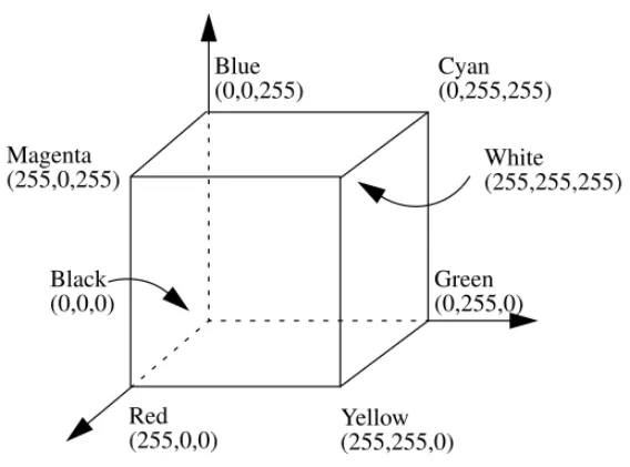
In the R, G, B color model described above, the amounts of R, G and B are referred to as tristimulus values. The RGB color model requires tristimulus values that could be negative. This is not very desirable as a certain display which uses, say electron beams striking on phosphors, would not be able to reproduce this “negative” input, to match the complete color gamut. In general, a display system has stimuli which can vary from 0 to 255. This is represented as an RGB color cube as shown in Figure 2.6. The RGB Color model that is used in color displays,
r2of R+g2of G+b2of B
λ1 λ2
r1+r2
Color Models
use tristimulus values in the range of [0,255]. This model is represented as a color cube shown in Figure 2.6.
2.3.3 HSV Color Model
Color, as perceived by the human eye has three essential characteristics, hue, satu-ration and intensity. Hue represents dominant color as perceived by an observer;
Red Blue Green Black White Cyan Magenta Yellow (255,255,0) (255,0,0) (255,255,255) (0,255,255) (0,0,255) (255,0,255) (0,0,0) (0,255,0)
refers to the relative purity or the amount of white light mixed with a hue. The degree of saturation is inversely proportional to the amount of white light added. Intensityembodies the achromatic notion of brightness (luminance) and is one of the key factors in describing color sensation. It is a subjective descriptor of the amount of energy an observer perceives from a light source. This model was ini-tially designed for artists to input and mix their painting colors on a computer drawing [16], [43]. The HSV Color model is represented as a hexcone as shown in Figure 2.7. The hexcone is of unit height. Hue is measured as the angle from the red axis. When S is zero, the value of H is irrelevant as it is a shade of gray (achro-matic). Any color with V=1 and S=1 is akin to an artist’s “pure” color pigment used at the starting point of mixing colors. Adding white pigment corresponds to decreasing S, without changing V.
The top of the HSV hexcone corresponds to the projection seen by looking along the principal diagonal of the RGB cube from white toward black. Subcubes of the RGB cube correspond to different slices along the V axis of the hexcone. This gives an intuitive correspondence between RGB and HSV color models. RGB to HSV conversion algorithms are included in Appendix B.
Color Models
2.3.4 CIE-XYZ Color Model
To mitigate the problem with the RGB color model of negative stimuli, the CIE (Commision Internatinale de l’Eclairage), a body responsible for international rec-ommendations for photometry and colorimetry devised a new color model which used transformations of the RGB model such that tristimulus values were never
S H 0.0 Red Green Blue V 1.0 Magenta 0o 120o 240o Yellow Cyan White Black
This transformed color space is called the CIE-XYZ color space. The transforma-tion is given by means of the following equatransforma-tions:
(2.1)
The numbers for these set of equations were carefully chosen so that X, Y, Z would always be positive for all colors as is seen in Figure 2.8.
Another advantage of this color model is that the Y component represents lumi-nance of a color. The color matching curves we had for the RGB color model transform to the XYZ color model by Equation 2.1.
X Y Z 0.49 0.31 0.20 0.17697 0.81240 0.01063 0 0.01 0.99 R G B =
Color Models
Notice, in Figure 2.8, the curve spans most of the spectrum. When compared to Figure 2.2, the spectral response of the photopic vision is very close to that of
.
Three new stimuli replace the existing X, Y, Z values, x, y, z (normalized) where,
400 450 500 550 600 650 700 0 0.2 0.4 0.6 0.8 1 1.2 1.4 1.6 1.8 Wavelength (nm) Sensitivity x(λ) y(λ) z(λ)
Figure 2.8 The CIE-XYZ color matching curves1.
y( )λ
(2.3)
(2.4)
A plot of the x, y space is called the chromaticity diagram is shown in Figure 2.9. Colors in the XYZ model are represented as ordered triplets of , where x, y record the chromaticity values while Y gives the luminance.
y Y X+Y +Z ( ) ---= z Z X+Y+Z ( ) ---= x y Y, , ( )
Color Models
In Figure 2.9, the point E, , is the equi-energy stimulus point. Figure 2.9 The chromaticity diagram viewed in the CIE XYZ model Notice that the hues are not evenly spaced about the perimeter of this “Horse-shoe” plot1.
x y z 1
3
2.3.5 Color Differences
In the RGB color model, one could use three colors in the RGB cube, a, b, c which are set apart such that , i.e. the colors have the same Euclidean distance between them, where,
(2.5)
It is observed, however, that this measure is not uniform (constant) over the color space. For instance, colors with the same maybe be perceived as having no resemblance at all or on the other hand they may be perceived as being very simi-lar.
Some of the first controlled experiments on “similar” colors were conducted by MacAdam [36]. Observers were asked to match two color patches in an experi-ment similar to the one described in Figure 2.4 and the error in matching yielded sensitivity ellipses in the chromaticity diagram as shown in Figure 2.10. The ellipses represent differences in chromaticity that are just noticeable.
∆ERGBab = ∆ERGBbc
∆ERGB ((R1–R2)2+(G1–G2)2+(B1–B2)2) 1 2 ---= ∆ERGB
Color Models
As was the case with the RGB model, the CIE XYZ model also suffers from the same problem of perceptual imbalance. This is illustrated in the Figure 2.11.
0 0.1 0.2 0.3 0.4 0.5 0.6 0.7 0.8 0 0.1 0.2 0.3 0.4 0.5 0.6 0.7 0.8 0.9 X Y MacAdam Ellipses
Figure 2.10 The result of pioneering work done by MacAdams, resulting in ellipses that were a marker to the just noticeably different colors. Ellipses are scaled up in size to enhance orientation1.
Notice, in Figure 2.11, the line segments are not all of equal length. In the region near the greens, the line-segments are longer than those near the reds and purples implying non-uniformity (non-constancy) in color differences. Equal length line
Figure 2.11 Subjectively equal color steps on the chromaticity diagram. Each line segment represents a color difference about three times greater than that just noticeable distance for a 2o field.
Color Models
segments throughout the chromaticity diagram would imply uniformity in the color differences (hence, perceptual balance), which is desired in the color model.
2.3.6
CIE-L*a*b* Color Model
From earlier sections, it is concluded that there is a need for a perceptually bal-anced color model that the human visual system can to relate to.
Two of the color models suggested by the CIE which are perceptually balanced and uniform are the CIE-L*u*v* and the CIE-L*a*b* color models. The L*u*v* model is based on the work by MacAdams on the Just Noticeable Differences [36] in color.
These color models are transformations of the XYZ color model.
(2.6) L* 116 Y Yn --- 1 3 ---16 for Y Yn --->0.008856 – 903.3 Y Yn --- for Y Yn ---≤0.008856 =
(2.7)
, (2.8)
where Xn, Yn, Zn are the values of X, Y, Z, for the appropriately chosen reference
white; and where, if any of the ratios , , is equal to or less than 0.008856,
it is replaced in the above formula by
where F is , , , as the case may be.
The color differences in the L*a*b* color model are given by
(2.9) a* 500 X Xn --- 1 3 ---Y Yn --- 1 3 ---– = b* 200 Y Yn --- 1 3 ---Z Zn --- 1 3 ---– = X Xn --- Y Yn --- Z Zn ---7.787F 16 116 ---+ X Xn --- Y Yn --- Z Zn ---∆Eab * (∆L*)2 ∆a* ( )2 (∆b*)2 + + [ ] 1 2 ---=
Color Models
In general differences of about 2.3 or greater are noticeable [37] and those over 10 are so different that comparison is not worthwhile.
In the rest of this dissertation, differences shall be used in conjunction with mean square error, primarily because it is the errors that the human eye can detect - perceptual errors. The mean square error shall be used in conjunction as it is a mathematical measure that most methods use as a cost function.
2.3.7 ISO RGB Color Model
The spectral responses of the color analysis channels of digital still cameras (DSCs) do not, in general, match those of a typical human observer [52], defined by the CIE standard colorimetric observer. Neither do the responses of different DSCs necessarily match each other. There is hence a need to characterize these DSCs with help of color matching functions and illuminants and map them onto a reference color space.
∆Eab
*
∆Eab*
∆Eab
The International Organization for Standardization (ISO), along with experts in the field of digital cameras, is working on a standard for digital cameras to character-ize them using color targets spectral illumination.
The process of transforming from the color space of the camera to a uniform color space has been addressed [42], [49].
The ISO RGB represents an estimate of the scene or original colorimetry. As such, it maintains the relative luminance ratio and the color gamut of the scene or origi-nal.
Color Models
These color matching functions have been derived using the spectral sensitivity of the sensors in digital color cameras; unlike the RGB color matching functions shown in Figure 2.5, which were developed for the human eyes’ spectral sensitivi-ties. 350 400 450 500 550 600 650 700 750 800 850 −0.1 −0.05 0 0.05 0.1 0.15 0.2 0.25 Wavelength (nm) Sensitivity Red Green Blue
DSCs use non-linear, usually logarithmic amplifiers in the conversion from light intensity to voltage output. These values need to be converted into a linear space before they can be transformed into the XYZ (uniform) color space.
The transformation from the logarithmic camera space to the linear space is done by the use of the Opto Electronic Conversion Function (OECF). The OECF for a typical digital still color camera [32] is shown in Figure 2.13 where the horizontal axis denotes the data output of the camera (from the sensors in the camera, which is in the range of [0,255] and vary in a non-linear fashion) and the vertical axis cor-responds to the linear domain of the data captured.
Color Models
For a D65 luminant, the transform matrix is given by
(2.10)
where , , are R, G, B values in after transforming by the OECF.
0 50 100 150 200 250 300 0 500 1000 1500 2000 2500 3000 3500 4000 4500
Camera Digital Level
OECF Data
Figure 2.13 OECF for a typical DSC [52]
X Y Z 0.4124 0.3576 0.1805 0.2126 0.7152 0.0721 0.0193 0.1192 0.9505 RLin GLin BLin =
Once in a linear space, the data can be modified or transformed into the color-gamut of the device being used.
2.3.8 sRGB Color Model (for displays)
To be able to display colors, in the desired colorimetric settings, there is a tendency to display images using the perceptually balanced color models like the CIE-L*a*b*, or the CIE-L*u*v* color models. This is however not practical due to the complexity of the transformations required.
This standard, like the ISO RGB standard is a working standard. It attempts to standardize the color gamut available to commercial PC- and web-based color imaging systems, aiding in precise reproduction of images on different displays.
The three major factors of the sRGB space are the colorimetric RGB definition, the equivalent gamma value (display’s tonal transfer function, see Appendix A for details) of 2.2 and well-defined viewing conditions, along with a number of sec-ondary details.
Caveat (Interpolating in Color Space)
The transformation matrix for a gamma value of 2.2 (standard) and a D50 illumi-nant is given below in Equation 2.11.
(2.11)
where , , are R, G, B values in the sRGB Color Space.
The reader is referred to [32] for further details.
2.4 Caveat (Interpolating in Color Space)
The result of interpolation depends on the color space in which the interpolation is being performed. If the conversion from one color model to another is linear (can be represented as a matrix multiplication, like RGB, YIQ), then the results of lin-ear interpolation in both models will be the same [16]. However, in the case of non-linear transformations (HSV, CIE-L*a*b*, CIE-L*u*v*), the results are not the same as those produced in, say the RGB space. This is illustrated in
RsRGB GsRGB BsRGB 3.2410 –1.5374 –0.4986 0.9692 – 1.8760 0.0416 0.0556 –0.2040 1.0570 X Y Z = RsRGB GsRGB BsRGB
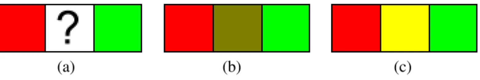
red(255,0,0) and green(0,255,0). Equally weighted linear interpolation in the RGB space results in (128,128,0) - brown. On the other hand, estimating the center pixel from red(0o,1,1) and green(120o,1,1) in the HSV model, results in (60o,1,1) which, in RGB space is (255,255,0) - yellow. This needs to be borne in mind while per-forming operations in linear and non-linear spaces. If the objective is to maintain fixed hue (or saturation) between colors during interpolation, the HSV model may be preferable [16].
(a) (b) (c)
Figure 2.14 Illustration of results of interpolating in different color spaces (a) original image (b) RGB interpolation (c) HSV interpolation
Chapter 3
Image Model
3.1 Introduction
Image models provide a backbone on which algorithms can be designed and implemented. In this chapter we look at the image formation model used in Digital Still Color Cameras (DSC).
3.2 Linear Model
We shall consider the image formation model to be linear in nature [50]. The image formation model in a camera system is based on a continuous-discrete model [41] where the input data (scene) is continuous while the capture device (CCD) is discrete. Figure 3.1 shows such a model.
The input/output relationship for this system is given by
(3.1)
where , a band-limited image obtained from the CCD in the th sensor type, is discrete (with uniformly spaced samples), f, the scene, is continuous and h, the point-spread function (PSF), is continuous. is the spectral sensitivity of the sen-sor with non-zero spectral sensitivity between and . is a discrete space
CCD Array
Scene Camera System
h
f g
Figure 3.1 Image formation model in a digital camera system
gλ i(x y, ) f(ξ η λ, , )h x ξ( – ,y–η,λ)L λ( ) ξd dη λd ∞ – ∞
∫
∞ – ∞∫
λl l λi u∫
+ελi(x y, ) = gλ i λi L λi l λi u x y, ( )Linear Model
about the blur kernel and the noise are discussed in later sections. The form of Equation 3.1 assumes that the PSF is space invariant.
Sampling this equation (without noise considerations) for a discrete approximation [41], we get
(3.2)
The two dimensional image formation models have long used the stacked notation to represent the mathematics involved, especially in image restoration problems [6]. This is also referred to as a lexicographic notation.
Consider a gray-scale F image (only one color channel, say red) of size NxN pix-els. In other words,
(3.3)
where the fi are column vectors of length N each. The resulting lexicographic rep-resentation for F is given by
g x y( , ) f k l( , )h x k( – ,y–l) l=0 N–1
∑
k=0 M–1∑
= F = f1 f2 … fNwhere the superscript T corresponds to a transpose operation. f is now a N2x1 col-umn vector. Generating the blur kernel H, as an N2xN2block Toeplitz matrix [41], we can represent the blurred image formation model as a matrix multiplication operation using
. (3.5)
Introducing signal independent additive noise to the system, we can represent the formed image g, as
(3.6) where is the additive noise of the imaging system. This image is now sampled with the CFA mask in the color channel under consideration. The advantages of using this notation is the ease of use in written form. Also, when the expected val-ues of such terms and their products are transformed into the Fourier domain (especially in restoration processes), the result is easier to handle than what may be expected [41].
g = Hf
g = Hf+ε
a-priori imaging constraints
3.3
a-priori imaging constraints
The assumption of non-negativity must be maintained throughout our models since optical energies inherent in imaging must always be non-negative quantities. Both the measurement and the true image being non-negative imply that the PSF must also be non-negative.
(3.7) (3.8) (3.9) An important assumption that needs to be made is that we have a lossless system, meaning that the energy in the object is preserved in the image; i.e. the lens and other parts of the imaging system do not absorb or generate optical energy. In the continuous-discrete case [6], (3.10) which implies f(ξ η, ) 0≥ g x y( , ) 0≥ h(ξ η, ) 0≥ f(ξ η, ) ξ ηd d ∞ – ∞
∫
∞ – ∞∫
g x y( , ) y=0 M–1∑
x=0 N–1∑
= ∞∫
∞∫
3.3.1 Blur
In this dissertation, we model PSFs introduced due to the optics in the system (out-of-focus blurs). An out-(out-of-focus blur for a circular aperture is represented by an airy disk [33]. The airy disk has a PSF which is given by
(3.12)
However, owing to its ease in implementation and the fact that small out-of-focus blurs may be modeled by a Gaussian PSF, we will the out-of-focus blur using a Gaussian PSF, given by
(3.13)
where is the blur variance and are the mean values describing position of the blur. In our case however, the blur will be centered about the origin, making the mean values zero.
h(ξ η, ) 1 πR2 --- ,((ξ2+η2) R≤ 2) 0 ,else = h(ξ η, ) 1 2πσ --- (ξ ξ– ) 2 η η – ( )2 + 2σ2 ---– exp = σ ξ η,
a-priori imaging constraints
3.3.2 Noise
The noise introduced in the system is modeled as additive zero-mean white Gauss-ian noise, for each channel. This is an approximation to the noise process which is in fact a Poisson process. For the purpose of this document, we approximate the noise process as a signal-independent non-negative Gaussian process. For a small signal variance, this assumption is widely accepted.
The noise samples have a probability distribution given by
(3.14)
To maintain the requirement of Equation 3.8 of non-negativity, the pixel values in the image need to be clipped.
p( )ς 1 2πσ --- ς2 2σ2 ---– exp =
methods in Bayer Arrays
4.1 Introduction
Commercially available Digital Still Color Cameras (DSC), as mentioned in Sec-tion 1.1, are based on a single CCD array and capture color informaSec-tion by using three or more types of color filters, each pixel capturing only one sample of the color spectrum. This mosaic, needs to be populated with information from all the color planes in order to obtain a full resolution true color image. This process is referred to as demosaicking.
To reconstruct the complete color image, interpolation must be performed on the image data. There are a variety of methods available, the simplest being linear interpolation, which, as shall be shown does not maintain edge information well. More complicated methods [14], [17], [24], [22], [34], [35] perform this interpola-tion and attempt to maintain edge detail or limit hue transiinterpola-tions.
Ideal Interpolation
In this chapter, we shall assume that the images are not corrupted by noise. Also, we shall assume that the images do not have a PSF associated with them (or rather, the PSF is an ideal impulse). In Chapter 7 and Chapter 8, we will consider the effects out-of-focus-blurs and noise.
4.2 Ideal Interpolation
Following the sampling theory, the sampling of a continuous image yields infinite repetitions of its continuous spectrum in the Fourier domain, which do not overlap. If this is so, and only then, the original image can be reconstructed perfectly from its discrete samples . The 1- D ideal interpolation is the mul-tiplication with a rect function in the frequency domain and can be realized in the spatial domain by a convolution with the sinc function. The “ideal interpolator” kernel is band-limited and hence is not space limited. This interpolator, hence is not feasible to implement in practice.
4.3 Bilinear Interpolation
f x y( , )
f x y( , ) f m n( , )
At a blue center, we need to estimate the green and red components. Consider pixel 44 at which only B44is measured; we need to determine G44. Given G34, G43, G45, G54, one estimate for G44 is given by
(4.1)
To determine R44, given R33, R35, R53, R55, the estimate for R44 is given by
(4.2)
and at a red center, we would estimate the blue and green accordingly. Performing
R11 G12 R13 G14 R15 G16 G21 B22 G23 B24 G25 B26 R31 G32 R33 G34 R35 G36 G41 B42 G43 B44 G45 B46 R51 G52 R53 G54 R55 G56 G61 B62 G63 B64 G65 B66 R71 G72 R73 G74 R75 G76 R17 R37 R57 R77 G27 G47 G67
Figure 4.1 Sample Bayer Pattern
G44 (G34+G43+G45+G54) 4 ---= R44 (R33+R35+R53+R55) 4 ---=
Bilinear Interpolation
planes for the scene which would give us one possible demosaicked form of the scene. This type of interpolation is a low pass filter process.
The band-limiting nature of this interpolator smoothens edges, which show up in color images as fringes (referred to as the zipper effect [1], [2]). This has been illustrated with two colors channels (for simplicity) in Figure 4.2.
2 1 3 4 5 6 7 8 9 10 11 12 1 2 3 4 5 6 7 8 9 10 11 12 2 1 3 4 5 6 7 8 9 10 11 12 (a) (b) (c)
Figure 4.2 Illustration of fringe or zipper effect resulting from the linear
interpolation process (a) Original image (only 2 colors) (b) subsampled Bayer image (c) result of linear interpolation. Notice color fringe in locations 5 and 6.
4.4 Constant Hue-based Interpolation
This method proposed by Cok [14] and is one of the first few methods used in commercial camera systems. Modifications of this system are still in use. The key objection of pixel artifacts in images that result from bilinear interpolation is abrupt and unnatural hue change. There is a need to maintain the hue of the color such that there are no sudden jumps in hue (but for over edges, say). Chrominance channels correspond to the red and blue channels while the luminance channel is the green channel.
As used herein, the term hue refers to a quantity relating to a value of a color sam-pled at lower resolution to the value of a color samsam-pled at higher resolution. In other words, the hue is defined by [14]. It is to be noted that the term hue
defined above is valid for this method only, also, the hue needs to be “redefined” if the denominator G is zero. By interpolating the hue value and deriving the interpo-lated chrominance values (blue and red) from the interpointerpo-lated hue values, hues are allowed to change only gradually, thereby reducing the appearance of color fringes which would have been obtained by interpolating only the chrominance values.
R G ---- B G ----,
Constant Hue-based Interpolation
Consider an image with constant hue. The values of the luminance (G) and one chrominance component (R, say) at one location (Rij, Gij) and another sample location (Rkl, Gkl) are related as
if (4.3)
in exposure space (be it logarithmic1 or linear).
If Rkl represents the unknown chrominance value, and Rij and Gij represent mea-sured values and Gkl represents the interpolated luminance value, the missing chrominance value Rkl is given by
(4.4)
In an image that does not have uniform hue, as in a normal color image, smoothly changing hues are assured by interpolating the hue values between neighboring chrominance values.
1. Most cameras capture data in a logarithmic exposure space and need to be linearized before the ratios used
Rij Rkl --- Gij Gkl ---= Bij Bkl --- Gij Gkl ---= Rkl Gkl Rij Gij --- =
The green channel however is interpolated first using bi-linear interpolation, to populate the green channel’s checkerboard pattern. After this first pass, the hue is interpolated.
In other words, referring to Figure 4.1,
(4.5)
and similarly for the blue channel
(4.6)
In Equation 4.5 and Equation 4.6, the G values in bold-face are estimated values, after the first pass of interpolation. The extension of the logarithmic exposure space is a straightforward as multiplications become additions and divisions become subtractions in the logarithmic space. There is a caveat however as inter-polations will be performed in the logarithmic space and hence the relations in lin-ear space and exposure space are not identical [14]. Hence in most
implementations the data is first linearized and then interpolated as mentioned
R44 G44 R33 G33 --- R35 G35 --- R53 G53 --- R55 G55 ---+ + + 4 ---⋅ = B33 G33 R22 G22 --- R24 G24 --- R42 G42 --- R44 G44 ---+ + + 4 ---⋅ =
Neighborhood considerations
4.5 Neighborhood considerations
We could possibly get better estimates for the missing pixels by increasing the neighborhood of the pixel, but this increase is expensive in terms of memory con-siderations which is not desirable. There is hence a need to keep the interpolation filter kernel space-limited to a small size and also extract as much information from the neighborhood as possible. The correlation between color signals is often used [1]. For RGB images, cross-correlation between channels has been deter-mined and found to vary between 0.25 and 0.99 with averages of 0.86 for red/ green, 0.79 for red/blue and 0.92 for green/blue cross correlations [46]. One well-known image model is to simply assume that red and blue are perfectly correlated with the green over a small neighborhood. This image model is stated as
(4.7) where refers to the pixel location, R (known) and G (unknown) the red and green pixel values, k is the appropriate bias for the given pixel neighborhood. The same applies at a blue pixel location. Let us illustrate Equation 4.7 with an exam-ple, by considering the green channel of an image and the corresponding Green
Gij = Rij+k
of the regions in the Green minus Red and Green minus Blue images are uniform, especially in regions where there is high spatial detail (near the eyes of the
macaws). 50 100 150 200 250 300 350 50 100 150 200 250 50 100 150 200 250 300 350 50 100 150 200 250 50 100 150 200 250 300 350 50 100 150 200 250 50 100 150 200 250 300 350 50 100 150 200 250
Figure 4.3 a) RGB image b) Green Channel c) Green minus Red (d)Green minus Blue
(a) (b)
Median-based Interpolation
4.6 Median-based Interpolation
This method, proposed by Freeman [17], is a two pass process, the first being a lin-ear interpolation, and the second pass a median filter of the color differences.
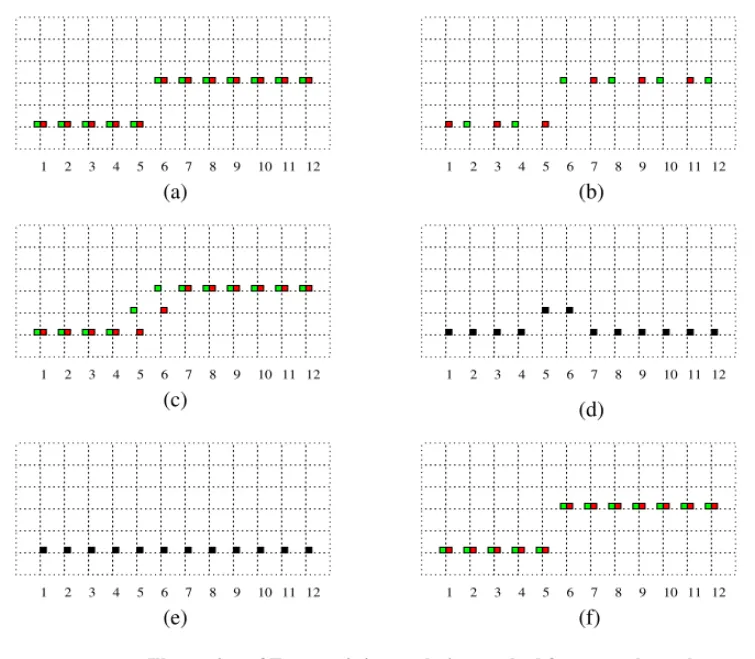
In the first pass, linear interpolation is used to populate each photo-site with all three colors and in the second pass, the difference image, of say, Red minus Green and Blue minus Green is median filtered. This median filtered image is then used in conjunction with the original bayer pattern samples to recover the samples. This method preserves edges very well, as illustrated in Figure 4.4. Only one row of the Bayer array is considered since this process can be extrapolated to the case of the rows containing blue and green pixels. In Figure 4.4, where (a) shows the original image before Bayer subsampling (b); (c) shows the result of linear interpolation. Notice the color fringes introduced between pixels 5 and 6; (d) shows the absolute valued difference image between the two channels; (e) shows the result of median filtering the difference image with a kernel of size 5. Using the result obtained from (e) and the original Bayer image (b), (f) is generated to produce a recon-structed version of the original scene image. The reconstruction of the edge is
This concept can be carried over to three color sensors wherein differences are cal-culated between pairs of colors and the median filter is applied to these differences to generate the final image. In other words, referring to Figure 4.2;
2 1 3 4 5 6 7 8 9 10 11 12 1 2 3 4 5 6 7 8 9 10 11 12 2 1 3 4 5 6 7 8 9 10 11 12 1 2 3 4 5 6 7 8 9 10 11 12 2 1 3 4 5 6 7 8 9 10 11 12 1 2 3 4 5 6 7 8 9 10 11 12 (a) (b) (c) (d) (e) (f)
Figure 4.4 Illustration of Freeman’s interpolation method for a two channel system (a) Original image (b) subsampled Bayer image (c) result of linear interpolation (d) Green minus Red (e) median filtered result of the difference image (f) reconstructed image
ˆ + =
Median-based Interpolation (4.9) where (4.10) (4.11) Similarly, (4.12) (4.13) where (4.14) (4.15) and (4.16) (4.17) where R44 = rˆb+B44 rˆg = median R( i–Gi) i ℵ, ∈ G34 r ˆb = median R( i–Bi) i ℵ, ∈ B44 G33 = gˆr–R33 G44 = gˆb+B44 gˆr = median R( i–Gi) i ℵ, ∈ R33 gˆb = median G( i–Bi) i ℵB, ∈ 44 B33 = bˆr+R33 B34 = bˆg+G34 ( ) i ℵ, ∈
In the above equations, refers to the neighborhood of pixel under consideration. The size of this neighborhood is variable.
We shall consider neighborhoods of a size such that all the algorithms can be com-pared on the same basis. The algorithms described in this chapter have at most 9 pixels under consideration for estimation. In a square neighborhood, this would imply a 3 x 3 window. We shall hence use a 3 x 3 neighborhood for Freeman’s algorithm.
4.7 Gradient Based Interpolation
This method, proposed by Laroche and Prescott [35] and is in use in the Kodak DCS 200 Digital Camera System. It employs a three step process, the first one being the interpolation of the luminance channel (green) and the second and third being bilinear interpolation of the chrominance channels (red and blue).
This method takes advantage of the fact that the human eye is most sensitive to luminance changes. Depending upon the position of an edge, in the green channel, the interpolation is performed accordingly.
Gradient Based Interpolation
Referring back to Figure 4.2, if we need to estimate G44, let
(4.20)
(4.21)
are estimates to the horizontal and vertical second-derivatives respectively, in blue. It is intriguing to note that the classifiers used are second derivatives with the sign inverted and halved in magnitude. Using these second derivatives as classifi-ers, we come up with the following estimates for the missing green pixel value.
(4.22)
(4.23)
(4.24)
Similarly, for estimating G33, let
(4.25) α abs (B42+B46) 2 ---–B44 = β abs (B24+B64) 2 ---–B44 = α β, G44 (G43+G45) 2 --- if(α β< ) = G44 (G34+G54) 2 --- if(α β> ) = G44 (G43+G45+G34+G54) 4 --- ifα β = = α abs (R31+R35) 2 ---–R33 = β (R13+R53)
are estimates to the horizontal and vertical second derivatives in blue, respec-tively. Using these gradients as classifiers, we come up with the following esti-mates for the missing green pixel value.
(4.27)
(4.28)
(4.29)
Once the luminance is determined, the chrominance values are interpolated from the difference of color differences between the color (red and blue) and luminance (green) signals. This is given as follows
(4.30)
(4.31)
(4.32)
Note however, that the green channel has been completely populated before this step. The bold-face entries correspond to estimated values. We get corresponding
α β, G33 (G32+G34) 2 --- if(α β< ) = G33 (G23+G43) 2 --- if(α β> ) = G33 (G32+G34+G23+G43) 4 --- ifα β = = R34 (R33–G33)+(R35–G35) 2 --- G 34 + = R43 (R33–G33)+(R35–G35) 2 --- G 43 + = R44 (R33–G33)+(R35–G35)+(R53–G53)+(R55–G55) 4 --- G 44 + =
Adaptive Color Plan Interpolation
the green component has the advantage of maintaining color information and also using intensity information at pixel locations.
At this point, three complete RGB planes are available for the image.
4.8 Adaptive Color Plan Interpolation
This method is proposed by Hamilton and Adams [22]. It is a modification of the method proposed by Laroche and Prescott [35]. The concept is similar to that of using second derivatives as an estimate for the data; but uses the second derivative in conjunction with the gradient estimate.
Consider the Bayer array neighborhood as shown below in Figure 4.5.
A3 G2 A1 A7 G4 G8 G6 A5
This process also has three runs. The first run populates that luminance (green) channel and the second and third runs populate the chrominance (red and blue) channels.
Gi is a green pixel and Ai is either a red pixel or a blue pixel (All Ai pixels will be the same color for the entire neighborhood).
We now form the following classifiers
(4.33) (4.34) We use the term “classifiers” as these are used to classify a pixel as belonging to a vertical or a horizontal edge. These are not “estimates” of a derivative as they are combinations of the first derivative and the second derivative.
These classifiers are composed of second derivative terms for chromaticity data and gradients for the luminance data. As such, these classifiers sense the high spa-tial frequency information in the pixel neighborhood in the horizontal and vertical directions.
α = abs(–A3+2 A5–A7) abs G+ ( 4–G6)
Adaptive Color Plan Interpolation
Consider, that we need to estimate the green value at the center, i.e. to estimate G5. Depending upon the preferred orientating, the interpolation estimates are deter-mined.
(4.35)
(4.36)
(4.37)
These predictors are composed of arithmetic averages for the green data and appropriately scaled second derivative terms for the chromaticity data. This com-prises the first pass of the interpolation algorithm.
The second pass involves populating the chromaticity channels. Consider the neighborhood as shown below in Figure 4.6.
G5 (G4+G6) 2 --- –A3+2 A5–A7 4 --- + if α β( < ) = G5 (G2+G8) 2 --- –A1+2 A5–A9 4 --- + if α β( > ) = G5 (G2+G4+G6+G8) 4 --- –A1–A3+4 A5–A7–A9 8 --- + if α β = =
Giis a green pixel and Aiis either a red pixel of a blue pixel and Ciis the opposite chromaticity pixel.
(4.38)
(4.39)
The two cases in Equation 4.38 and Equation 4.39 are those when the nearest neighbors to Ai are in the same column and row respectively. To estimate C5, we employ the same method as we did to estimate the luminance channel.
We again, form two classifiers, which “estimate” the gradient in the horizontal and vertical directions.
A1 G2 A3
G4 C5 G6
A7 G8 A9
Figure 4.6 Bayer Array Neighborhood
A2 (A1+A3) 2 --- –G1+2G2–G3 2 --- + = A4 (A1+A7) 2 --- –G1+2G4–G7 2 --- + = α β,
Comparison of Interpolation Methods
(4.41) In Equation 4.40 and Equation 4.41, sense the high frequency information in the pixel neighborhood in the positive and negative diagonal respectively.
(4.42)
(4.43)
(4.44)
These predictors are composed of arithmetic averages for the chromaticity data and appropriately scaled second derivative terms for the green data. Depending upon the preferred orientation of the edge, the predictor is chosen.
We now have the three color planes populated for the Bayer Array data.
4.9 Comparison of Interpolation Methods
The above mentioned methods are a few of those employed in commercial cam-eras today. A few test images, shown in Figure 4.7, Figure 4.10, Figure 4.11, are
β = abs(–G1+2G5–G9) abs A+ ( 1–A9) α β, A5 (A3+A7) 2 --- –G3+2G5–G7 2 --- + if α β( < ) = A5 (A1+A9) 2 --- –G1+2G5–G9 2 --- + if α β( > ) = A5 (A1+A3+A7+A9) 4 --- (–G1–G3+4G5–G7–G9) 4 ---+ if α β = =
these are cases that consider “what-if” cases in the Bayer Array. These particular images were chosen as test images to emphasize the various details that each algo-rithm works on. The images have been broken down into three categories depend-ing upon the dominant edge orientation and the fourth set of images are RGB images.
4.9.1 Type I Test Images
These images have a predominantly horizontal orientation to their gradient direc-tions i.e. their edges are as shown in Figure 4.7
.
10 20 30 40 50 60 10 20 30 40 50 60 10 20 30 5 10 15 20 25 30
Figure 4.7 Type I Test Images, a) Test Image1 has vertical bars with decreasing