Lookup Table Optimization for Sensor Linearization in
Small Embedded Systems
Lars E. Bengtsson
Physics Department, University of Gothenburg, Gothenburg, Sweden Email: [email protected]
Received October 5, 2012; revised November 6, 2012; accepted December 6, 2012
ABSTRACT
This paper treats the problem of designing an optimal size for a lookup table used for sensor linearization. In small em- bedded systems the lookup table must be reduced to a minimum in order to reduce the memory footprint and intermedi- ate table values are estimated by linear interpolation. Since interpolation introduces an estimation uncertainty that in- creases with the sparseness of the lookup table there is a trade-off between lookup table size and estimation precision. This work will present a theory for finding the minimum allowed size of a lookup table that does not affect the overall precision, i.e. the overall precision is determined by the lookup table entries’ precision, not by the interpolation error.
Keywords: Lookup Table; Sensor Linearization; Embedded Systems; Interpolation
1. Introduction
Look-up tables (LUTs) are used in a wide variety of computer and embedded applications; NASA use it to improve the pointing precision of antennas [1], CERN uses LUTs to calibrate the beam energy acquisition sys- tem of the Large Hadron Collider (LHC) [2] and it is one of the most common methods for digital synthesis of ar- bitrary waveforms [3]. It is used extensively in numeric calculations, for example in division algorithms [4], square root algorithms [5] and even for fast evaluation of general functions [6,7]. In Data Acquisition Systems (DAQ) it is used to correct non-linearities and offset errors in Analog-to-Digital Converters (ADCs) [8-10] or to design non-uniform ADCs [11]. This work will focus mainly on LUT applications in Embedded Measurement Systems (EMS); linearizing sensor signal outputs is one of the major applications of LUTs [12-18].
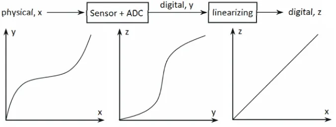
A sensor converts the physical unit (the measurand) into some electrical unit (preferably volt) and the em- bedded measurement system converts the sensor output into a digital value (typically an integer) [19]. The main errors in most measurement systems are related to the transducer’s offset, gain and non-linearities [20], and for that reason the process of sensor linearization is a crucial step in the design of an embedded measurement system [21]. The linearization process must compensate for the non-linear relationship between the sensor’s input and the output signals [21], see Figure 1.
If the relationship between the sensor’s input and its (digitalized) output y, is given by the non-linear function
f, i.e. y = f(x), then the relationship between the lineari- zing block’s input y and its output z should be f1 [22],
i.e. z f1
y , so that
1 1
z f y f f x x (1) Many DAQs and EMSs use floating-point or fixed- point controllers that can handle real-numbers without any significant overhead penalty [23]. However, in smaller, 8-bit integer systems, the main concern is not necessarily to reproduce the input signal exactly; they are dedicated to linearizing the signal and any parameter estimations are performed off-line in the host computer. In these cases, expression (1) changes to
Figure 1. The linearization process. as much as 15 clock cycles [24].
Several other linearization methods have been sug- gested in literature. The most common linearization me- thods can be classified as follows [21,25,26]: 1) Analog hardware-based; 2) Software-based; 3) Analog hard- ware-software mixed approach.
Analog hardware-only solutions are frequently used [27,28] but the disadvantage is that the extra analog com- ponents necessary increase both cost and power con- sumption and also, due to inherent variations in the ma- nufacturing process parameters, each sensor is likely to need individual trimming and tailored compensation [29, 30] and that may be complicated (and expensive) in ana- log hardware-only solutions. Some sensors are also sen- sitive to secondary parameters (typically temperature) [31-34] and this may be very hard to compensate for in hardware-only solutions. (The dependence on secondary parameters is sometimes referred to as cross-sensitivity
[22]). However, for non-digital measurement systems these solutions are important and could also be consi- dered for digital measurement systems with limited me- mory and/or limited computing power [27,28,34,35]. This work is concerned with software-based solutions only, or rather, firmware-basedsolutions, since it focuses on lin- earizing by using embedded controllers.
The rest of this work is organized as follows; Section 2 presents some basic theory concerning linearzing with LUTs and interpolation. Section 3 presents the hypothe- sis of which this work is based upon and Section 4 de- scribes the methods used to verify the hypothesis. Sec- tion 5 presents some results and they are discussed in Section 6. The work is summarized in Section 7 with some conclusions.
2. Theory
2.1. Linearization
The process of designing the linearization block in Fig- ure 1 is typically a multi-step process. First of all the non-linear function f, relating the sensor input and output,
Typically, this is done by a calibration process where a
is in general not known and needs to be determined.
have found f, we can solve for the inverse fu
number of x,y-pairs are registered experimentally and f is determined by off-line curve fitting (using the MATLAB commands polyfit() or nlinfit()). This is illustrated in
Figure 2. Once we nction 1
f that we need to implement into the lin- earizing b in Figure 1. There are basically two dif- ferent ways to implement 1
lock
f ; if your embedded mea- surement system has access 32-bit floating-point pro- cessing (with hardware multiplication), then
to
1
z f y
can be calculated in real-time. In small emb systems with limited computational power, 1
edded 8-bit
f is typi- cally implemented as a LUT in flash mem . In this case we assume that y is the n-bitinteger produced by the ADC and this integer is simply used as a pointer to the memory location where 1
ory
f y is stored, see Figure 3. (Notice that Figure 3 ind hat the resolution of the
z-output (= m) in general differs from the resolution of the y-input (= n).
The disadvanta
icates t
1
f y
omplex ge of the first method, when
is calculated in real-time, is that it requires a c
(and expensive) floating-point or fixed-point processor. The advantage is that it does not require much program memory; only the function parameters for the f1 func- tion needs to be stored (= p + 1 parameters for a nomial of order p). The advantage of the LUT method is that it can be implemented even in the simplest controller but the disadvantage is that it occupies a lot of program me- mory. So, the choice between the two methods is a trade- off between the need for signal processing power and memory space occupancy. Since memory space is typi- cally less expensive than a floating-point processing en- gine, a LUT is the dominating linearity method. However, a combination of the use of a (sparse) LUT and some non-complex integer signal processing may reduce the demand for LUT space and still meet the real-time dead- lines. The “non-complex integer signal processing” is typically limited to linear interpolation in order to re- trieve the “missing” LUT elements. This work is con- cerned with the details of this process and the question
Figure 2. Finding f by curve fitting.
Figure 3. Linearizing by LUT. f the necessary precision of the LUT elements and/or the
2.2 Interpolation
will assume that we need to lin-
te LUT w
T
may be implemented and then we can use interpolation to re
ne, the method is referred to
o
maximal sparseness of the LUT entries.
In the following we
earize a sensor signal using a small embedded system, i.e. the non-linear sensor signal is digitalized by an n-bit ADC and we are looking for a firmware algorithm that linearizes the signal according to expression (2). The fact that we use a “small” (and inexpensive) system, indicates that memory is scarce and that the processing power is limited; all signal processing will be on integers.
If the resolution of the ADC is n bits, a comple ould occupy 2n memory locations. For example, a 12-bit ADC would need 4 kbyte of program memory if we set- tle for “byte” resolution and twice as much if we want “word” resolution. This is by no means an insignificant amount of program memory for a general purpose micro- controller. For example, the PIC18F458 RISC controller from Microchip has a flash memory of 32 kbyte [36].
In order to save some program memory, a sparser LU
trieve intermediate values [20]. Considering our assumed limited computation capability, linear interpolation is the obvious choice, see Figure 4.
Since we approximate each interval between LUT en- tries with a different straight li
as Piece-wise Linear Interpolation (PwLI) [37] and the combination of a sparse LUT and PwLI is referred to as polygon interpolation [32,33].
Assume that y is the integer output from an n-bit ADC and that we use 1
f to map each y to a (linearized) z; th
i i
is would require 2n LUT entries. Since this would oc- cupy too much m ory space we need to decimate the LUT table and the decimation factor should be an even multiple of 2 (in order to simplify integer division later). If the decimation factor is 2
em
p
n
(np < n) the number of
LUT entries is reduced to2n n p
, and that leaves us an np
–bit number that we can use f interpolation.
By decimating the LUT save precious flash/cache memory. However, the downside is that we a
or we
[image:3.595.124.474.230.451.2]y1,z1
y2,z2 y3,z3 z
[image:4.595.61.286.81.365.2]y Figure 4. Piece-wise linear interpolation.
f -1
yi,zi
yi+1,zi+1 z
y f -1
ym
zm
f -1(ym)
Figure 5. Linear interpolation.
Implementing linear interpolation, we approximate
1
m
f y with zm:
1
m
z 1 z
1
i i
m i m i
i i
f y z z y y
y y
(3)
ym represents the measured (digital) value,
the point estimator of our measurement. From Figure 5
w
and zm is
e can see that the error of this estimation (the remain- der term) is
1
(4)
m m
R y f y zm
In general, the remainder term of proximation is given by [38]
a first order ap-
1
2!
m m i m i
R y y y y y (5)
3. Hypothesis
ly be two contributions to the uncer- ation of x: the interpolation error
1
f
There will basical tainty of the final estim
represented by expression (5) and the precision te of the
LUT entries themselves (truncation or rounding errors). The total uncertainty of the estimation will be propor- tional to the square root of the sum of the squares:
2 2Uncertainty R ym te (6)
We will assume that we work with inte
that LUT entries are stored either as 8-bit bytes or as 16
gers only and
-bit words. That means that teis
8 3
2 3.906 10 (7)
16 5
2 1.52 10 (8) for the 8- and 16-bit cases, respectively.
Our goal here is to reduce the LU
rall accuracy of th
T size to a minimum (by decimation) without reducing the ove
e estimation. According to expression (6) that means that we have to monitor the size of the remainder term and increase the decimation factor for as long as
m eR y t [39].
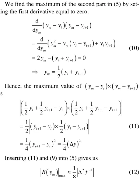
Hence, we need to know the maximal value of the re- mainder term nsider expressions (4) and (5). A
in (5). Co
ccording to expression (4) the remainder term is the difference between the linear interpolation zm and “true”
function value 1
m
f y . If we assume 1
f to be a smooth continuous function, the maximum error must occur where the f ’s curviness is m mum and this agrees with expression (5); the second derivative of
1
unction axi
f represents the curviness. Hence, we need to find the maximal value of
ymyi
ymyi1
in the segment of aximal curviness.First of all we ap derivative: m
proximate the second
2 1
2 1d f 1 2 2 d f (9)
We find the maximum of the second p ting the first derivative equal to zero:
f y
y y
art in (5) by set-
1
d
d m m i m i
y y y y
y
2 1 1 1 1 d d 2 0 1 2m m i i i i
m
m i i
m i i
y y y y y y
y
y y y
y y y
(10)
Hence, the maximum value of
ymyi
ymyi1
is
1 1 1 1 2 2 1 1 12 2 2 2
1 1
2 2
1 1
4 4
i i i i i i
i i i i
i i
y y y y y y
y y y y
y y y
(11)
Inserting (11) and (9) into (5) gives us
1 1 1
2 1max 8
m
R y 1 f (12)
Expression (12) should be calculated the function
in the segment of 1
f
d also lik
that has the greatest curviness.
[image:4.595.310.540.401.693.2]de
1.
(13)Hence, we can estimate the maximum of t
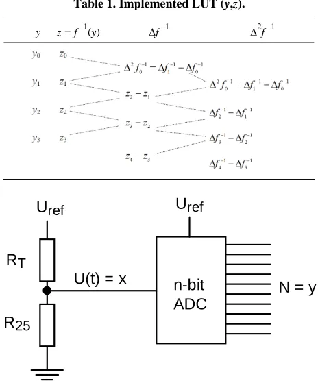
term from the LUT entries by the following expression: r term from data. Suppose we have implemented the LUT in Table
We can see that
1
1 11 2 1
i i i
i i i i
i i i
z z z z
z z z
2 1 1 1
f f f
he remainder
max 1 1 max1 2 8
m i i i
R y z z z (14)
4. Methods
We will illustrate the ideas suggested above with a case linearize a thermistor whose resistance temperature as follows [40]:
study. We will depends on the
25
1 1
exp
298
T
R R
T
where the temperature T is in Kelvin [K]. In a positive temperature coefficient and to
signal, we use the simple signal conditioning circuit in
(15)
[image:5.595.307.539.88.366.2]order to get get a voltage
Figure 6.
This will produce a voltage U(T) equal to
1U T
1 1
1 exp 298
ref
U T
(16)
and the ADC will produce an integer N according to
2
1
2
1 1
1 exp
298
n
ref
U
n
U T N
T f T
(17)
We get the inverse, linearizing function by solving for
T:
1
1
K
n
T f N
(18)
1 2 1
ln 1
298
N
In order to get some numbers to work with,
assign a typical value of 3000 K [40]. We will also assume that we use a 16-bit ADC. Hence, expression (18) is
we will
1
1
1 65536 1
T f N
(19)
ln 1
3000 N 298
Table 1. Implemented LUT (y,z).
y z = f –1(y) f –1 2f –1
R
TR
25U
refU
refU(t) = x
n-bit
ADC
N = y
Figure 6. Signal conditioning for non-linear thermistor. Ideally, we should store one LUT value for each value in the domain of N (0.65535), but we want to save me
- r
- m
te
ory space and decimate this table; we will estimate in mediate values by linear interpolation. According to (5), the interpolation error is proportional to the second derivative of expression (19). The second derivative cor- responds to the “curviness” of the function and since we are looking for the size of the maximum interpolation error, we will focus on the segments of 1
f that has the greatest curviness. Also, we can estimate the second de- rivative from data by using expression (13). In Figure 7
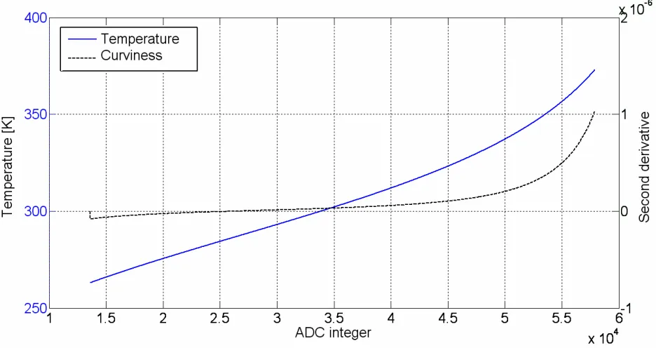
we have plotted both expression (19) and the second de- rivative from expression (13). As expected, the maximum of the second derivative occurs at the points of maximum curviness.
In Figure 7 we have only plotted the temperature for
N ranging from 13,602 to 57,889; this corresponds to an assumed temperature range of –10˚C to +100˚C.
5.
rviness, and hence the maximal interpolation errors, occurs at the
Empiri/Results
From Figure 7 we can see that the maximal cu
upper end of the f1 function. Hence, we only need to calculate expression (12) for the last N values in order to find the maximal interpolation error for any decimation factor.
[image:5.595.55.288.385.626.2]Figure 7. The function f–1 and its second derivative. Table 2. Maximal remainder term vs
r.
LUT decimation fac- to
Decimation factor Maximal remainder 1 1.2896 × 10⁻⁷
2 5.1553 × 10
4 2.0597 × 10⁻⁶ 8 8.2191 × 10⁻⁶
16 3.2720 × 10⁻⁵ 32 1.2965 × 10⁻⁴
64 5.0810 × 10⁻⁴ 128 2.0021 × 10⁻³
256 7.3008 × 10⁻³
–7
was calculat om expressions (12)
ble 2 should be compared to the byte ns in expressions (7) and (8).
ed fr and (13).
6. Discussion
The values in Ta
and word precisio
If we use the restraint that R y
m te , we can seefrom Table 2 and expression (7) that if we store LUT
en use a 16-bit
interpolation. If we store the LUT values as 16-bit words,
2 and expression (8) that a deci- mation factor of 8 will not affect the overall precision.
g an
rs in every digital system that rong or inaccurate LUT entries may nctions. As a matter of fact, it was a
linear inter- po
LUT size must be reduced to a minimum in order to we can see from Table
tries in 8-bit byte format and ADC, we can decimate the LUT by a factor of 64 without reducing the overall precision; the precision of the measurement esti- mate is still determined by the precision of the stored LUT entries, not by the errors introduced by the linear
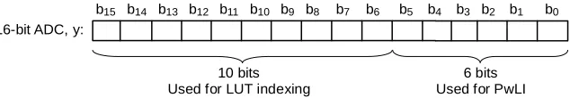
For the 8-bit case, we reduce the size of the LUT from 65 kbyte to only 1 kbyte which is a significant (and ab- solutely necessary) reduction of the LUT memory foot- print in a small embedded system. Of the 16-bit integer produced by the ADC, we use 10 bits for LUT indexin
d 6 bits for (piece-wise) linear interpolation. This is illustrated in Figure 8.
7. Conclusions
LUTs are used in a vast variety of applications [1-18] and the precision of LUT entries and the size of the LUT are crucial design facto
relies on LUTs. W cause serious malfu
LUT error that caused the infamous malfunction of In- tel’s Pentium processor in the mid 90’s [41].
This work has suggested a method for finding an op- timal LUT size when linearizing sensor outputs in small embedded systems. The idea is to use some of the (most significant) bits from the quantizer for LUT index ing and the rest of the (least significant) bits for
[image:6.595.56.289.391.563.2]10 bits Us
b15 b14 b13 b12 b11 b10 b8 b7 b6 b5 b4 b3 b2 b1 b0
ed for LUT indexing
6 bits Used for PwLI b9
[image:7.595.141.458.86.141.2]16-bit ADC, y:
Figure 8. LUT indexing and piece-wise linear interpolation. minimize the LUT memory footprint, which is absolutely
crucial in small embedded systems. This work has pre- sented a theory for finding th
emonstrated its use by a case study.
the original sam va
e optimal LUT size and d
The work is limited to the case were LUT entries are stored as integers since this is typically the case in small (8-bit) microcontrollers; the controller linearizes the sen- sor signal only, it does not estimate ple lue. We have argued that the interpolation error should be much less than the precision of the LUT entries. If the LUT entries are stored with m bits resolution we can es- timate their precision to be 2–m and if we use expressions (12) and (13) to estimate the interpolation error, we get the following general condition for determining the LUT size:
1 1 max
1
2 2
8
m
i i i
z z z (20)
REFERENCES
[1] W. Gawronski, F. Baher and E. Gama, “Track-Level- Compensation Look-Up Table Improves Antenna Poiting Precision,” 20
http://ipnpr.jpl rt/42-164/164E.pdf
eam Dumping System”, The 10th
In-Vol. 178, 2009, pp. 12-15. 06.
.nasa.gov/progress_repo
[2] R. A. Barlow, P. Bobbio, E. Carlier, G. Gräwer, N. Vou- mard and R. Gjelsvik, “The Beam Energy Tracking Sys- tem of the LHC B
ternational Conferences on Accelerators & Large Expe- riment Physics Control Systems,Geneva, 10-14 October, 2005, p. 02.056-4.
[3] P. Gaydecki, “New Real-Time Algorithms for Arbitrary, High Precision Function Generation with Applications to Acoustic Transducer Excitation,” Journal of Physics:
Conference Series,
doi:10.1088/1742-6596/178/1/012015
[4] P. Hung, H. Fahmy, O. Mencer and M. J. Flynn, “Fast Division with a Small Lookup Table,” 2002.
http://arith.stanford.edu/~hung/papers/asilomar.p
[5] M. D. Ercegovac, T. Lang, J.-M. Mu
df
ller and A.
Tisse-ultipliers,”
:10.1109/ARITH.1995.465382
rand, “Reciprocation, Square Root, Inverse Square Root and Some Elementary Functions Using Small M
IEEE Transactions on Computers, Vol. 49, No. 7, 2000, pp. 628-637.
[6] H. Hassler and N. Takagi, “Functions Evaluation by Ta- ble Look-up and Addition.” Proceedings of the 12th IEEE Symposium Computer Arithmetic, Bath, 19-21 July 1995, pp. 10-16. doi
mentary Functions in Single Precision,” IEEE Transac- tions on Computers, Vol. 44, No. 3, 1995, pp. 453-457.
[7] W. F. Wong and E. Goto, “Fast Evaluation of the Ele-
doi:10.1109/12.372037
[8] E. Balestrieri, P. Daponte and S. Rapuano, “A State of the Art on ADC Error Compensation Methods,” IEEE Trans- actions on Instrumentation and Measurement, Vol. 54, No. 4, 2005, pp. 1388-1394.
doi:10.1109/TIM.2005.851083
[9] A. C. Dent and C. F. N. Cowan, “Linearization of Ana- log-to-Digital Converters,” IEEE Transactions on Cir- cuits and Systems, Vol. 37, No. 6, 1990, pp. 729-737. doi:10.1109/31.55031
[10] M. Frey and H.-A. Loeliger, “On Flash A/D Converters with Low-Precision Comparators,” Proceedings ofIEEE International Symposium on Circuits and Systems, Greece, 21-24 May 2006, pp. 3926-3929.
/smash/get/diva2:19990/FULLTE
cGrath and R. D. Baer- [11] S. A. Jawed, “Analog-to-Digital Converter Design for
Non-Uniform Quantization,” Master Thesis, University of Linköping, Linköping, 2004.
http://liu.diva-portal.org XT01
[12] M. Pascale, “Microcontrollers CORDIC Methods”, 2004. http://www.drdobbs.com/184404244
[13] S. L. Gaverick, K. Fujino, D. T. M
tsch, “A Programmable Mixed-Signal ASIC for Power Metering,” IEEE Journal of Solid-State Circuits, Vol. 26, No. 12, 1991, pp. 2008-2016. doi:10.1109/4.104195
[14] E. Laulainen, L. Koskinen, M. Kosunen and K. Halonen, “Compass Tilt Compensation Algorithm Using CORDIC,”
tes/00687
ation on
er Characteristics to Measured Data,”
Proceedings of the 2008 IEEE International Symposium on Circuits and Systems, Vol. 1-10, 2008, pp 1188-1191. [15] M. Beckman and L. Chioye, “Precision Thermocouple
Measurement with the ADS1118,” Texas Instruments, 2011.
http://www.ti.com/lit/an/sbaa189/ sbaa189.pdf
[16] J. Julicher, “Simplified Thermocoupld Interfaces and PIC micro MCUs,” Microchip Technology, 2002.
[17] Mathworks, “Look-up Tables and Polynomials,” 2000. http://radio.feld.cvut.cz/matlab/toolbox/rtw/rtw_ug/opt_m od4.html
[18] B. C. Baker, “Precision Temperature-Sensing with RTD Circuits,” 2008.
http://ww1.microchip.com/downloads/en/appno c.pdf
[19] J. Day and S. Bible, “Piecewise Linear Interpol PIC12/14/16 Series Microcontrollers,” 2004.
http://ww1.microchip.com/downloads/en/AppNotes/0094 2A.pdf
IEEE Instrumentation & Measurement Magazine, Vol. 4, No. 4, 2001, pp. 26-39.
ntrollers,”
016/j.isatra.2010.04.004
[21] H. Erdem, “Implementation of Software-Based Sensor Li- nearization Algorithms on Low-Cost Microco
ISA Transactions, Vol. 49, No. 4, 2010, pp. 552-558. doi:10.1
94)00795-0
[22] P. Hille, R. Höhler and H. Strack, “A Linearisation and Compensation Method for Integrated Sensors,” Sensors and Actuators A, Vol. 44, No. 2, 1994, pp. 95-102. doi:10.1016/0924-4247(
11
i “New ADC with
t Humidity Sensor,” IEEE Transactions
1166.
asan, L. W. Adetunji, S. F. Abdulazeez, S. H. M. han, “On the Issue of
ure Sensor Design Guide”,
Micro-U zing Circuit,” Computers and Electronic
[23] “PIC32MX1XX/2XX Data Sheet,” Microchip Techno- logy Inc., 2011.
http://ww1.microchip.com/downloads/en/DeviceDoc/6 68D.pdf
[24] K. Post, “Interpolated Table Lookups Using SSE2 (1/2),” 2010.
http://rawstudio.org/blog/?p=457
[25] G. Bucci, M. Faccio and C. Land
Piecewise Linear Characteristic: Case Study—Implemen- tation of a Smar
on Instrumentation and Measurements, Vol. 49, No. 6, 2000, pp.
1154-[26] S. Khan, A. H. M. Z. Alam, S. M. Ahmmad, I. B. Tijani, M. A. H
Zaini, S. A. Othman and S. S. K
Linearizing a Sensor Characteristic over a Wider Re-sponse Range”, Proceedings of the International Confer- ence on Computer and Communication Engineering, Kuala Lumpur, 13-15 May 2008, pp. 72-76.
[27] Microchip, “Temperat chip Inc., 2009.
http://ww1.microchip.com/downloads/en/Device-Doc/21895d.pdf
[28] B. Trump, “Analog Linearization of Resistance Tempera- ture Detectors,” Analog Application Journal, Vol. 4Q, 2011, pp. 21-24.
[29] J. E. Brignell, “Software Techniques for Sensor Compensa- tion,” Sensors and Actuators A, Vol. 25, No. 1-3, 1991, pp. 29-35.
[30] B. Stringham, J. Leonard and S. Yakimchuk, “A sal Sensor Lineari
niver-
s in Agriculture, Vol. 4, No. 1, 1989, pp. 81-84.
doi:10.1016/0168-1699(89)90016-1
[31] D. K. Anvekar and B. S. Sonde, “Transducer Output Sig- nal Processing Using Dual and Triple Microprocessor Sys- tems,” IEEE Transactions on Instrumentation a
surement, Vol. 38, No. 3, 1989, pp. 8
nd Mea-
34-836. doi:10.1109/19.32204
[32] A. Flammini, D. Marioli and A. Taroni, “Transducer Output Signal Processing Using an Optimal Look-up Ta- ble in Microcontroller-Based Systems,” Electr
ters, Vol. 33, No. 14, 19
onics Let-
97, pp. 1197-1198. doi:10.1049/el:19970809
[33] A. Flammini, D. Marioli and A. Taroni, “Application of an Optimal Look-up Table to Sensor Data Processing,”
IEEE Transactions on Instrumentation and M
Vol. 48, No. 4, 1999, pp. 8
easurement, 13-816.
doi:10.1109/19.779179
[34] P. N. Mahana and F. N. Trofimenkoff, “Transducer Out- put Signal Processing Using an 8-Bit Microcontroller,”
IEEE Transactions on Instrumentatio
Vol. 35, No. 2, 1986, pp
n and Measurement, . 182-186.
eet,” Microchip Inc.,
orais, “Look-up Table and Breakpoints Determi- - putation,” IMTC 2003, Instrumen-
ahlquist,“Numeriska Me-
dition, McGraw-Hill, Singapore, 1990.
5. [35] “Sensors, Excitation and Linearization,” 2007.
http://media.wiley.com/product_data/excerpt/33/0780360 1/0780360133-2.pdf
[36] Microchip, “PIC18FXX8 Data Sh 2003.
http://www.micrchip.com/wwwproducts/Devices.aspx?d DocName=en010301
[37] S. Y. C. Catunda, O. R. Saavedra, J. V. FonsecaNeto and R. A. M
nation for Piecwise Linear Approximation Functions Us ing Evolutionary Com
tation and Measurement Technology Conference, Vail, 20-22 May 2003, pp. 435-440.
[38] L. Råde and B. Westergren, “Mathematics Handbook for Science and Engineering”, 3rd Edition, Studentlitteratur, Lund, 1995.
[39] P. Pohl, G. Eriksson and G. D
toder,” 5th Edition, ILiber Tryck, Stockholm, 1982.
[40] E. O. Doeblin, “Measurement Systems—Application and Design,” 4th E