The Effect of Financial Inclusion on Household Welfare in China

(1)

Munich Personal RePEc Archive

The Effect of Financial Inclusion on

Household Welfare in China

Mallick, Debdulal and Zhang, Quanda

Deakin University

August 2019

(2)

The Effect of Financial Inclusion on Household Welfare in China

Debdulal Mallick and

Quanda Zhang*

August 2019

Abstract:

Financial inclusion is one of the key factors contributing to household welfare. We explore this effect in China utilizing a unique household survey panel data. Financial inclusion is measured by owning a transaction account at formal financial institutions. We employ an innovative method of heteroscedasticity-based identification recently developed by Klein and Vella (2009a; 2010) to identify the causal effect of financial inclusion. We find that welfare effects of financial inclusion varied across urban and rural areas and income groups. Financial inclusion significantly increased overall consumption, but the impact was greater among urban than rural households. The effect was stronger in the case of food consumption. Financial inclusion also decreased consumption inequality but only among urban households. The uneven effect of financial inclusion across level of urbanization and commodity types have important policy implications for promoting financial inclusion not only in China but also in other developing countries.

Keywords: Financial inclusion; Consumption; Inequality; Welfare.

JEL Classification Codes: G21; I31; D14; D12.

(3)

1. Introduction

Financial inclusion is one of the most important factors contributing to the overall

economic development of a country. It creates opportunities for consumption smoothing,

especially for the poor, by acting as an insurance to build resilience against shocks. It also helps

get access to other basic needs such as education and health services, and is crucial for

investment opportunities for entrepreneurs (Bruhn and Love, 2009). The most significant

beneficiaries of financial inclusion are the marginalized and poor individuals, who lack this

opportunity at the first place (World Bank, 2019).

Notwithstanding its crucial role, financial inclusion has only recently gained attention

to the policymakers in both developing and developed countries.1_{Financial inclusion is}

sometimes confused with financial development and it is imperative to clarify the distinction

between the two concepts. Financial inclusion is characterized by households and businesses

using financial services. According to World Bank (2015), financial inclusion is defined as

“individuals and businesses have access to useful and affordable financial products and

services that meet their needs—transactions, payments, savings, credit and insurance—

delivered in a responsible and sustainable way.” Financial inclusion is measured at the micro

level by the access to financial instrument (such as transaction account) of an individual or a

household. Financial development, on the other hand, is a process of reducing the costs of

acquiring information, enforcing contracts and making transactions by establishing financial

institutions.2 Thus, the two concepts are quite distinct although there may be a high correlation

between them.

1

For example, in November 2015 the State Council of the Chinese government detailed the guiding principles

and goals in the Promoting Financial Inclusion Plan 2016-2020 to promote financial inclusion (The State Council

of P. R. China, 2015). In 2015, the United Kingdom established the Financial Inclusion Commission to promote

financial inclusion with two core objectives that include advocating financial inclusion as a public policy priority,

and working with policymakers and stakeholders to come up with deliverable policy proposals (The Financial

Inclusion Commission of the United Kingdom, 2015).

2

Financial development is usually measured by indicators such as the ratio of private credit, stock market

capitalization or M2 to GDP, and the number of ATMs or bank branches per capita. These aggregate indicators

are not informative about how individuals or households are able to take advantage of financial opportunities,

(4)

Research on the effect of financial inclusion on development outcomes at the individual

or household level is scant.3 Fitzpatrick (2015), using a household survey data for the

1995-2008 period for the UK, finds that owning a bank account improves access to credit (in terms

of credit card ownership) and increases consumption of household appliances. However,

Amendola, Boccia, Mele and Sensini (2016) failed to find any effect on the consumption of

non-durable goods. Zhang and Posso (2019) constructed an indicator of financial inclusion

using the information on transactions and payments, savings, credit and insurance, and find a

strong positive effect on household income in China.Dimova and Adebowale (2018), in the

context of Nigeria, find that financial inclusion, measured as owning a bank account, increases

per capita expenditure but also increases intra-household inequality. Adebowale and Lawson

(2018) find that financial inclusion reduces transient poverty in the same context as in Dimova

and Olabimtan (2018). DeLoach and Smith-Lin (2018), in the context of Indonesia, find that

financial inclusion measured in terms of access to savings and credit enables households to

borrow or liquidate assets in response to adult health shocks.4

In this paper, we investigate the effect of financial inclusion on different categories of

consumption and their inequality at the household level in China. To the best of our knowledge,

this is the first paper to investigate the impact of financial inclusion on these two important

welfare indicators at the household level. Given that consumption patterns vary across

households depending on, among others, their income level, investigation of different types of

consumption and also by income groups helps understand the beneficiaries of financial

inclusion. Understanding consumption inequality for different items is important because

inequality in consumption of necessary goods such as food are more worrying from welfare

perspectives than inequality in other types of consumption (Attanasio and Pistaferri, 2016). In

addition, investigation in the context of China is justified by its large share in the world

3_{Research has predominantly focused on the effect of financial development at the macroeconomic level. Some}

examples include, but not limited to, King and Levine (1993) on economic growth; Clarke et al. (2003) and Beck

et al. (2007) on income inequality; Burgess, Pande and Wong (2005) and Jalilian and Kirkpatrick (2005) on

poverty; Mallick (2014) on business-cycle volatility. Other notable works on this topic include, among others, Li

et al. (1998), Levine (2005), Beck and Demirgüç-Kunt (2008) and Jeanneney and Kpodar (2011). For a literature

review on the effect of financial development on inequality and poverty, see Zhuang et al. (2009).

4_{It is also important to appreciate that there is a large and vibrant literature on the effect of microfinance on many}

aspects of economic development ranging from poverty alleviation to women empowerment. However,

microfinance is a special type of financial inclusion targeted to a specific type of the population mainly by

(5)

population. Since the outline of the Promoting Financial Inclusion Plan 2016-2020 in

November 2015, various programs, such as establishing village banks and microcredit units,

have been implemented to promote financial inclusion throughout the country. By the end of

2017, five state-owned commercial banks, six joint-stock commercial banks, over 1600 rural

and county banks and 17 private banks in China had established financial inclusion division

(Li, Ye, Zeng and He, 2018). This signifies the importance of financial inclusion to the Chinese

government.

We analyze the China Household Finance Survey (CHFS) dataset for three waves—

2011, 2013 and 2015 (detailed discussion in Section 2) comprising a household level panel

dataset. The dataset contains detailed information on household financial products as well as

income, expenditures and a rich set of demographic characteristics. We focus on three broad

categories of consumption, namely, food, utilities and (non-food) necessities. To understand

the effect on overall consumption, we aggregate these three consumption categories. Financial

inclusion is measured by a binary variable indicating whether a household owns a transaction

account at any formal financial institution (that includes commercial bank, credit union and

postal bank, among others), which in our study context is mainly a bank. This measure is

consistent with the advocate and aim of the global financial inclusion movement. According to

the World Bank (2019), “being able to access a transaction account is a first step toward broader

financial inclusion” because a transaction account enables people to store money, and send and

receive payments. In other words, a transaction account serves as a gateway to other financial

services.5 For robustness check, we also augment the measure of financial inclusion by owning

a credit card.

Given the endogeneity of financial inclusion and that finding an external instrument is

a daunting challenge in our context, we employ an innovative identification method recently

developed by Klein and Vella (2009a; 2010) that does not rely on exclusion restriction but

exploits heteroscedasticity for identification (discussed in detail in Section 3.2). Our results

show that financial inclusion increases overall consumption by about 100%. The effect is

greater in urban (82%) than in rural areas (58%), and more pronounced among the lower

income households in urban areas. The effect is stronger in the case of food consumption. We

also find that financial inclusion decreases consumption inequality. The effect is limited only

5_{The Universal Financial Access 2020 Goal, initiated by The World Bank Group, envisions that by 2020, adults}

who currently are not part of the formal financial system, have access to a transaction account to store money,

(6)

in urban areas, especially the lower income households therein. There is no effect on

consumption inequality in rural areas. The uneven welfare improving effects of financial

inclusion across different level of urbanization and income groups have important policy

implications for promoting financial inclusion not only in China but also in developing

countries in general.

The rest of the paper proceeds as follows. Section 2 describes the data and reports some

key descriptive statistics. Empirical strategy including the identification method is explained

in Section 3. The results are presented in Section 4. Finally, Section 5 concludes and discusses

policy implications.

2. Data and Descriptive Statistics

Our analysis draws on the dataset from the China Household Finance Survey (CHFS).

The CHFS is a biennial longitudinal representative household survey developed by the Survey

and Research Center for China Household Finance at the South-Western University of Finance

and Economics (SWUFE). It employs a stratified three-stage Probability Proportion to Size

(PPS) random sample design. The first stage selected 80 counties out of the 2,585 primary

sampling units (including county level cities and districts) from all provinces and

municipalities in the mainland China except Hong Kong, Macau, Tibet, Xinjiang and Inner

Mongolia. The second stage selected four residential committees/villages from each of the 80

counties at the first stage. The third stage selected 20 to 50 households from each of the selected

residential committees/villages depending on the level of urbanization and economic

development. Every stage of sampling is carried with the PPS method and weighted by its

population size.6 The CHFS contains detailed information on household financial products,

income, expenditures and demographic characteristic of the households. In this study, we use

all available waves—2011, 2013 and 2015.7

We focus on three broad categories of consumption, namely, food, utilities and other

non-food necessities. Food refers to expenditures on all non-food items including dinning out. Utilities

refers to expenditures on water, electricity, fuel and property management fees.8 Necessities

6_{See Gan et al. (2014) for detailed description about this dataset.}

7_{We drop the top and bottom 5% of the observations based on total consumption because of non-reporting}

(missing values) and some households have unusually large ceremonial expenditure such as wedding.

8_{In some parts of China, especially in urban area, utilities bill can be paid through bank account. Electronic}

(7)

refers to non-food daily necessary items such as toiletries and detergent. The respondents were

asked to recall food and necessity expenditures for last 30 days from the day of the survey. We

include only these items to avoid any recall bias; expenditures on others items that are

purchased infrequently are harder to recall for the respondents, so there is a higher chance of

reporting bias. Note that utility bills are usually paid once a month and receipts are preserved

so that expenditures can easily be verified. All expenditures are annualized. For comparison

over time, each category of consumption is deflated by the respective CPI and separately for

rural and urban areas.9 We aggregate these three broad categories of (real) consumption to

construct the “total” consumption.

For each category of consumption (including the total), we construct inter-household

consumption inequality as:

2 ijt jt ijt jt C C CI C  −  = _ _   (1)

where C_ijt denotes consumption of household i of category j at time t, and C_jtis the median

consumption expenditure for each j. This measure of consumption inequality (CI) is similar to

the poverty measure in which a household’s consumption deviates from the poverty line

consumption. Poverty (headcount) index is calculated as the sum of the deviations across all

households; in our case, inequality at the household level is calculated as the deviation of an

individual household’s consumption from the median consumption. The deviation is squared

so that larger weight is assigned to the household whose consumption deviates more from the

median consumption.10 By construction, CI is symmetric around the median; two households,

one with consumption higher and another with consumption lower than the median

consumption by the same magnitude will have the same inequality score. Consumption

account minimizes transaction costs, such as costs of transportation and time to travel to the billing station, and is

also incentivized by utility providers and banks (or payment platforms) through discount on the amount to be paid

(Huang, 2019); this extra saving potentially allows people to spend more on utilities.

9_{Consumer Price Index are obtained from the National Bureau of Statistics of China}_{http://data.stats.gov.cn}

(accessed on 18 August 2019).

10

Note that without squaring, this CI index would simply be a transformation of Cijt, and would contain no

(8)

inequality decreases when consumption of a household moves closer to the median

consumption level.11

Our measure of financial inclusion is whether a household owns a transaction account at

any formal financial institution.12 We also augment this measure by including credit card

ownership—whether a household owns a transaction account or a credit card. We do not

consider credit card ownership separately as an alternative measure of financial inclusion as

only about 6% of the households in our data owned a credit card.

Insert Tables 1A and 1B

Table 1A provides some key descriptive statistics for all three surveys combined, and

Table 1B provides these by year. Sixty two percent of all sample households own a transaction

account.13_{The ownership is higher in urban than rural areas (70% vs. 47%) and remains almost}

the same between 2011 and 2013 and increases considerably in 2015 (from 57% in 2011 to

70% in 2015). Food consumption constitutes the major share in our measure of total

consumption as shown by the mean values of (logarithm) different categories of consumption

expenditures, which may be because of the items included in our study. All categories of

consumption increase over time, and are higher in urban than in rural areas. Consumption

inequality is greater in rural than urban areas, and more or less stable over time except for food

for which it is increasing.

3. Empirical Strategy

3.1. Empirical Specification

The empirical specification is given as:

ijt it r t ijt

Y = +

α β

FI +γ X′ _it + + +

λ τ ε

,

∀

j

(2)

11

This also holds when consumption of a household above the median decreases. However, we rule out this

possibility. We show that financial inclusion increases consumption of all types of households but benefits more

the households with lower level of consumption (see section 4.1 and Figures 1-4).

12

In many developing countries, transaction account is sometimes known as checking account or current account.

For example, in China, individuals can open a current account in a commercial bank, deposit and receive interests.

This account functions both as saving account and transaction account.

13_{In 2014, 62 percent of adults worldwide had an account at a bank or another type of financial institution or with}

(9)

where Y_ijt denotes the outcome (dependent) variables for household i of consumption category

j at time t—these are logarithm of consumption expenditure (C_ijt) and consumption inequality

defined in equation (1).

FI

_it refers to financial inclusion measuring access to financial

instruments in terms of owning a transaction account (for robustness check, we also include

credit card ownership). This is a binary variable equals 1 if a households owns a transaction

account and 0 otherwise.

λ

_r and

τ

_t are geographic region (such as province, rural-urban and

Hukou) and time fixed effects, respectively.14

Our key interest is β , the coefficient of

FI

_it. The extent to which a household is able

to consume and also achieve consumption smoothing depends on the tools at its disposal to

allocate resources over time. Transaction account is such a tool with which households are not

only able to absorb adverse shocks with their savings in it but also receive interpersonal and

government transfers. On the other hand, variation in the ownership of such tools may

potentially give rise to inequality in consumption. Looking at consumption inequality across

specific components of consumption is also interesting for a number of reasons. First, the

analysis of different type of commodities with different income elasticities can be useful to

understand the likely effects of the nature of shocks and about mechanisms for smoothing

consumption. Second, disparities in consumption of food and non-food necessary items may

be more concerning from a welfare point of view than disparities in the consumption of luxuries

(Attanasio and Pistaferri, 2016).

The vector

X

consists of demographic characteristics at the household level that

include age, gender and marital status of the household head, (average) education level of all

(adult) household members, family size, (log of) annual household disposal income and

14

Note that we do not include individual fixed effects in equation (2). In the data (also shown in Table 1.B), about

58% households have a bank account in all three periods (binary variable coded as 1), and about 30% households

did not have a bank account in any of the three periods (coded as 0). Therefore, for about 88% households,

financial inclusion (having a bank account or not) is a fixed effect (time invariant). The Fixed Effect (FE) (mean

differencing or LSDV) estimation will use information from only the remaining 12% households, for which

financial inclusion varies over time. The same applies to first-differencing estimation. We are indeed interested

in the coefficient of this (near) fixed effect, so controlling for individual fixed effect will discard most information

from the data. Our estimated coefficient is interpreted as the difference in the consumption between financially

included and excluded households (with and without owning a transaction account). On the other hand, the

coefficient estimated by FE regression would refer to the change in own consumption of a household after owning

(10)

political alignment (communist party membership). Income is considered to be the most

important factor determining household consumption. Although permanent income would be

more appropriate to determine current consumption (Friedman, 1957), such income measure is

unavailable, and we are unable to construct using our survey data. Therefore, we control current

income that includes salaries, revenues from family agricultural and/or business productions,

investment income, and transfer payments such as subsidies to maintain minimum living

standard for all household members. When consumption inequality is the dependent variable,

we also include a dummy variable indicating whether a household’s consumption is above or

below the median consumption.

Geographical factors (captured byλ_r ) are also important to determine household

consumption (and consumption inequality) and related to financial inclusion. These factors

include rural/urban, province and the Hukou. The Chinese economy is characterized by a

remarkable rural-urban division (Knight and Song, 1999). The rural areas lag far behind the

urban areas in terms of basic infrastructure such as roads, wastewater services, water supply

and sanitation. This uneven development in turn leads to uneven access to financial instruments

across rural and urban areas, and therefore, the effect of financial inclusion on outcome

variables might differ depending on the level of urbanization. The same argument applies to

provinces as well. Another reason for rural-urban division in China is the unique Hukou system

of household registration. Before the economic reform in 1978, the household register was used

mainly to control population mobility caused by food shortages. Households who could

produce their own food were classified as agricultural Hukou, and those who receive food from

the government were classified as non-agricultural Hukou. Traditionally, most agricultural

Hukou households live in rural areas and most non-agricultural Hukou households live in urban

areas. The strict restrictions on permanent migration from rural to urban Hukou and vice versa

is still in place in many parts of China. The Hukou system generates remarkable socioeconomic

gap between rural and urban residents because of government’s discriminatory policies.15

15_{The Hukou system has recently been reformed but the restrictions on permanent migration are still in place.}

Households registered in rural Hukou are allowed to move to urban Hukou (and indeed many households did) for

only temporary employment. It is also worth mentioning that rural-urban division and the Hukou division are not

(11)

3.2. Identification Strategy

The pooled panel OLS estimation of equation (2) will give biased and inconsistent

estimates of the β coefficient because of endogeneity of financial inclusion. Endogeneity may

arise from any or all of the following sources. There might be unobserved factors that

simultaneously influence a household’s access to finance and consumption expenditure.

Although we control for a rich set of variables including household income, these may not be

sufficient to account for all omitted variables. Higher demand for consumption may determine

someone’s decision to open a transaction account, thus leading to reverse causality. One might

argue that our proxy (owning a transaction account), although consistent with World Bank

(2015) definition of financial inclusion, may not fully capture the broader dimensions of

financial inclusion, and thus suffer from measurement error.16

To address the endogeneity, we need external instrument for financial inclusion but the

challenge is daunting to find a suitable instrument. We employ an innovative identification

strategy recently proposed by Klein and Vella (2009a; 2010; henceforth, K-V) that does not

rely on exclusion restrictions for identification but exploits heteroscedasticity to construct

instruments from the existing data.17 This method requires that the endogenous variable be

binary. It exploits non-spherical disturbances arising in the determination of the endogenous

variable. The main argument behind this identification is that, when there is substantial

heteroscedasticity in the equation relating the endogenous variable to the exogenous variables,

the changing variance in the residual acts as a “probabilistic shifter” of the endogenous variable.

Similar to the instrumental variables, this probabilistic shifter helps identify the causal

relationship between the dependent variable and the endogenous variable. Consider the

following equations (for consumption category j):

it it t it

Y

= +

α β

FI

+ Ζ +

δ

′

_i

ε

(3)

it it

FI

= + Ζ +

µ

γ

′

_it

u

, (4)

where

Y

_it is the consumption expenditure or inequality and

FI

_it is the financial inclusion.

Z

_i_t

includes the elements in vector

X

_i_tand the fixed factors in equation (2). Equations (3) and (4)

do not satisfy the exclusion restriction. However, Klein and Vella argue that β can be

16

We recognize that consumption can also be measured with errors. However, given that consumption is our

dependent variable, this measurement error does not affect the estimated coefficients.

17_{This method has also been employed by Berg, Emran and Shilpi (2013) and Millimet and Roy (2016), Bakshi,}

(12)

consistently estimated if the residuals

u

_it are heteroscedastic. Assume that residuals are

heteroscedastic in the following way:

( )

it u t it

u =S Z_i u , (5a)

( )

it Sε t it

ε

= Zi

ε

(5b)

where

u

_itand

ε

_itare zero mean homoscedastic residuals, Z_i_t is a subset of (or equal to)

Z

_i_t,

and Su(Zit) is a non-constant positive function. The requirement for identification is that some

residuals are heteroskedastic in that Su(Zit) /Sε(Zit) varies across observations and the

conditional correlation between the underlying homoscedastic portion of the residuals is

fixed.18

We can write equation (4), where the probability of the financial inclusion (binary

endogenous indicator) is given by

Pr( 1) ( ) p t it u t FI P S   = =     i i Z Z 

 , (6)

where P(.) is the distribution function for

u

_it. With homoscedastic errors, S_u(Z_i_t) is a constant,

and identification depends on possible non-linearity of the P(.) function, such as normal

distribution. However, this identification relies on a small fraction of the data because it is

based on the non-linearity in the tails of the distribution, and hence, in general, not considered

as credible. In contrast, when there is heteroscedasticity, the function S_u(Z_i_t) is not a constant,

and identification exploits data from the region where P(.) is linear. The variables

( ) t u t S i i Z Z  

determine financial inclusion of a household but do not affect the mean impact of financial

inclusion on household consumption (or consumption inequality) specified in equation (3).

Therefore, conditional on heteroscedasticity in the residuals, the predicted probability of

equation (6) works as a valid instrument of the binary endogenous variable (Klein and Vella,

2009a; 2010).

18

Note that both S_u(Z_i_t)and S_ε(Z_i_t)are written as a function of Z_i_t, but there is no restrictions on which

(13)

In our estimation, we assume (following Millimet and Roy, 2016, and Farré et al., 2013)

that the heteroskedastic functions follows Su(Zit)=exp(−Z′ittiθ). We implement the K-V

estimator as follows. First, we estimate equation (4) by heteroskedastic probit regression to

generate the predicted probability of financial inclusion (variables generating

heteroscedasticity discussed in next section).19 This predicted probability is then employed as

an instrument for the binary financial inclusion. Therefore, our endogeneity correction follows

three stages in which the background (or zero) stage involves generating the instrument, and

then estimating the standard 2SLS method employing the instrument constructed in the

background stage.

4. Results and Discussions

4.1 Pooled OLS Estimation: The Effect on Consumption

The results are presented in Table 2 for the full sample and also disaggregated by the

rural and urban samples. In all cases and for all categories of consumption, the coefficient of

financial inclusion is positive and significant at any conventional level. For example, in the full

sample financially included households (that is owning a transaction account) has about 14%

higher consumption than financially excluded households. Among different categories, the

highest effect of financial inclusion is found on food consumption in all samples. However,

these results are biased and inconsistent because of endogeneity of financial inclusion

discussed in Section 3.2.

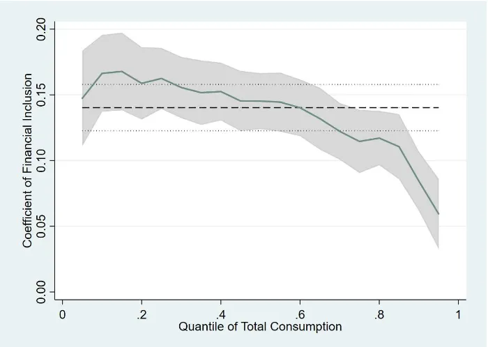
Insert Table 2 and Figures 1-4 here

Before presenting endogeneity-corrected results, we estimate the effect for different

quantiles, which will be crucial to explain our results for the consumption inequality. The

quantile regression results are displayed in Figures 1-4. As shown in Figure 1, the effect of

financial inclusion, although positive and significant for quantiles, secularly diminishes with

higher level of consumption. The same is true for food and utility consumption (Figures 2 and

19_{Similar steps have also been followed by Berg, Emran and Shilpi (2015) and}Bakshi, Mallick and Ulubaşoğlu

(14)

3 respectively). In the case of (non-food) necessity consumption, the effect varies across

consumption quantiles but the pattern still weakly holds. Although these results clearly indicate

that financial inclusion decreases consumption inequality, endogeneity correction is required

for a proper assessment that we conduct in Section 4.2.2.

4.2 Heteroscedasticity-based IV estimation

Before presenting the results, it is imperative to discuss the construction of the

instrument at the background stage. Ideally, variables that are considered to generate

heteroscedasticity are included in Z , but identifying these variables is not always an easy task.

Therefore, several studies, including Klein and Vella (2009b), include all variables in the Z

vector in the background stage (Z=Z ) that we also follow in our baseline estimation.

Nonetheless, we need to understand mechanisms through which (some of) these variables in Z

contribute to heteroscedasticity.

Households differ in their access to financial services depending on the overall

economic and financial development of where they reside. Given the level of development in

a particular location/region, households also differ in their access to financial services

depending on their economic and demographic characteristics.

In any country, level of economic development is usually not uniform across regions.

In the case of China, this is more pertinent as, even with increasing contribution of the private

sector, development process is still heavily regulated and planned by the government. For

example, regions especially in the coastal areas are more industrialized than the rest of the

country (a notable example is creation of the export processing zones); access to banking and

other financial institutions is also greater in these regions. Another source of regional disparity

is the Hukou (discussed in the previous section), which is a unique household registration

system in China that restricts migration within the country. The rural Hukous are very much

underdeveloped compared to their urban counterparts, and households registered in one type

of Hukou are not generally allowed to permanently migrate to another type, thus permanently

dividing households in their financial inclusion. Therefore, the geographic variations are

potentially important factors contributing to heteroscedasticity.

At the household level, income is one of the most important factors that generates

heteroscedasticity; higher income households need better access to financial institutions to

(15)

transactions, thus education is another factor that potentially generate heteroscedasticity across

households in their access to financial institutions.20

Insert Table 3 here

To verify the above arguments in the data, we first estimate equation (4) by the

heteroscedasticity probit regression by including all of the explanatory variables, that is, Z=Z.

We find that income, education, and geographic variation (province and Hukou) are among the

factors contributing to residual variance (Column 2 in Table 3). The results are in line with our

arguments above. Additionally, we find that family size and marital status also contribute to

heteroscedasticity. In our robustness exercise, we include only these significant variables as

the sources of heteroscedasticity at the background stage (i.e., Z_i_t) to construct instrument. To

reconfirm their role in contributing to heteroscedasticity, we re-estimate the heteroscedasticity

probit model including only these variables and find that their contributions remain robust in

this alternative specification (Column 3 in Table 3).21 The null hypotheses of homoscedasticity

of the residuals are rejected at any conventional level in both cases.

4.2.1 IV Estimation: The Effect on Consumption

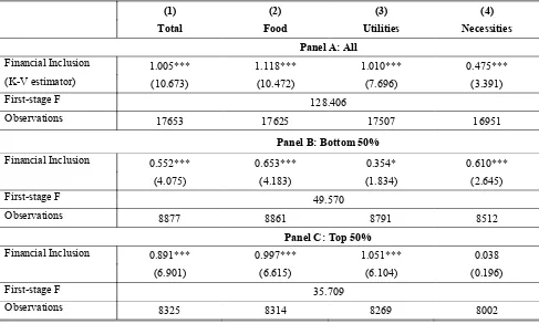
The results for the full sample are presented in Table 4.1, Panel A. The coefficient of

financial inclusion is positive, large in magnitude and statistically significant at any

conventional level. In the case of total consumption, the coefficient is 1.01 implying that

financially included households have about 100% higher consumption than financially

excluded households. The effect varies across different consumption categories ranging from

the highest 112% for food to the lowest 48% for (non-food) necessities. To understand if the

20

Sen and De (2018) argue that in India the poor are constrained to access banking because of their financial

illiteracy and adverse geographical location. Therefore, even though they get government social welfare benefits

through their bank accounts, they spend less on children education compared to the households receiving cash

transfers.

21

When the heteroscedasticity probit model is estimated separately for rural and urban, and by income groups,

the variables generating heteroscedasticity are not uniform across specifications. The variables that generate

heteroscedasticity in each case are mentioned in the notes for Tables B1.1 to B2.3 in Online Appendix B. We do

not report the heteroscedasticity probit regression for these cases, but it must be mentioned that in all cases the

(16)

effects vary across income groups, we estimate the results separately for households in the

bottom and top 50 income percentiles. Panels B and C report the results for these two income

groups, respectively. The coefficients of FI are larger for the top 50 income percentile

compared to bottom 50 income percentile for all categories of consumption except necessities

although for both groups the magnitudes are smaller compared to those in the full sample. It is

worth mentioning that the background stage regressions to construct the instrument are

estimated separately for each income percentile. The 2SLS estimations give different LATE

(local average treatment effect) estimates for the two groups and therefore they are not strictly

comparable.22

Insert Tables 4.1-4.3 here

Given that rural and urban households differ greatly in terms of their financial inclusion

(discussed in Section 2, also Table 1), and also that rural-urban disparity in economic

development is enormous in China (discussed in Section 3), we now estimate the results for

the rural and urban samples separately.23 The results for the rural sample are presented in Table

4.2. Financial inclusion increases total, food and necessary consumption by 58%, 80% and

56%, respectively, but there is no effect on utilities (Panel A). In the urban sample, financial

inclusion increases all categories of consumption, and magnitude of the coefficients are larger

than those obtained in the rural sample (Table 4.3). These magnitudes are comparable with

those in Fitzpatrick (2015) who found that financial inclusion increases consumption of

household appliances by 62%, and Dimova and Adebowale (2018) who found that financial

inclusion increases per capita expenditure by 62%-67%.

There is also economic inequality (and consequently variation in financial inclusion)

within both rural and urban areas and it is more severe in urban areas (Gustafsson, Shi and

Sicular, 2008). When the rural sample is disaggregated by bottom and top 50 income

percentiles, we do not find any effect in either income percentiles (Table 4.2, Panels B and C).

In contrast, the effect in the urban sample is significant only in bottom 50% income percentile

(Table 4.3, Panels B and C).

22

The magnitudes of the LATE estimates are also not comparable with the OLS estimates in Table 2, which are

much smaller. Fitzpatrick (2015) also reported big differences in these two sets of estimates.

23

We divide our sample into rural and urban following the classification from the National Bureau of Statistics

(17)

In general (Table 4.1-4.3), the effect of financial inclusion on consumption is greater

on food than other two categories. The effect is greater in urban than rural areas and more

pronounced among the lower income households in urban areas.

The instruments constructed in the background stage are relevant in all cases. This is

evaluated by the values of the F-statistics in the first-stage regressions that regress the

endogenous variable (financial inclusion) on the instrument (and the set of controls) that these

are well above 10 in all cases (Stock, Wright and Yogo, 2002).

4.2.2 IV Estimation: The Effect on Consumption Inequality

We construct the consumption inequality for each category j separately for full, rural,

urban and different income groups. It is worth reiterating that CI in equation (1) is symmetric

around the median, and consumption inequality decreases when consumption of a household

moves closer to the median consumption level (see footnote 11). However, in Section 4.1 (and

Figures 1-4), we have shown that the effect of financial inclusion is larger for households with

lower level of consumption and secularly decreases with consumption. Therefore, a negative

coefficient on FI in the regression of consumption inequality would imply that financial

inclusion benefits more (less) the households below (above) the median consumption level.

Insert Tables 5.1-5.3 here

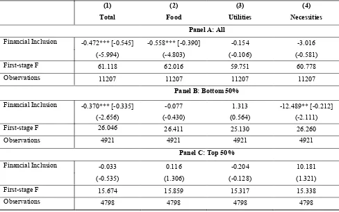
The results for the full sample are presented in Tables 5.1 (Panel A). The coefficients

of financial inclusion are negative and statistically significant suggesting that financial

inclusion benefits more to the households below than above the median consumption level.

Although the estimated coefficients differ by large magnitudes (ranging from -0.34 to -9.3)

across different consumption categories, their standardized coefficients (reported in brackets)

differ by smaller magnitudes. One standard deviation increase in access to financial instrument

decreases consumption inequality by about 0.15 percentage points in the case of food and

necessities, respectively, and 0.26 percentage points for utilities. This inequality-reducing

effect is more pronounced among the top 50 income percentile; for them inequality decreases

for food and utilities, while for the bottom 50 income percentile inequality decreases for

necessities (Panels B and C).

However, financial inclusion has no effect on consumption inequality in the rural

(18)

and when further disaggregated by income percentiles, it decreases for utilities in the case of

bottom 50 income percentile (Table 5.3, Panels B and C).

In all cases, the F-statistic from the first-stage regressions are well above 10

suggesting the relevance of the instrument.

4.2.3 Robustness Checks

We check the robustness of the benchmark results discussed in Sections 4.2.2 and 4.2.3

in a variety of ways. Our first two robustness checks retain the same measure of financial

inclusion. The first exercise involves including the squared value of original instrument as an

additional instrument (see, Millimet and Roy (2016) for a similar exercise). These results are

presented in Online Appendix A. For the second robustness exercise, we construct instrument

by including only those variables in the background stage regression that are found to generate

heteroscedasticity (see Section 4.2). The results are presented in Online Appendix B. Finally,

we augment the measure of financial inclusion as owning a transaction account or a credit card.

It is important to note that in almost all cases households owning a credit card also own a

transaction account. For example, 62% of the sample households own a bank account, while

63% own either a bank account or credit card. There is no considerable difference between

urban and rural areas in terms of the two measures of financial inclusion (70% vs. 72% in urban;

47% vs. 48% in rural). The results are presented in Online Appendix C. In all cases, the results

are strongly robust to the benchmark results both in terms of the magnitudes of the coefficients

of financial inclusion and their significance level.

4.2.4 Overtime Changes in Consumption Inequality

The previous results document that financial inclusion decreases consumption

inequality. The effect is pronounced in the case of food consumption. From welfare perspective

it is also important to understand whether consumption inequality changes over time. Our panel

data allows us to address this issue by separately analyzing the three waves of survey—2011,

2013 and 2015.

Insert Table 6 here

The results are summarized in Table 6. We estimate only for the full sample to exploit

a large sample size, and report only the standardized coefficients. The effect on total

(19)

inclusion decreased consumption inequality by 0.73 percentage points in 2011, while the same

change in financial inclusion decreased consumption inequality by 0.35 and 0.37 percentage

points in 2013 and 2015, respectively. More importantly, the effect on food consumption

inequality ceases to exist in subsequent periods. These results suggest that the diminishing

effects over time of financial inclusion. This may be due to smaller scope for further reducing

consumption inequality once it is already low, a concept similar to diminishing marginal

returns. For other two consumption categories, there is no clear pattern.

5. Concluding Remarks

The impact of financial inclusion on household welfare is a very relevant but an

unexplored area of research. This paper investigates this important question in the context of

China. It uses a unique dataset that contains three waves of household survey and corrects the

endogeneity of financial inclusion employing an innovative method developed by Klein and

Vella that does not rely on exclusion restrictions but exploits heteroscedasticity to estimate the

causal effect.

The results indicate that financial inclusion almost doubles household consumption.

This effect is greater in developed urban than underdeveloped rural areas. In general, the effect

is stronger for food consumption. Financial inclusion decreases inequality in overall and food

consumption, but this effect is concentrated mainly to the urban households. These findings

are very important from welfare perspectives signifying the crucial role played by financial

inclusion since inequality in food consumption is more concerning than inequality in

consumption in durable or luxury goods. Although, we did not investigate the consumption of

durable and luxury goods, it would be an interesting extension for further research.

Regional or geographic (including rural vs. urban) variation in the impact on

consumption and its inequality is a direct consequence of uneven development. In this regard,

the role of the government is to ensure the universal opportunity for financial inclusion for all

citizens. A prominent example is The Prime Minister’s Jan Dhan Yojana (PMJDY), a scheme

launched in 2014 by the Indian government, to ensure, among others, universal access to

banking facilities with at least one basic bank account for every household, financial literacy

and access to credit, insurance and pension facility (PMJDY, 2019). The impact of such

universal financial inclusion initiative on household welfare, especially on inequality, would

(20)

References

Adebowale, Olabimtan, and David Lawson (2018). 2018. “How Does Access to Formal

Finance Affect Household Welfare Dynamics? Micro Evidence from Nigeria.” GDI Working

Papers 2018-024. The Global Development Institute: Manchester, UK.

Amendola, Alessandra, Marinella Boccia, Gianluca Mele, and Luca Sensini (2016), “Financial

Access and Household Welfare.” The World Bank Policy Research Working Papers 7533. The

World Bank: Washington DC.

Attanasio, Orazio P., and Luigi Pistaferri. 2016. “Consumption Inequality.” Journal of

Economic Perspectives 30(2):3–28.

Berg, Claudia, M. Shahe Emran, and Forhad Shilpi. 2013. “Microfinance and Moneylenders:

Long-run Effects of MFIs on Informal Credit Market in Bangladesh.” The World Bank Policy

Research Working Papers 6619.The World Bank: Washington DC.

Bruhn, Miriam, and Inessa Love. 2009. “The Economic Impact of Banking the Unbanked:

Evidence from Mexico.” The World Bank Policy Research Working Paper 4981. The World

Bank: Washington DC.

Bakshi, Rejaul K., Debdulal Mallick, and Mehmet A. Ulubaşoğlu. 2019. “Social Capital as a

Coping Mechanism for Seasonal Deprivation: The Case of the Monga in Bangladesh.”

Empirical Economics 57(1): 239-262.

Beck, Thorsten, Asli Demirgüç-Kunt, and Ross Levine. 2007. “Finance, Inequality and the

Poor.” Journal of Economic Growth 12(1): 27-49.

Beck, Thorsten, and Asli Demirgüç-Kunt. 2008. “Access to Finance: An Unfinished Agenda.”

The World Bank Economic Review 22(3): 383-396.

Burgess, Robin, Rohini Pande, and Grace Wong. 2005. “Banking for the Poor: Evidence from

(21)

Clarke, George, Lixin Colin Xu, and Heng-fu Zou. 2003. “Finance and Income Inequality: Test

of Alternative Theories.” The World Bank Policy Research Working Paper 2984. The World

Bank: Washington DC.

DeLoach, Stephen B., and Marquessa Smith-Lin. 2018. “The Role of Savings and Credit in

Coping with Idiosyncratic Household Shocks.” Journal of Development Studies 54(9):

1513-1533.

Demirguc-Kunt, Asli, Leora Klapper, Dorothe Singer, and Peter Van Oudheusden. 2015. “The

Global Findex Database 2014: Measuring Financial Inclusion around the World.” The World

Bank Policy Research Working Papers 7255. The World Bank: Washington DC.

Dimova, Ralitza, and Olabimtan Adebowale. 2018. “Does Access to Formal Finance Matter

for Welfare and Inequality? Micro Level Evidence from Nigeria.” Journal of Development

Studies 54(9): 1534-1550.

Farré, Lídia, Roger Klein, and Francis Vella. 2013. “A Parametric Control Function Approach

to Estimating the Returns to Schooling in the Absence of Exclusion Restrictions: An

Application to the NLSY.” Empirical Economics 44(1): 111-133.

Fitzpatrick, Katie. 2015. “The Effect of Bank Account Ownership on Credit and Consumption:

Evidence from the UK.” Southern Economic Journal 82(1): 55-80.

Friedman, Milton. 1957. A Theory of the Consumption Function. Princeton, NJ: Princeton

University Press.

Gan, Li, Zhichao Yin, Nan Jia, Shu Xu, Shuang Ma, and Lu Zheng. 2014. Data You Need to

Know about China. Heidelberg, Germany: Springer.

Gustafsson, B.A., Li Shi, and Terry Sicular. 2008. Inequality and Public Policy in China.

Oxford, UK: Oxford University Press.

(22)

http://epaper.voc.com.cn/sxdsb/html/2019-04/29/content_1386046.htm?div=-1 [accessed on

August 5 2019]

Jalilian, Hossein, and Colin Kirkpatrick. 2005. “Does Financial Development Contribute to

Poverty Reduction?” Journal of Development Studies 41(4): 636-656.

Jeanneney, Sylviane G., and Kangni Kpodar. 2011. “Financial Development and Poverty

Reduction: Can There be a Benefit without a Cost?" Journal of Development Studies 47(1):

143-163.

Klein, Roger, and Francis Vella. 2009a. “A Semiparametric Model for Binary Response and

Continuous Outcomes under Index Heteroscedasticity.” Journal of Applied Econometrics

24(5): 735-762.

Klein, Roger and Francis Vella. 2009b. “Estimating the Returns to Endogenous Schooling

Decisions via Conditional Second Moments” Journal of Human Resources, 44(4), pp.

1047-1065

Klein, Roger, and Francis Vella. 2010. “Estimating a Class of Triangular Simultaneous

Equations Models without Exclusion Restrictions.” Journal of Econometrics 154(2): 154-164.

King, Robert G., and Ross Levine. 1993. “Finance and Growth: Schumpeter Might be Right.”

The Quarterly Journal of Economics 108(3): 717-737.

Knight, John, and Lina Song. 1999. The Rural-Urban Divide: Economic Disparities and

Interactions in China. Oxford, UK: Oxford University Press.

Levine, Ross. 2005. “Finance and Growth: Theory and Evidence.” in: Philippe Aghion &

Steven Durlauf (ed.), Handbook of Economic Growth, edition 1, volume 1, chapter 12, pages

865-934 Elsevier.

Li, Hongyi, Lyn Squire, and Heng-fu Zou. 1998. “Explaining International and Intertemporal

(23)

Li, Yang, Zhenzhen Ye, Gang Zeng, and Xia He, ed. 2018. China Financial Inclusion

Innovation Report (2018). Beijing, China: Social Sciences Academic Press.

Mallick, Debdulal. 2014. “Financial Development, Shocks, and Growth Volatility.”

Macroeconomic Dynamics 18(3): 651-688.

Millimet, Daniel L., and Jayjit Roy. 2016. “Empirical Tests of the Pollution Haven Hypothesis

when Environmental Regulation is Endogenous.” Journal of Applied Econometrics 31(4):

652-677.

PMJDY. 2019. “About: Pradhan Mantri Jan-Dhan Yojana.” Government of India.

https://www.pmjdy.gov.in/about. [accessed on August 5 2019]

Sen, Gitanjali, and Sankar De. 2018. “How Much Does Having a Bank Account Help the

Poor?.” Journal of Development Studies 54(9): 1551-1571.

Stock, James H., Jonathan H. Wright, and Motohiro Yogo. 2002. “A Survey of Weak

Instruments and Weak Identification in Generalized Method of Moments.” Journal of Business

and Economic Statistics 20 (4): 518–29.

The State Council. 2015. Promoting Financial Inclusion Plan 2016-2020. Beijing, China: The

State Council of the People’s Republic of China.

The Financial Inclusion Commission. 2015. Financial Inclusion: Improving the Financial

health of the Nation. London, UK: The Financial Inclusion Commission.

World Bank. 2015. Global Financial Development Report 2015/2016: Long-term Finance.

Washington DC: The World Bank.

World Bank. 2019. “Financial Inclusion”. Washington D.C., The World Bank.

http://www.worldbank.org/en/topic/financialinclusion/overview. [accessed on August 5 2019]

(24)

Zhuang, Juzhong, Herath Gunatilake, Yoko Niimi, Muhammad Ehsan Khan, Yi Jiang, Rana

Hasan, Niny Khor, Anneli S. Lagman-Martin, Pamela Bracey, and Biao Huang. 2009.

“Financial Sector Development, Economic Growth, and Poverty Reduction: A Literature

Review.” Asian Development Bank Economics Working Papers 173. Asian Development

(25)

[image:25.595.76.527.136.581.2]

Tables and Figures

Table 1A: Descriptive statistics

Variable Full sample Urban Rural T-test

Mean SD Mean SD Mean SD p value

Annual expenditures on food (log) _9.223 _0.766 _9.454 _0.648 _8.822 _0.788 0.000

Annual expenditures on utilities

(log) 7.352 0.909 7.622 0.779 6.883 0.929 0.000

Annual expenditures on non-food

daily necessities (log) 6.661 1.014 6.827 0.989 6.379 0.993 0.000

Annual total expenditures (log) _9.500 _0.692 _9.722 _0.585 _9.115 _0.694 0.000

Consumption inequality of food _0.428 _0.587 _0.404 _0.661 _1.753 _4.044 0.000

Consumption inequality of utilities _1.110 _6.557 _1.343 _8.167 _4.011 _27.062 0.000

Consumption inequality of

necessities 1.664 12.518 4.466 32.592 4.881 31.666 0.000

Consumption inequality of total _0.370 _0.477 _0.301 _0.398 _1.072 _2.395 0.000

Annual household disposable

income (log) 10.362 1.222 10.596 1.158 9.957 1.224 0.000

Owning a transaction account

(1=yes; 0=no) 0.616 0.486 0.699 0.459 0.471 0.499 0.000

Average education level 3.448 1.381 3.886 1.417 2.688 0.905 0.000

Household size 3.626 1.602 3.331 1.411 4.137 1.777 0.000

Gender of hh head 0.785 0.411 0.735 0.441 0.873 0.333 0.000

Marital status of the hh head

(1=married; 0=otherwise) 0.905 0.293 0.896 0.305 0.920 0.271 0.000

Rural Hukou (1=yes; 0=no) 0.559 0.497 0.339 0.473 0.940 0.237 0.000

Communist party membership

(1=yes; 0=no) 0.209 0.406 0.265 0.441 0.111 0.314 0.000

Data sources: CHFS 2011, 2013, 2015 and authors’ calculation. Λ: Inequality calculated using Equation (1) in the

(26)

[image:26.595.74.562.353.601.2]

Table 1B: Summary statistics of some key variables by year

Variable 2011 2013 2015

Mean SD Mean SD Mean SD

Transaction Account _0.577 _0.494 _0.592 _0.491 _0.698 _0.459

Food exp (log) _9.125 _0.763 _9.289 _0.744 _9.283 _0.780

Utilities exp (log) _7.192 _0.935 _7.408 _0.899 _7.510 _0.848

Necessity exp (log) _6.323 _0.936 _6.808 _0.997 _6.936 _1.009

Total exp (log) _9.367 _0.698 _9.572 _0.670 _9.601 _0.679

CIfood _0.521 _0.826 _0.714 _1.123 _0.889 _1.424

CIutilities _2.020 _10.481 _2.267 _12.699 _2.815 _18.509

CInecessities _4.092 _34.700 _2.495 _16.408 _3.853 _25.489

CItotal _0.514 _0.792 _0.517 _0.766 _0.487 _0.686

Income _10.138 _1.195 _10.471 _1.218 _10.548 _1.215

Table 2: The impact of financial inclusion on consumption (pooled OLS)

(1) (2) (3) (4)

Total Food Utilities Necessities

Panel A: Full Sample

Financial Inclusion _0.140*** _0.153*** _0.096*** _0.129***

(15.117) (14.299) (7.245) (8.350)

Observations ₁₇₆₅₃ ₁₇₆₂₅ ₁₇₅₀₇ ₁₆₉₅₁

Panel B: Rural Sample

(9.222) (8.710) (3.746) (5.900)

Observations ₆₄₄₆ ₆₄₃₆ ₆₃₈₄ ₆₂₅₉

Panel C: Urban Sample

(11.220) (10.508) (6.099) (5.827)

Observations ₁₁₂₀₇ ₁₁₁₈₉ ₁₁₁₂₃ ₁₀₆₉₂

(27)

[image:27.595.61.536.90.459.2]

Table 3: Background stage regression: Identifying variables generating heteroscedasticity

*, **, *** represent significance level at 1, 5, 10 percent level, respectively. Robust t-statistics reported in parentheses.

Variable Level Residual Squared Residual Squared

(1) (2) (3)

Income _0.139*** _-0.069*** _-0.070***

(4.071) (-4.117) (-4.210)

Education _0.147*** _0.112*** _0.106***

(3.872) (5.535) (5.648)

Size _-0.035*** _0.041*** _0.042***

(-3.447) (2.736) (2.838)

Male _0.058** _-0.026

(2.347) (-0.537)

Marry _0.002 _-0.142** _-0.153**

(0.062) (-2.021) (-2.225)

Hukou _-0.074*** _0.008

(-2.659) (0.122)

Communist Party _0.049* _-0.058

(1.803) (-1.100)

Year Fixed Effects Yes Yes Yes

Rural-Urban Fixed Effects Yes Yes Yes

Province Fixed Effects Yes Yes Yes

Background Stage: Heteroskedastic Probit

LR test of homoscedasticity χ2_{and p-value}

122.052

0.000

120.48

(28)

[image:28.595.73.560.101.394.2]

Table 4.1: The impact of financial inclusion on consumption (full sample)

(1) (2) (3) (4)

Panel A: All

(K-V estimator) _(10.673) _(10.472) _(7.696) _(3.391)

First-stage F _128.406

Observations ₁₇₆₅₃ ₁₇₆₂₅ ₁₇₅₀₇ ₁₆₉₅₁

Panel B: Bottom 50%

Financial Inclusion _0.552*** _0.653*** _0.354* _0.610***

(4.075) (4.183) (1.834) (2.645)

Observations ₈₈₇₇ ₈₈₆₁ ₈₇₉₁ ₈₅₁₂

Panel C: Top 50%

Financial Inclusion _0.891*** _0.997*** _1.051*** _0.038

(6.901) (6.615) (6.104) (0.196)

Observations ₈₃₂₅ ₈₃₁₄ ₈₂₆₉ ₈₀₀₂

(29)

[image:29.595.75.569.100.431.2]

Table 4.2: The impact of financial inclusion on consumption (rural sample)

(1) (2) (3) (4)

Panel A: All

Financial Inclusion _0.576*** _0.797*** _0.403 _0.554*

(2.692) (3.138) (1.313) (1.677)

First-stage F 36.310

Observations ₆₄₄₆ ₆₄₃₆ ₆₃₈₄ ₆₂₅₉

Financial Inclusion _0.253 _0.371 _-0.124 _-0.201

(1.145) (1.488) (-0.402) (-0.633)

Observations ₂₉₀₂ ₂₈₉₆ ₂₈₆₉ ₂₇₉₀

Financial Inclusion _0.219 _0.309 _0.364 _0.307

(1.164) (1.415) (1.489) (1.107)

Observations ₂₈₈₅ ₂₈₈₂ ₂₈₆₅ ₂₈₂₃

(30)

[image:30.595.73.560.100.403.2]

Table 4.3: The impact of financial inclusion on consumption (urban sample)

(1) (2) (3) (4)

Panel A: All

Financial Inclusion _0.822*** _0.914*** _0.628*** _0.362**

(7.805) (7.723) (4.162) (2.111)

Observations ₁₁₂₀₇ ₁₁₁₈₉ ₁₁₁₂₃ ₁₀₆₉₂

Financial Inclusion _0.702*** _0.628*** _0.940*** _0.665**

(4.536) (3.769) (4.168) (2.529)

Observations ₄₉₂₁ ₄₉₁₃ ₄₈₇₅ ₄₆₈₃

Financial Inclusion _0.164 _0.138 _-0.032 _0.234

(1.318) (0.930) (-0.186) (0.941)

Observations ₄₇₉₈ ₄₇₉₂ ₄₇₆₈ ₄₅₅₂

(31)

[image:31.595.74.560.100.402.2]

Table 5.1: The impact of financial inclusion on consumption inequality (full sample)

(1) (2) (3) (4)

Panel A: All

Financial Inclusion _{-0.885*** [-0.571]} _{-0.344* [-0.149]} _{-7.448*** [-0.261]} _{-9.332** [-0.166]}

(-6.882) (-1.881) (-2.905) (-2.368)

First-stage F _129.817 _129.512 _125.621 _127.403

Observations ₁₇₆₅₃ ₁₇₆₅₃ ₁₇₆₅₃ ₁₇₆₅₃

Financial Inclusion _{-0.967*** [-0.364]} _-0.458 _-0.491 _{-24.780*** [-0.286]}

(-2.810) (-1.055) (-0.077) (-3.218)

First-stage F _51.798 _50.944 _48.666 _49.864

Observations ₈₈₇₇ ₈₈₇₇ ₈₈₇₇ ₈₈₇₇

Financial Inclusion _{-0.310*** [-0.407]} _{-0.166* [-0.159]} _{-4.110*** [-0.234]} _-7.152

(-4.485) (-1.875) (-3.220) (-1.453)

First-stage F _35.713 _36.227 _34.818 _35.353

Observations ₈₃₂₅ ₈₃₂₅ ₈₃₂₅ ₈₃₂₅

Robust t-statistics in parentheses: *, **, *** represent significance level at 1, 5, 10 percent level, respectively. Standardized coefficients in brackets—reported only for statistically significant coefficients.

(32)

[image:32.595.72.560.101.402.2]

Table 5.2: The impact of financial inclusion on consumption inequality (rural sample)

(1) (2) (3) (4)

Panel A: All

Financial Inclusion _-0.980 _-0.324 _10.041 _-9.988

(-1.063) (-0.216) (0.570) (-1.441)

First-stage F _37.727 _38.001 _36.124 _36.217

Observations ₆₄₄₆ ₆₄₄₆ ₆₄₄₆ ₆₄₄₆

Financial Inclusion _-0.387 _-0.505 _20.369 _-4.271

(-0.324) (-0.256) (0.632) (-0.919)

First-stage F _14.857 _14.884 _14.441 _14.683