A multilevel latent Markov model for the evaluation of nursing homes' performance

Munich Personal RePEc Archive

A multilevel latent Markov model for the

evaluation of nursing homes’ performance

Montanari, Giorgio E. and Doretti, Marco and Bartolucci,

Francesco

Department of Political Science, University of Perugia, Department

of Political Science, University of Perugia, Department of

Economics, University of Perugia

8 August 2017

A multilevel latent Markov model for the

evaluation of nursing homes’ performance

Giorgio E. Montanari

, Marco Doretti

, and Francesco Bartolucci

1

_{Department of Political Science, University of Perugia}

_{Department of Economics, University of Perugia}

August 8, 2017

Abstract

The periodic evaluation of health care services is a primary concern for many in-stitutions. In this work, we focus on nursing home services with the aim to produce a ranking of a set of nursing homes based on their capability to improve - or at least to keep unchanged - the health status of the patients they host. As the overall health status is not directly observable, latent variable models represent a suitable approach. Moreover, given the longitudinal and multilevel structure of the available data, we rely on a multilevel latent Markov model where patients and nursing homes are the first and the second level units, respectively. The model includes individual covariates to account for the patient case-mix and the impact of nursing home membership is modeled through a pair of correlated random effects affecting the initial distribution and the transition probabilities between different levels of health status. Through the prediction of these random effects we obtain a ranking of the nursing homes. Fur-thermore, the proposed model is designed to address non-ignorable dropout, which typically occurs in these contexts because some elderly patients die before completing the survey. We apply our model to the Long Term Care Facilities dataset, a longi-tudinal dataset gathered from Regione Umbria (Italy). Our results are robust to the sensitivity parameter involved (the number of latent states) and show that differences in nursing homes’ performances are statistically significant.

Keywords: clustered data, health status evaluation, non-ingorable dropout, random effects

1

Introduction

Due to population aging, the demand of health care services from elderly people is

con-stantly increasing in many occidental countries (White, 2007; Gray, 2009). As a

conse-quence, the proper evaluation of the offered services has become a key matter of

govern-ments, at national and regional level. Among these services, nursing home care is one of

the most relevant (Makai et al., 2014).

In this work, we develop a statistical model to compare the performance of different

nursing homes operating in the same context. As an illustration we apply such a model to

the health care system of Umbria, a region of central Italy, where a specific public protocol

namedLong Term Care Facilities (LTCF) has been implemented for many years. As part of

the LTCF program, a questionnaire is periodically administered to elderly patients hosted

in regional nursing homes (NHs) in order to monitor their overall health status. Thus, a

longitudinal dataset is available for many purposes. Specifically, our aim is to use such a

database for developing methods of evaluation of the ability of a nursing home to preserve

its patients in good health conditions.

For longitudinal multivariate data, latent Markov (LM) models represent an interesting

approach when the response variables are categorical and are assumed to measure some

underlying characteristic (Bartolucci et al., 2013). This class of models was first introduced

by Wiggins (1973) and has become quite popular for this kind of data. In its classical

formulation, an LM model assumes that the response variables (typically resulting from

the administration of a questionnaire) are affected by an unobserved process evolving over

time according to a first-order discrete-time Markov chain with a finite number of states.

This unobserved process represents the latent trait of interest, which in our application

viewed as the counterpart of the latent class model (Goodman, 1974) for longitudinal data

in which each latent class (or latent state) corresponds to a different level of the health

status. Many extensions of the basic LM model have been proposed in the literature to

account for additional information, represented by individual covariates, or specific data

structures; see for example Vermunt et al. (1999). In this paper, we develop a multilevel

latent Markov (MLM) model with covariates to deal with the hierarchical structure of the

LTCF data (i.e., patients hosted in different nursing homes). The nursing home effect on

the health status of their patients is represented by a pair of random effects assumed to

affect the distribution of the initial latent state and the transition probabilities between

latent states across time. As a matter of fact, our final goal is to rank the nursing homes

based on their performance in improving or maintaining their patients’ conditions as good

as possible.

Though the multilevel extension of the latent class model has been widely discussed

and applied in the literature; see, among the others, Vermunt (2003), Henry and Muth´en

(2010), Montanari et al. (2010), and Gnaldi et al. (2016), its longitudinal counterpart,

namely the MLM model, is not as much widespread. To the best of our knowledge, just

a few authors have adopted it as a modeling strategy in their applications. For instance,

Bartolucci et al. (2011) focus on educational data, while Koukounari et al. (2013) consider

the MLM model for the analysis of longitudinal datasets in the medical context. In these

papers, the multilevel structure is accounted for by means of cluster-specific time-fixed

random effects. Bartolucci and Lupparelli (2016) extend this approach using cluster random

effects with a time-varying structure, specifically, a Markov chain. In any case, a discrete

distribution over a finite number of support points is specified for the random effects.

On the contrary, in this work we adopt a continuous distribution. This strategy permits

(i.e., nursing homes) in a more explicit way with respect to models that, being based on

discrete random effects, provide a clustering of such units. There are also advantages in

terms of stability of the parameter estimates, being the proposed model more parsimonious

than the counterpart based on discrete random effects. Continuous random effects have

been already introduced in this field within the so-called class of mixed hidden Markov

models (Altman, 2007; Maruotti, 2011; Maruotti and Rocci, 2012). However, often these

random effects are intended as means to capture unobserved heterogeneity between units

rather than accounting for multilevel data structures.

Bartolucci et al. (2009) propose a similar framework with the aim of evaluating nursing

home performances. They also use an LM model with covariates to assess the effect of

nursing homes on the probability of transition between latent states through fixed effects

introduced by a suitable set of dummy explanatory variables. However, the estimation

of these NH effects is rather unreliable - when not unfeasible - if as in our case some

NHs contain just a few units. Furthermore, the model proposed here also accounts for

dropout due to the death of patients, which is a common problems arising in this type of

applications. Ignoring the missing data mechanism may lead to biased estimates. Overall,

up to our knowledge, the application of an MLM model to the present context (multivariate

longitudinal data with missing values) is innovative.

The outline of the paper is as follows. In Section 2 we present in detail the LTCF data

considered in our analysis. The proposed MLM model is illustrated in Section 3, while

model results are reported in Section 4. Main conclusions are given in Section 5 together

2

The LTCF dataset

The data motivating the proposed approach come from the Suite interRAI questionnaire,

an internationally validated and widely adopted tool (Hirdes et al., 2008; Kim et al., 2015).

Our sample refers to the years 2012 and 2013 and contains 1,292 individuals grouped in

47 different NHs. The questionnaire is planned to be administered approximately every

six months so that, ideally, four measurement occasions - one for each semester of the two

years - should be present for each patient. However, only 3,924 instead of 5,168 (4×1,292) observations are available. This is due to either intermittent missingness, when a patient

does not respond at a given measurement occasion but responds at a following occasion,

or dropout, due to patients leaving the study before scheduled because of death or other

causes. Intermittent missingness involves a modest, though not negligible, proportion of

observations (204, approximately 5%). Dropout has a more severe impact as it concerns

439 individuals (34% of the sample). About the reasons for dropout, death occurs in 377

cases (86%); other reasons are discharge or transfer to other structures such as hospitals.

A description of how such missingness mechanisms are taken into account is provided in

Section 3.2.

We have to note that, although observations of each patient are expected to be collected

every six months, the time intervals between observations show a variability related to the

evolution of patients’ health conditions. Observations are sometimes anticipated in the

presence of some change in these conditions, or delayed in the opposite case.

The entire Suite interRAI questionnaire is divided in several sections referring to

dif-ferent spheres of the health status, which in general is a multidimensional phenomenon.

However, in this paper we focus on a single section of the questionnaire. This section is an

the difficulty patients experience in taking common actions. Specifically, the ADL section

includes ten items, which are described in Table 1. Focussing only on the ADL implies

that the latent trait we consider represents just patients’ physical condition in a strict

sense. This approach might be perceived as limiting, because other important aspects of

the health status (cognitive conditions, humoral status, etc.) are not included in the

anal-ysis. However, it permits to represent the latent trait as a unidimensional variable having

a meaningful interpretation.

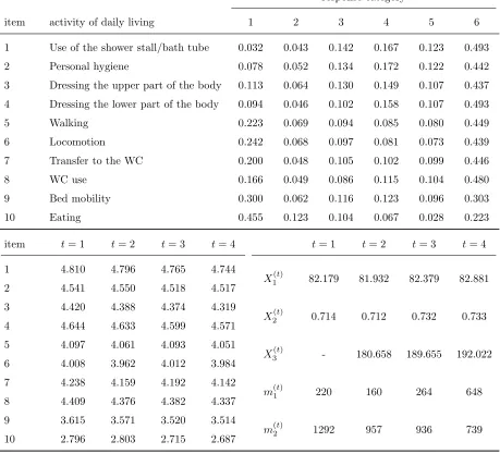
The response variables are measured on an ordinal scale with 6 categories (1-6), from no

difficulty at all to complete dependence on other people. In the upper part of Table 1, for

each ADL item we report the frequency distribution of the response categories referred to

all the 3,924 observations. In the bottom-left-hand side we report the item average response

(i.e., the mean of the category labels weighted with their frequencies) for each time occasion

t = 1, . . . ,4. Note that, although one expects an increase in the ADL difficulties over time, this is not the case because of dropout. In the bottom-right-hand side of Table 1, we also

report for each time the average patients’ age (X₁(t)), the proportion of females (X₂(t)), the average time interval in days between the current and the previous observation (X₃(t)), the number of patients with t observations (m(₁t)), and the number of patients surveyed at the

t-th occasion (m(₂t)).

3

The multilevel latent Markov model

In this section, we present the MLM model. Here, we introduce the main notation, while the

model specification, including how the missing data mechanism is formulated, is illustrated

in Sections 3.1 and 3.2. Finally, Section 3.3 describes the maximum likelihood estimation

response category

item activity of daily living 1 2 3 4 5 6

1 Use of the shower stall/bath tube 0.032 0.043 0.142 0.167 0.123 0.493 2 Personal hygiene 0.078 0.052 0.134 0.172 0.122 0.442 3 Dressing the upper part of the body 0.113 0.064 0.130 0.149 0.107 0.437 4 Dressing the lower part of the body 0.094 0.046 0.102 0.158 0.107 0.493 5 Walking 0.223 0.069 0.094 0.085 0.080 0.449 6 Locomotion 0.242 0.068 0.097 0.081 0.073 0.439 7 Transfer to the WC 0.200 0.048 0.105 0.102 0.099 0.446

8 WC use 0.166 0.049 0.086 0.115 0.104 0.480

9 Bed mobility 0.300 0.062 0.116 0.123 0.096 0.303 10 Eating 0.455 0.123 0.104 0.067 0.028 0.223 item t= 1 t= 2 t= 3 t= 4 t= 1 t= 2 t= 3 t= 4 1 4.810 4.796 4.765 4.744

X₁(t) 82.179 81.932 82.379 82.881 2 4.541 4.550 4.518 4.517

3 4.420 4.388 4.374 4.319

X₂(t) 0.714 0.712 0.732 0.733 4 4.644 4.633 4.599 4.571

5 4.097 4.061 4.093 4.051

X₃(t) - 180.658 189.655 192.022 6 4.008 3.962 4.012 3.984

7 4.238 4.159 4.192 4.142

m(t)₁ 220 160 264 648 8 4.409 4.376 4.382 4.337

9 3.615 3.571 3.520 3.514

m(t)₂ 1292 957 936 739 10 2.796 2.803 2.715 2.687

As typical in a multilevel analysis, we have n sample units divided into H different clusters. Therefore, every unit is characterized by a double index hi, with h = 1, . . . , H

and i = 1, . . . , nh, where nh is the dimension of the h-th cluster so that n = PH_h=1nh.

Furthermore, we denote by Y_hi(t) the response vector of unit i in cluster h at occasion t. This vector consists of J univariate categorical responses, that is Y_hi(t) = (Y_hi(t₁), . . . , Y_hiJ(t)). Each univariate response Y_hij(t) might have a generic number of categories cj, j = 1, . . . , J.

Moreover, every unit hi can have a specific number of measurement occasions Thi ≤ T,

where T denotes the maximum number of occasions observed in the sample for a unit. The vectorsY_hi(t) can be collected across time in the vector Yhi= (Y

(1)

hi , . . . ,Y

(Thi)

hi ). In

turn, we let Yh = (Yh1, . . . ,Yhnh) be the vector of all observations of cluster h. Individual

covariates are denoted by X_hi(t), and similarly to the response variables we set Xhi =

(X_hi(1), . . . ,X(Thi)

hi ) and Xh = (Xh1, . . . ,Xhnh). Every individual-specific Markovian latent

process is denoted by Vhi = (V

(1)

hi , . . . , V

(Thi)

hi ), where, at each time occasion t, V

(t)

hi is

a categorical variable with k levels. Again, individual latent processes within the same cluster can be collected in the vector Vh = (Vh1, . . . ,Vhnh). Finally, we denote the vector

of cluster-specific random effects, which are time invariant, with Uh = (Wh, Zh).

3.1

Model formulation

In the MLM model, the latent processes of two different clusters - say Vh and Vh′ - are

considered independent. As a consequence, the vectors Y₁, . . . ,YH collecting the responses

at cluster level are marginally independent. However, for units in the same cluster h, the independence is conditional on the cluster random effect Uh. Moreover, the Markovian

structure governing the latent individual processes Vhi is assumed to hold conditionally

on the cluster random effect Uh and on individual covariates Xhi. This means that the

process. Specifically, we define the conditional initial probabilities as

π_hi(1)(v) = P(V_hi(1) =v|X_hi(1) =x(1)_hi, Wh =wh), v = 1, . . . , k,

and the conditional transition probabilities as

π_hi(t)(v|v¯) = P(V_hi(t) =v|V(t−1)

hi = ¯v,X

(t)

hi =x

(t)

hi, Zh =zh), v,v¯= 1, . . . , k, t = 2, . . . , Thi,

where Wh and Zh are the two components of Uh already defined above. Notice that we

are implicitly assuming that Zh is independent of V_hi(1) given (X_hi(1), Wh) and that Wh is

independent of V_hi(t) given (V(t−1)

hi ,X

(t)

hi, Zh) for t = 2, . . . , Thi. Also, Uh is assumed to be

marginally independent of Xh. Such conditional initial and transition probabilities are

collected into individual-specific vectors

π_hi(1) =π_hi(1)(1), . . . , π(1)_hi(k)

and matrices

Π(_hit) = 

   

π(_hit)(1|1) . . . π_hi(t)(k|1) ... . .. ...

π_hi(t)(1|k) . . . π(_hit)(k|k) 

   

, t= 2, . . . , Thi.

Their dependence on cluster membership and individual covariates is modeled by the

re-gression equations

logπ

(1)

hi (v+ 1) +· · ·+π

(1)

hi (k)

π_hi(1)(1) +· · ·+π_hi(1)(v) =ξv +x

(1)

hiβ+whσw, v = 1, . . . , k−1 (1)

and

log π

(t)

hi(v + 1|v¯) +· · ·+π

(t)

hi(k|v¯)

π_hi(t)(1|¯v) +· · ·+π_hi(t)(v|¯v) =ψv¯+ωv+x

(t)

hiγ+zhσz, v = 1, . . . , k−1, ¯v = 1, . . . , k,

for t= 2, . . . , Thi.

In Equations (1) and (2), a global logit parametrization is assumed; see Bartolucci et al.

(2009) for more details about this parametrization applied in a similar context. Under this

parametrization, the covariate effects, represented by the column vectors β and γ, are

constant across the logit equations, while the sequences of thresholds ξ1 ≥ · · · ≥ξk−1 and ω1 ≥ · · · ≥ωk−1 must be non-increasing to ensure that the cumulative sums of probabilities

along the ordered categories of the latent variables are non-decreasing. On the contrary,

no order restrictions are posed on the sequence ψ1, . . . , ψk. However, ψ1 = 0 is set for

identification purposes.

A standard bivariate normal distribution with correlation coefficient ρ is assumed for the cluster effect random vector Uh. The overall variability of the clustering process is

governed by the parameters σw and σz in (1) and (2). These parameters are obviously

constrained to be non-negative in the estimation phase (see Section 3.3). The higher (and

the more statistically significant) their deviations from zero, the higher the relevance of

clustering in the data (and therefore the necessity to account for it).

Individual covariates and cluster effects are assumed not to enter in the measurement

model, that is, in the model for the outcomes given the latent process. In the present

context, this assumption allows to interpret the latent statesv = 1, . . . , k as different levels of seriousness of patients’ conditions. As a matter of fact, each outcome Y_hij(t) is assumed to be independent of any other variable in the model conditionally on V_hi(t). Under this setting, the relevant parameters are the conditional response probabilities

φjyjv =P(Y

(t)

hij =yj|V

(t)

hi =v),

with j = 1, . . . , J, yj = 1, . . . , cj, and v = 1, . . . , k. Notice that these probabilities are not

the conditional response probabilities can be stored in the matrix

Φj =



   

φj11 . . . φjcj1

... ... ...

φj1k . . . φjcjk



   

, j = 1, . . . , J.

However, the number of unconstrained conditional response probabilities is rather high

even in relatively small settings.

In order to make the model more parsimonious, several different parametrizations can

be imposed. Also in this case, we adopt a global logit parametrization of type

log φj,m+1,v+· · ·+φjcjv

φj1v +· · ·+φjmv

=τjm+δv, (3)

for j = 1, . . . , J, m = 1, . . . , cj −1, and v = 1, . . . , k. As in (1) and (2), in Equation (3)

the sequences of thresholds τj1 ≥ · · · ≥ τj,cj−1 must be non-increasing for j = 1, . . . , J.

Moreover, δ1 is set to 0 to ensure model identifiability and δ1 ≤ · · · ≤ δk is imposed

in order to obtain a positive association between the responses and the latent variable.

In this way, we can tackle the label switching problem, that is typical of discrete latent

variable models (see, e.g., Stephens, 2000). Notice that this parametrization provides a

clear interpretation of the latent states and is appropriate as the latent variables V_hi(t) have an ordinal nature.

3.2

Missing data modelling

As already shown in Section 2, in the LTCF dataset we consider there is a relatively large

proportion of missing data. Therefore, a careful evaluation of the missingness mechanism

is needed. On one hand, intermittent missingness and dropout due to reasons other than

the other hand, dropout due to death is very often associated to a worsening in patients’

health conditions. Therefore, the former can be treated as ignorable (Little and Rubin,

2002), while the latter clearly cannot, and an explicit model needs to be set for it.

Dropout due to death is modeled by expanding the available set of observations.

Specif-ically, for each response j, we add an extra response category cj + 1 in a way such that

data trajectories for patients dead after thet-th occasion (t < T) are completed by setting

Y_hij(u) =cj + 1 for u=t+ 1, . . . , T. A similar approach was undertaken also by Montanari

and Pandolfi (2016). In our application, the total number of observations raises from 3,924

to 4,746 after this expansion. We also define an extra latent state k+ 1 corresponding to death, which may be seen as an extreme health condition. Some of the extra probabilities

generated by this adjustment are suitably constrained. Specifically, we have:

• π_hi(1)(k+ 1) = 0 for all h and i: no one can be in the extra death state at the first occasion;

• π_hi(t)(v|k+ 1) = 0 andπ_hi(t)(k+ 1|k+ 1) = 1 for allhand i, andt= 2, . . . , T: no one can revert to other latent states after being in the extra death state (also called absorbing

state);

• φj,cj+1,v = 0, v = 1, . . . , J, and φj,cj+1,k+1 = 1 for all j: only the extra response

category can be observed if one is in the extra latent state.

Thus, initial probability vectors and transition matrices take the form

π(1)_hi =π_hi(1)(1), . . . , π(1)_hi(k),0

, Π(_hit)=        

π_hi(t)(1|1) . . . π_hi(t)(k|1) π_hi(t)(k+ 1|1) ... . .. ... ...

π(_hit)(1|k) . . . π_hi(t)(k|k) π_hi(t)(k+ 1|k)

0 0 0 1

while each conditional response matrix becomes

Φj =

       

φj11 . . . φjcj1 0

... ... ... 0

φj1k . . . φjcjk 0

0 0 0 1

        .

Clearly, π_hi(t)(k+ 1|1), . . . , π(_hit)(k+ 1|k) are the only unconstrained additional probabilities our dropout correction entails to estimate. These are the probabilities of transition to the

death state, given the patient is in a generic latent statev at the previous occasion, forv = 1, . . . , k. According to the adopted parametrization, this corresponds to the estimation of the single additional thresholdωk, withωk ≤ωk−1: the probabilities which are constrained

to zero or one are obtained by introducing new thresholds taking values equal to −∞

or +∞, respectively. Finally, the model extension we propose to deal with missing data involves only one free parameters to estimate: the additional threshold ωk.

3.3

Maximum likelihood estimation

Denoting by p1 =|β| and p2 =|γ| the number of individual covariates affecting the initial

and transition probabilities, the total number of free model parameters is

p= 4k+p1+p2+

J

X

j=1

(cj −1).

Specifically, we have:

• k−1 +p1 parameters for the initial probabilities;

• PJ

j=1(cj −1) +k−1 parameters for the conditional response probabilities;

• 3 parameters for the cluster random effect.

Putting all these parameters in a single vector θ, the model log-likelihood is expressed by

ℓ(θ) =

H

X

h=1

logP(Yh =yh|Xh =xh). (4)

Computing the above log-likelihood obviously requires the computation of the

cluster-specific probabilities P(Yh =yh|Xh =xh). The model assumptions imply that

P(Yh =yh|Xh =xh) =

Z

R2

"_nh Y

i=1

P(Yhi =yhi|Xhi =xhi,Uh =uh)

#

φ(uh;0,Σ)duh, (5)

where φ(uh;0,Σ) denotes the density function at uh of a bivariate normal distribution

with null mean and variance-covariance matrix

Σ=   1 ρ ρ 1  ,

with ρ being the correlation between the two componentsWh and Zh ofUh. For every hi,

P(Yhi=yhi|Xhi=xhi,Uh =uh) may be computed by the Baum-Welch forward recursion (Baum et al., 1970; Welch, 2003). To compute the integral in (5), we rely on a bivariate

quadrature approximation (Press et al., 1989) based on the following steps. First, by a

Gauss-Hermite method we define Q quadrature points ν∗

q and the corresponding weights

λ∗

q (q = 1, . . . , Q) for the standard bivariate normal distribution (with ρ = 0). Then, to

account for the correlation ρ we let

νq=Lνq∗, λq =λ∗q, q = 1, . . . , Q,

where Lis the Choleski decomposition of Σ. Finally, we use the approximation

P(Yh =yh|Xh =xh)≈ Q X q=1 "_n h Y i=1

P(Yhi=yhi|Xhi=xhi,Uh =νq)

#

In our application, we consider 11 quadrature points for each dimension, so that a grid of

Q = 112 _{= 121 points is obtained overall. This approximation is reasonable and higher}

values would result in prohibitive computational times.

Parameter estimates ˆθ are obtained from direct maximization of the log-likelihood. For

this aim we rely on a BFGS algorithm (Fletcher, 1987), which is available in the statistical

software R. In order to run this algorithm, the approximate log-likelihood gradient must

be calculated; see Supplementary material Section 1 for details on how to compute this

gradient. The BFGS algorithm also returns the Hessian matrix containing the numerical

second derivatives ofℓ(θ) at the maximum likelihood estimate ˆθ. Therefore, the estimated variance-covariance matrix is readily available to compute standard errors for the parameter

estimates.

In the end it is worth clarifying some aspects about the implementation of the maximum

likelihood estimation. First of all, the whole maximization algorithm is run using suitable

transformations of the random effect parameters σw, σz, and ρ. Specifically, logarithmic

transformations for σw and σz are introduced to ensure these parameters are positive (see

Section 3.1). Moreover, a Fisher transformation F(ρ) = 1/2 log[(1 +ρ)/(1−ρ)] is used for

ρ so that its final estimate is ensured to lie between -1 and 1 (Fisher, 1915). The variance-covariance matrix of these parameters on the original scale, namely prior to transformations,

can be easily approximated by using the Delta method (Oehlert, 1992). Moreover, as any

iterative algorithm, the BFGS needs to start from an initial guess for the parameter vector

θ. In this regard we recall that for complex latent variable models, as that object of the

present paper, multimodality of the likelihood function may arise and this leads to a lack

of uniqueness of the maximum likelihood solution. A typical solution consists in trying

different initializations for the estimation algorithm. In our application, we mainly follow

LM model with cluster-level fixed effects (Bartolucci et al., 2009), which is performed by an

Expectation Maximization algorithm (Dempster et al., 1977), and lettingσw =σz = 1 and

ρ= 0 as starting values. In fact, given the complexity of the model, trying many different starting values may be prohibitive in terms of computing time for large values of k. In any case, we tried different starting values which were randomly generated and we found

that the initial solution based on the preliminary fitting of the fixed-effects LM model is

typically better than other solutions.

4

Results

In this section, we summarize the results from the fitting of the MLM model on the LTCF

data. We recall that in this dataset n = 1,292 patients are divided in H = 47 NHs. Moreover, there are J = 10 categorical outcomes with the same number of categories, that is, cj = c = 6 for j = 1, . . . , J. Finally, because of intermittent missing data and

dropout we have a varying number of measurement occasions Thi≤T = 4 for each patient.

Age, age squared, gender, and time interval between occasions are considered as individual

covariates (see Section 2). Clearly, the last covariate covariate is included only in the model

for transition probabilities (see Equation (2)) and not in the model for initial probabilities.

In this way we account for the variability of the time length between consecutive time

occasions for the same individual. Typically, one is interested in six-month ahead transition

probabilities, as six months is the interval between measurements originally designed in the

LTCF study, though deviations from this target are observed.

In the reminder of this section, we first provide an outline of the procedure we adopted

for model selection (Section 4.1). Then, results for the selected models are reported

4.1

Model selection

As typical in the latent variable framework, model selection is essentially concerned with

the choice of the number of latent statesk. This decision requires a preliminary exploration of a range of different values of k. In this application, we fit models with k from 2 to 7. We avoid higher values ofk as it is known that models with many latent states often result in some of the generated subgroups having a reduced dimension and collecting sample

units with a behavior very far different from the majority of the sample. Typically, these

spurious subgroups do not represent real segments of the population under investigation,

and their existence is due to overfitting only. Moreover, fork > 7 the threshold constraints of Section 3.1 are unlikely to be met without additional model structure.

One way to account for model complexity is to rely on classical information criteria

based on the log-likelihood penalization. Specifically, here for every model we compute the

Bayesian Information Criterion (BIC, Schwarz, 1978), defined as

BIC =−2ℓ( ˆθ) +plogn,

where n is the number of sample units and p is the overall number of free parameters. In principle, models with a lowerBIC should be preferred. However, this index is often prone to favor models with too many latent states; see Bacci et al. (2014) for a detailed comparison

of different selection criteria in a similar context. Therefore, it is a good practice to also

consider alternative criteria. For instance, one could assess how sharp the posterior (i.e.,

given the data) classification of units into the latent states is. Formally, letting

˜

v_hi(t) = max

v=1,...,kP(V

(t)

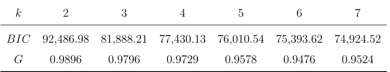
k 2 3 4 5 6 7

BIC 92,486.98 81,888.21 77,430.13 76,010.54 75,393.62 74,924.52

G 0.9896 0.9796 0.9729 0.9578 0.9476 0.9524

Table 2: Values of BIC and G for models with k∈2, . . . ,7

for the MLM a measure of the sharpness of a k-state model’s classification is given by

G=

H

P

h=1

nh

P

i=1

Thi

P

t=1

˜

v(_hit)− 1

k

N1− 1_k

,

with N being the total number of observations. TheG index varies between 0 and 1, with 0 corresponding to random classification (i.e., units classified with constant probability

1/k for every state) and 1 corresponding to the sharpest classification (that is, one latent state has probability 1). Notice that to compute G we here focus only on the original 3,924 observations instead of the 4,746 records obtained after the data expansion due to

accounting fro dropout. Indeed, for the additional observations the latent process is in the

extra latent state k+ 1 with probability 1 by construction.

Table 2 reports the BIC and the G index for the considered models. As expected, the

BIC tends to support models with a higher number of states, while all values ofGare close to 1, denoting a good classification capability for all values of k. According to Table 2, one might think the model withk = 7 represents a good compromise. Nevertheless, results from this model show that the second latent state contains only the 2% of patients and has

the same conditional response probabilities of state 3. The only relevant difference is in

the average transition probability which is 0.863 for state 2 and zero for state 3. Overall,

this is likely to be a case of overfitting as described above. As a consequence, we prefer to

describe the results obtain from the former, while the results under latter, which are not

substantially different, are reported in the Supplementary material, Section 2.

4.2

Estimation results for

k

= 5

The five latent states may be characterized in terms of conditional response probabilities.

A summary picture can be provided by the normalized item scores

sjv =

1

cj −1 cj

X

yj=1

(yj −1) ˆφjyjv v = 1, . . . , k, j = 1, . . . , J.

These scores vary in the 0-1 interval and measure the difficulty a patient in latent state

v experiences in taking the action associated to item j. A value near to zero indicates that most of the conditional probability is attributed to the first category, corresponding

to no difficulty at all in the activity of daily living the item refers to. On the contrary,

a value near to one means that the probability is mostly allocated in the last category,

corresponding to totally unable to do the activity.

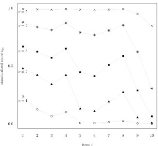
The normalized item scores for each latent state are plotted in Figure 1; see Table 1

for a summary description of each item. Patients in the first latent state experience some

difficulties and require some assistance related to the first four items: use of the shower

stall or bath tube, personal hygiene, and dressing the upper, and lower part of the body.

The need for assistance increases for individuals in the second latent state with respect

to the activities related to those items and some initial difficulties arise in transferring to

and using the WC, walking, and moving around. For patients in latent state 3, the needed

assistance become intensive for all activities apart from mobility in bed and eating. Latent

state 4 includes those requiring the assistance of two or more persons (apart from eating,

for which the assistance is limited). Finally, individuals in latent state 5 are totally unable

itemj

st

an

d

ar

d

iz

ed

sc

or

e

sj

v

v= 1

v= 2

v= 3

v= 4

v= 5

1 2 3 4 5 6 7 8 9 10

0.0 0.5 1.0

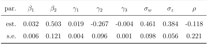
Turning the attention to the latent process, Table 3 contains estimates and standard

errors for the main parameters of the model with five latent states, once the covariate age

squared - that is not significant - has been removed. The coefficients ˆβ1 and ˆγ1 represent

the effect of patients’ age (in years) on their initial and transition probabilities respectively.

Given the assumed parametrization, it is not surprising to observe positive values,

meaning that older patients have initial and transition probabilities more concentrated on

the higher states, that is on the states associated to worse health conditions. It is also

interesting to examine the gender effect, expressed by ˆβ2 and ˆγ2. As gender is coded here

as a binary variable equal to 1 for females and 0 for males, from Table 3 we evince that

females are in a worse physical condition at the first occasion ( ˆβ2 > 0), whereas males

migrate towards critical health states with higher probability at the following occasions

(ˆγ2 < 0). Finally, the negative estimate ˆγ3 denotes that patients for which measurement

occasions are more distant have a lower tendency to move to worse states. This result

may be explained by nursing homes’ tendency to anticipate measurements when there is a

worsening in the health conditions of their patients (see Section 2). All these parameters

are significantly different from zero at 5% significance level. A significant effect of age on

initial probabilities, consistent with the one reported here, is found also by Bartolucci et al.

(2009), which focus on the period 2003-2005. However, their findings exclude a significant

par. β1 β2 γ1 γ2 γ3 σw σz ρ

est. 0.032 0.503 0.019 -0.267 -0.004 0.461 0.384 -0.118

s.e. 0.006 0.121 0.004 0.096 0.001 0.098 0.056 0.221

effect of gender on initial and transition probabilities as well as an effect of age on transition

probabilities.

The two random effect coefficients are ˆσw = 0.461 and ˆσz = 0.384, whereas the estimated

correlation is ˆρ = −0.118. Standard errors for these estimates are reported in Table 3, but statistical t-tests are performed on the parameter transformation scales mentioned in Section 3.3 to deal with parameters varying on the real line. Specifically, we have

log(ˆσw) = −0.774 (s.e. 0.212), log(ˆσz) = −0.957 (s.e. 0.146), and F(ˆρ) = −0.119 (s.e.

0.225). From these results we conclude that σw and σz are significantly greater than 0.25

(p-values 0.0019 and 0.0017 on the logarithmic scale), while ρ is not significantly different from zero (p-value 0.5972 on the Fisher transformation scale). The absence of correlation between the random effects permits to interpretZhas an NH performance measure. On the

contrary, a - say - positive correlation would imply that nursing homes with a more relevant

effect on transition towards critical health states are also more likely to host unhealthier

patients at the first occasion. In this case, a comparison between NHs based on the Zh

variables would not account for the different complexities nursing homes have to face at a

first stage.

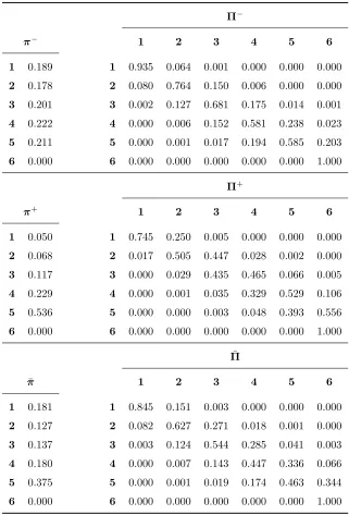
To understand the impact of these NH effects in terms of initial and transition

probabil-ities, in Table 4 we report the initial probability vectors and the 180-day ahead transition

matrices for the nursing homes with the higher and lower effects. Notice that these four

ar-rays are associated to four different NHs, that is, the nursing home with the higher (lower)

effect on initial probabilities is not the one with the higher (lower) effect on transition

prob-abilities. Lower effect initial and transition probabilities are denoted by π− _andΠ−_{, while}

higher effect ones by π+ and Π+. Each array is computed via the standard population method (Kitagawa, 1964), meaning that it is averaged across the same set of patients (and,

Π−

π− 1 2 3 4 5 6

1 _0.189 1 _{0.935 0.064 0.001 0.000 0.000 0.000} 2 _0.178 2 _{0.080 0.764 0.150 0.006 0.000 0.000} 3 _0.201 3 _{0.002 0.127 0.681 0.175 0.014 0.001} 4 _0.222 4 _{0.000 0.006 0.152 0.581 0.238 0.023} 5 _0.211 5 _{0.000 0.001 0.017 0.194 0.585 0.203} 6 _0.000 6 _{0.000 0.000 0.000 0.000 0.000 1.000}

Π+

π+ _{1 2 3 4 5 6}

1 _0.050 1 _{0.745 0.250 0.005 0.000 0.000 0.000} 2 _0.068 2 _{0.017 0.505 0.447 0.028 0.002 0.000} 3 _0.117 3 _{0.000 0.029 0.435 0.465 0.066 0.005} 4 _0.229 4 _{0.000 0.001 0.035 0.329 0.529 0.106} 5 _0.536 5 _{0.000 0.000 0.003 0.048 0.393 0.556} 6 _0.000 6 _{0.000 0.000 0.000 0.000 0.000 1.000}

¯

Π

¯

π 1 2 3 4 5 6

1 _0.181 1 _{0.845 0.151 0.003 0.000 0.000 0.000} 2 _0.127 2 _{0.082 0.627 0.271 0.018 0.001 0.000} 3 _0.137 3 _{0.003 0.124 0.544 0.285 0.041 0.003} 4 _0.180 4 _{0.000 0.007 0.143 0.447 0.336 0.066} 5 _0.375 5 _{0.000 0.001 0.019 0.174 0.463 0.344} 6 _0.000 6 _{0.000 0.000 0.000 0.000 0.000 1.000}

rule out the case-mix, which in this context is the effect of the different NH compositions

with regard to patients’ age and gender. The standard population is taken here to be the

available sample of patients, irrespective of the NH they belong to. Finally, the overall

averaged initial and transition probabilities, pooling together all NHs, denoted by ¯π and ¯

Π, are also reported in Table 4. We recall that latent state 6 corresponds to the additional

state associated to death, and many probabilities involving it are constrained to zero or

one as illustrated in Section 3.2.

Looking at the overall transition probabilities, it is worth to notice that the persistence

in the same state after a 180-day time period decreases for higher latent states. Beside

that, the probability of worsening is greater than the probability of improving the health

condition. The probability of death increases with the latent state and reaches 34.4% in

latent state 5.

As regards the NH effects on the transition probabilities, the largest effect yields the

lowest persistence probabilities and the greatest probabilities of death, especially in latent

state 5, compared to the least effect. In this respect we can produce a ranking of the NHs

with respect to their ability in avoiding the worsening of patients’ health conditions. To

this purpose, we can use the scaled posterior expectation

˜

Zh = ˆσzE(Zh|Xh =xh,Yh =yh), h= 1, . . . , H.

Given the model assumptions, this quantity can be obtained from the approximation

E(Uh|Xh =xh,Yh =yh)≈ Q

X

q=1

νqαhq

where

αhq =

P(Yh =yh|Xh =xh,Uh =νq)λq

PQ

q=1P(Yh =yh|Xh =xh,Uh =νq)λq

Nursing Homes

95%

O

v

er

lap

In

te

rv

al

s

0 1

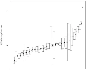
Figure 2: Posterior random effects for transition probabilities: caterpillar plot of 95%

Figure 2 depicts the caterpillar plot for the values of ˜Zh. The vertical bars are the

95% overlap intervals for pairwise comparisons: the effects on transition probabilities of

two nursing homes are significantly different at the 5% level if their intervals do not

over-lap (Goldstein and Healy, 1995). More than 60% of the pairwise comparisons are

signif-icantly different, denoting the importance of accounting for clustering in this application.

We recall that lower values of ˜Zh correspond to better NH performances. Notice that the

worst-performing NH, whose effect is pictured in the upper right-hand corner of Figure 2,

is the one with the higher number of patients (96). Obviously, the smaller the number of

units in the cluster, the larger the overlap interval.

5

Conclusions

In this work, we built a multilevel latent Markov model to evaluate the performance of a

group of nursing homes (NHs). We constructed a NH ranking based on the capability each

NH shows in improving or maintaining its patients in the best physical health conditions.

Health status was modeled like a categorical ordinal variable. As proxies of such a variable,

which is not directly observable, ten items measuring the so-called Activities of Daily Living

(ADL) were used. We applied our model to a longitudinal dataset collected in the Umbria

region (Italy) within the Long Term Care Facilities program, a public health protocol in

which patients in nursing homes are administered a questionnaire collecting information

also on the ADL. Results show that many pairwise differences between NH performances

are statistically significant.

NH effects were modeled by means of a continuous bivariate random effect, so that

the performance-based ranking can be obtained. Specifically, a normal distribution has

distribution may considerably affect the results, specific reasons to discard the normality

assumption do not appear to exist here. NH effects could in principle be estimated as fixed

effects by introducing binary variables in the regression equations (Bartolucci et al., 2009).

Within this framework, estimates are typically obtained via an Expectation Maximization

(EM) algorithm. This approach has the advantage of avoiding an untestable assumption

(that is, the specification of distributional form for random effects), but it is problematic

in the presence of small clusters, for which the estimation process might be unstable or

even unfeasible. For example, to obtain the EM estimates we used as starting point for the

multilevel model (see Section 3.3), we had to aggregate nursing homes with less than ten

patients.

Finally, it is worth to mention that alternative estimation methods were also proposed

within this framework. These include three-step estimation (Bartolucci et al., 2015) and

Bayesian estimation (Raffa and Dubin, 2015). Extending them to a multilevel context

would widen the range of possible estimation methods for this kind of data. Furthermore,

we argue that traditional tools to handle non-ignorable missingness - like joint models - are

still not widespread in the class of latent Markov models. In our view, these represent two

interesting lines of work future research in this area might be concerned with.

References

Altman, R. M. (2007). Mixed hidden Markov models: an extension of the hidden Markov

model to the longitudinal data setting. Journal of the American Statistical

Associa-tion 102(477), 201–210.

selection in the latent Markov model for longitudinal data. Advances in Data Analysis

and Classification 8(2), 125–145.

Bartolucci, F., A. Farcomeni, and F. Pennoni (2013). Latent Markov Models for

Longitu-dinal Data. Statistics in the Social and Behavioural Sciences. Chapman & Hall/CRC.

Bartolucci, F. and M. Lupparelli (2016). Pairwise likelihood inference for nested hidden

Markov chain models for multilevel longitudinal data.Journal of the American Statistical

Association 111(513), 216–228.

Bartolucci, F., M. Lupparelli, and G. E. Montanari (2009). Latent Markov model for

longitudinal binary data: an application to the performance evaluation of nursing homes.

The Annals of Applied Statistics 3(2), 611–636.

Bartolucci, F., G. E. Montanari, and S. Pandolfi (2015). Three-step estimation of latent

Markov models with covariates. Computational Statistics & Data Analysis 83, 287–301.

Bartolucci, F., F. Pennoni, and G. Vittadini (2011). Assessment of school performance

through a multilevel latent Markov Rasch model. Journal of Educational and Behavioral

Statistics 36(4), 491–522.

Baum, L. E., T. Petrie, G. Soules, and N. Weiss (1970). A maximization technique occurring

in the statistical analysis of probabilistic functions of Markov chains. The Annals of

Mathematical Statistics 41, 164–171.

Dempster, A. P., N. M. Laird, and D. B. Rubin (1977). Maximum likelihood from

incom-plete data via the EM algorithm.Journal of the Royal Statistical Society, Series B 39(1),

Fisher, R. A. (1915). Frequency distribution of the values of the correlation coefficient in

samples from an indefinitely large population. Biometrika 10(4), 507–521.

Fletcher, R. (1987). Practical methods of optimization (2nd ed.). New York: John Wiley

& Sons.

Gnaldi, M., S. Bacci, and F. Bartolucci (2016). A multilevel finite mixture item response

model to cluster examinees and schools. Advances in Data Analysis and

Classifica-tion 10(1), 53–70.

Goldstein, H. and M. J. R. Healy (1995). The graphical presentation of a collection of

means. Journal of the Royal Statistical Society, Series A 158(1), 175–177.

Goodman, L. A. (1974). Exploratory latent structure analysis using both identifiable and

unidentifiable models. Biometrika 61(2), 215–231.

Gray, A. (2009). Population aging and health care expenditure. China Labor

Eco-nomics 1(10), 105–114.

Henry, K. and B. Muth´en (2010). Multilevel latent class analysis: An application of

adoles-cent smoking typologies with individual and contextual predictors. Structural Equation

Modeling 17(2), 193–215.

Hirdes, J. P., G. Ljunggren, J. N. Morris, D. H. Frijters, H. Finne Soveri, L. Gray, M.

Bj¨ork-gren, and R. Gilgen (2008). Reliability of the interRAI suite of assessment instruments:

a 12-country study of an integrated health information system. BMC Health Services

Research 8(1), 277.

of the interRAI Long Term Care Facilities (LTCF) and interRAI Home Care (HC).

Geriatrics & Gerontology International 15(2), 220–228.

Kitagawa, E. M. (1964). Standardized comparisons in population research.

Demogra-phy 1(1), 296–315.

Koukounari, A., I. Moustaki, N. C. Grassly, I. M. Blake, M.-G. Bas´a˜nez, M. Gambhir, D. C.

Mabey, R. L. Bailey, M. J. Burton, and A. W. Solomon (2013). Using a nonparametric

multilevel latent Markov model to evaluate diagnostics for trachoma. American Journal

of Epidemiology 177(9), 913–922.

Little, R. J. and D. B. Rubin (2002). Statistical Analysis with Missing Data (2nd _ed.).

Wiley.

Makai, P., W. B. Brouwer, M. A. Koopmanschap, E. A. Stolk, and A. P. Nieboer (2014).

Quality of life instruments for economic evaluations in health and social care for older

people: a systematic review. Social Science & Medicine 102, 83–93.

Maruotti, A. (2011). Mixed hidden Markov models for longitudinal data: an overview.

International Statistical Review 79(3), 427–454.

Maruotti, A. and R. Rocci (2012). A mixed nonhomogeneous hidden Markov model for

categorical data, with application to alcohol consumption. Statistics in Medicine 31(9),

871–886.

Montanari, G. E. and S. Pandolfi (2016). Evaluation of health care services through a

latent Markov model with covariates. InSIS 2016 - 48th

Scientific Meeting of the Italian

Montanari, G. E., M. G. Ranalli, and P. Eusebi (2010). Multilevel latent class models for

evaluation of long-term care facilities. InData Analysis and Classification, pp. 249–256.

Springer.

Oehlert, G. W. (1992). A note on the delta method. The American Statistician 46(1),

27–29.

Press, W. H., B. P. Flannery, S. A. Teukolsky, and W. T. Vetterling (1989). Numerical

recipes, Volume 3. Cambridge University Press, Cambridge.

Raffa, J. D. and J. A. Dubin (2015). Multivariate longitudinal data analysis with mixed

effects hidden Markov models. Biometrics 71(3), 821–831.

Schwarz, G. (1978). Estimating the dimension of a model. The Annals of Statistics 6(2),

461–464.

Stephens, M. (2000). Dealing with label switching in mixture models. Journal of the Royal

Statistical Society, Series B 62(4), 795–809.

Vermunt, J. (2003). Multilevel latent class models. Sociological Methodology 33(1), 213–

239.

Vermunt, J. K., R. Langeheine, and U. Bockenholt (1999). Discrete-time discrete-state

latent Markov models with time-constant and time-varying covariates. Journal of

Edu-cational and Behavioral Statistics 24(2), 179–207.

Welch, L. R. (2003). Hidden Markov models and the Baum-Welch algorithm. IEEE

White, C. (2007). Health care spending growth: how different is the United States from

the rest of the OECD? Health Affairs 26(1), 154–161.

Wiggins, L. M. (1973). Panel analysis: Latent probability models for attitude and behavior

A multilevel latent Markov model for the

evaluation of nursing homes’ performance:

1

Log-likelihood gradient

The approximate gradient of the log-likelihood function is given by

∂ℓ(θ)

∂θ ≈

H

X

h=1

1

P(Yh =yh|Xh =xh) Q X q=1 " exp nh X i=1

ℓhiq(θ)

nh

X

i=1

∂ℓhiq(θ) ∂θ

λq

#

, (1)

where ℓhiq(θ) = logP(Yhi =yhi|Xhi=xhi,Uh =νq). Given the complete log-likelihood

ℓ∗

hiq(θ) = logP(Yhi=yhi,Vhi=vhi|Xhi =xhi,Uh =νq)

and its posterior expectation E∗

hiq(θ) = E(ℓ∗hiq(θ)|Yhi = yhi), a theoretical result (Oakes,

1999) stating that

∂ℓhiq(θ)

∂θ =

∂E∗ hiq(θ) ∂θ is exploited to compute each derivative present in (1).

2

Results for the model with

k

= 6

In this section, we report the results for the model with k = 6. As stated in the paper,

these are not substantially different from those obtained in the model withk = 5, denoting

the stability of the conclusions drawn. Table 1 reports estimates and standard errors for

the same parameters we consider in the model with five latent states. A comparison with

paper’s Table 3 shows that both estimates and standard errors are very similar in the two

models. Parameters’ significance and interpretation remain unchanged.

Figure 1 reports the normalized item scores. Again, the overall trend is very close

to that of the model with k = 5 (paper’s Figure 1). Specifically, once more we observe

that for every latent statev the biggest difficulties concern items 1 and 4 (washing/taking a

β1 β2 γ1 γ2 γ3 σw σz ρ

est. 0.032 0.482 0.020 -0.262 -0.004 0.469 0.372 -0.131

s.e. 0.006 0.121 0.004 0.095 0.001 0.102 0.056 0.220

Table 1: Main parameter estimates and standard errors for the model with k = 6

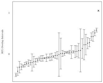
and eating (items 9 and 10). Figure 2 depicts the caterpillar plot of the scaled posterior

expectations ˜Zh. The resulting ranking is almost identical to the previous one, with a

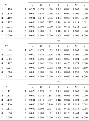
Spearman correlation coefficient of 0.995. Finally, Table 2 is the analogous for k = 6 of

paper’s Table 4. Once again, results are very similar overall.

References

Oakes, D. (1999). Direct calculation of the information matrix via the em. J. R. Stat. Soc.

itemj

st

an

d

ar

d

iz

ed

sc

or

e

sj

v

v= 1

v= 2

v= 3

v= 4

v= 5

v= 6

1 2 3 4 5 6 7 8 9 10

0.0 0.5 1.0

Nursing Homes

95%

O

v

er

lap

In

te

rv

al

s

0 1

Figure 2: Posterior random effects for transition probabilities: caterpillar plot of 95%

Π−

π− 1 2 3 4 5 6 7

1 _0.103 1 _{0.924 0.076 0.000 0.000 0.000 0.000 0.000}

2 _0.139 2 _{0.046 0.854 0.096 0.004 0.000 0.000 0.000}

3 _0.160 3 _{0.001 0.112 0.673 0.200 0.013 0.001 0.000}

4 _0.177 4 _{0.000 0.007 0.157 0.624 0.194 0.018 0.001}

5 _0.214 5 _{0.000 0.000 0.010 0.154 0.566 0.244 0.025}

6 _0.206 6 _{0.000 0.000 0.001 0.018 0.196 0.580 0.206}

7 _0.000 7 _{0.000 0.000 0.000 0.000 0.000 0.000 1.000}

Π+

π+ _{1 2 3 4 5 6 7}

1 _0.024 1 _{0.719 0.279 0.002 0.000 0.000 0.000 0.000}

2 _0.042 2 _{0.010 0.646 0.326 0.017 0.001 0.000 0.000}

3 _0.066 3 _{0.000 0.026 0.412 0.499 0.058 0.004 0.000}

4 _0.107 4 _{0.000 0.001 0.038 0.401 0.476 0.078 0.006}

5 _0.225 5 _{0.000 0.000 0.002 0.038 0.326 0.525 0.109}

6 _0.536 6 _{0.000 0.000 0.000 0.004 0.051 0.396 0.549}

7 _0.000 7 _{0.000 0.000 0.000 0.000 0.000 0.000 1.000}

¯

Π

¯

π 1 2 3 4 5 6 7

1 _0.111 1 _{0.829 0.170 0.001 0.000 0.000 0.000 0.000}

2 _0.111 2 _{0.049 0.742 0.198 0.011 0.001 0.000 0.000}

3 _0.110 3 _{0.001 0.110 0.537 0.312 0.037 0.003 0.000}

4 _0.120 4 _{0.000 0.007 0.146 0.496 0.297 0.049 0.004}

5 _0.174 5 _{0.000 0.000 0.011 0.143 0.439 0.339 0.068}

6 _0.373 6 _{0.000 0.000 0.001 0.020 0.173 0.463 0.343}

7 _0.000 7 _{0.000 0.000 0.000 0.000 0.000 0.000 1.000}

Table 2: Minimum effect, maximum effect and average initial and transition probabilities