Munich Personal RePEc Archive
Causality deficit-inflation: Wavelet
Transform
Elmrabet, Maissa and Boulila, Ghazi
13 December 2018
Causality deficit-inflation: Wavelet Transform
Elmrabet Maissa∗and Ghazi Boulila†
December 13, 2018
Abstract
Few researchers have addressed the problem of the causality inflation-deficits, and even Previous work treated this causality they have only focused on the Granger causality technique in which the results of this approach raises many doubts. This investigation aim to study the relationship between inflation and the pri-mary deficit using the wavelet transform for different euro area member countries from 1980 until 2014 with quarterly data. We have characterized the inflation-primary deficit relationship in a time-frequency scale. First we found that the deficit causes inflation in log term. We detected also, that inflation-primary deficit relationship is highly consistent during the post-financial crisis in the euro area in the long run. Finally we can judge through the wavelet transform that this relationship is non linear.
Keywords:deficit, inflation, wavelet.
1
Introduction
We bring down the curtain that, after the 2008 financial crisis, the inflation rate and debt ratio sharply increase. To that end, it will be substantive to shed light on these economic phenomena. Indeed, the primary balance is an important indicator of a State’s economic situation and gives a conspicuous idea of the unbounded evolution of public debt. Whilst copious theoretical studies have shown that primary deficits are inflationary Catao & Terrones (2005), Lin & Chu (2013). Notwithstanding, to date, no empirical study started the ball rolling concerning a statistically significant link between the deficit-inflation relationship in developed countries, albeit in developing countries, De Haan & Zelhorst (1990), Metin (1998),Domaç & Yücel (2005), have found a chief causality of budget deficits on inflation in high-inflation countries. Hence the importance of our research. In this investigation our objective is to study the relationship between inflation, and the primary deficit using the wavelet transform for different euro area member countries. We have characterized the primary inflation-deficit relationship in a time-frequency scale in an attempt to disentangle four conclusions. i) find out if there is a relationship between these target variables. ii) know if this causality is a long-term causality or a short-term causality. iii) know the intention of causality, i. e. if inflation causes the deficit or reciprocally. iv) know the type of causality, i. e. linear or non-linear causality. The originality of this research is to know what inflation and the primary deficit are dependent on before or after the 2008 financial crisis? Did inflation drive the deficit or reciprocally? And are euro area member countries converging or diverging? These findings have important implications for risk management, and for monetary policies to control inflationary pressures as well as the debt ratio. In this article to tackle our problem and answer all these questions, we will start in the first section with a literature review. The second section will present the wavelet approach and then we will finish with the results and the conclusion.
2
literature review
Manifold studies, have agitated the linkage between inflation and deficit. In their research Lin & Chu (2013) bring to pass that the budget deficit has a high strike on inflation in high inflation episodes and a low impact in low inflation episodes. The results intimate that fiscal consolidation would be the more efficacious in firming prices in the higher the inflation rate. According to Sargent et al. (1981) , it is true that in a monetarist economy, the money supply is exogenous and determined independently by the central bank to control inflation, but this control is limited. Putting it differently,Assuming that the monetary authority is controlled by the fiscal authority, this leads the latter to independently announce all current and future deficits, which leads to deficits with signorage and therefore the emergence of inflation. Against this background, it can be said that the deficit and inflation are dynamically correlated.Given the past theoretical research (Catao & Terrones (2005) Blanchard et al. (1989)), until today we can not conclude that there is a study that is interested in mentoring the exact relationship between inflation and deficit in spite of Kliem et al. (2016)’s recherche where he has studied the co-movement between these two target variables and who can only show that this relationship is non-linear. In fact, Kliem et al. (2016) studied the relationship between the government deficit and inflation using American data from 1900 to 2011 using the low-frequency approach of Lucas (1980) and Sargent and Surio (2011) to assess the low-frequency relationship of these two filtered time series (filtering inflation and deficit and deficit by the filter proposed by Lucas (1980)), allowing them to focus on the low-frequency variation. They found that any increase in the primary deficit leads to an increase in inflation. In this context, the empirical studies regarding the united states (Hamburger & Zwick (1981), Dwyer Jr (1982), Darrat (1985), Ahking & Miller (1985), King & Plosser (1985)) and those in others developed countries (King & Plosser (1985),Giannaros & Kolluri (1985),Protopapadakis & Siegel (1987), Barnhart & Darrat (1988)) could not find results that explain the relationship between these two target variables.for developing countries, most empirical studies can draw a conclusion on these two variables. indeed, during the period of high inflation, they find that there are significant causal effects between inflation and the budget deficit. (Metin (1998),De Haan & Zelhorst (1990) , Domaç & Yücel (2005) , and Lin & Chu (2013)). Since before, several studies have used different methodology to explain the relationship betwixt inflation and deficit.
From a theoretical point of view and taking into consideration the factors that can influence inflation Kaur (2018) focused on the empirical study. Indeed, in his work he tried to increase the investigation on the causality between money supply, exchange rates, budget deficit and inflation during the period 1970-1971 to 2014-2015 in India. To do this he used two techniques.The first is Granger causality to test short-term causality and the second is the Johansen’s co-integration technique to test the existence and effectiveness of several of the co-integration vectors . Kaur (2018) argued that there is a long-term relationship between budget deficit, money supply, exchange rate volatility and inflation, but he failed to provide adequate evidence to confirm the causality from budget deficit to inflation through Granger’s causality tests. One of the major drawbacks to adopting this technique (Granger causality ) is that fiscal theory of the price level is unable to find empirical support in the case of India. then, This is something of a pitfall if once accepts that the effectiveness of the budget deficit as an instrument for price stabilization in the short term. Vast amount of documentation on the relationship between budget deficits and inflation, using cross-sectional and panel data. Cutting edge paper of Karras (1994)tested the relationship using panel estimation. He claimed that deficits are not inflationary in 32 countries. Despite Cottarelli (1998) demonstrate a significant results concerning the impact of budget deficits on inflation in industrial economies and transition economies using the dynamic panel model.
low in countries with low-inflation and countries with high-inflation during low-inflation episodes. However this connection is strong only in high-inflation countries during high inflation episodes. Catao & Terrones (2005) They draw our attention to the impact of deficits on inflation and this influence is stronger either in high inflation or in developing countries. this empirically investigation using the group average estimation model, showed that, developing countries in which there is political instability, limited access to external borrowing, and less effective tax collection , have a propensity to have a higher inflation tax. is known about the regimes of "monetary dominance" and "fiscal dominance" examine the connection between inflation and budget deficits which are largely treated in the well-known article of Sargent and Wallace (1981). On the first hand, as we know, the the budget deficit is generated by the issuance of bonds as well as the seignorage created by the central bank whose monetary policy is independent. On the second hand, the State representing the budgetary authority faces a budgetary constraint imposed by the central bank, which in turn represents the monetary authority . in this case both the money supply and the budget deficit can be controlled by the central bank without inflation occurring. if not, if there is budgetary domination, then in these circumstances the central bank can not control neither money supply nor budget deficits because the latter lead to inflation in this case. There is still considerable ambiguity concerning the relationship between primary deficit and inflation. in this context. several experts found that the effect of primary deficit on inflation is negligible In a major advance in 1988, Barnhart and Darrat surveyed that the deficit don’t causes an increase in monetary growth and Reciprocally monetary growth don’t causes deficit. Giannaros and Kolluri (1986) has already noted a consistency with Barnhart and Darrat (1988) and claimed that the impact of budget deficits on money supply and inflation is insignificant for the data from 10 industrialized countries. The set up used by previous authors can be found with Komulainen & Pirttilä (2002) how use data from Russia, Bulgaria and Romania and find that the deficit does not play an inflationary role.However,Metin (1998)concludes that deficits causes directly inflation in Turkey during the period 1954-1986. Using the co-integration analysis. De Haan and Zelhorst (1990) underlines that there is no no evidence to affirm "the fiscal dominance hypothesis" and concluded that the correlation betwixt inflation and deficits are only in the high inflation periods. Using the coi-ntegration analysis, Also Loungani and Swagel (2003) comes to the conclusion that the fiscal balance is weakly correlated with inflation in 53 developing countries between 1964 and 1998, and in a high average inflation the correlation becomes stronger. add to that, they find a non-linear relationship between these tow variables,and when the deficit-to-GDP ratio is above 5 % the effect of deficits on inflation is significant.In the same reflection, that budget deficit has a significant impact on inflation in high inflation periods, the investigation of DomaÃ˘g and YÃijcel (2005) intervenes using a poled probit estimations in 15 emerging markets from 1980 to 2001.
3
Methodology : wavelet approach
The method that will be presented throughout this section is abundant in the field of electrical engineering to filter signals. The idea is to borrow all these techniques from the macroeconomic domain in order to study the behaviour of a non-stationary process in order to find results explaining whether there is a causality between the macroeconomic aggregates in question not only in a time domain but rather in a time-frequency-scale domain. To do this. Indeed, the choice of this technique is explained by economic intuition, whose knowledge of the behaviour of the series from a time-frequency point of view provides information on the nature of instabilities and the velocity of the bi-variance between inflation and the deficit.
Granger (1969). This notion, often referred to as the Granger causality, has been applied in many fields of study, such as finance and economics, signal processing, neuroscience, image processing, geophysics, etc. Despite Granger’s causality has succeeded in affirming whether there is really a relationship between the variables, it has limitations, first of all, regarding the causality of variance, the causality of risk, the causality of quantiles, the causality of the mean as well as the distribution. In addition to these limitations, this Granger causality method is unable to distinguish between long and short-term causal effects. Once causal effects are recorded and based on Granger causality, location in the frequency domain regardless of whether it is low (short term) or high frequency (long term) will be difficult. However, the causal relationship occurs over different hori-zons, which was developed in Geweke’s study (1982) to help us understand this difficulty. Indeed, Geweke (1982) innovative idea was to transform causality into a frequency domain. In this context Hosoya (2001), Breitung & Candelon (2006) and Yao & Hosoya (2000) align with Geweke (1982). At this stage the research studies have found that the frequency representation of the so-called”Fourrier transform” makes it possible to distinguish long-term causal effects from short-term causal effects, however, the fact that causality cannot be followed over time has caused limitations regarding”Granger-Geweke causality”, this has generated other innovative ideas such as”continuous wavelet transforms” to analyse time-frequency causality links Dhamala et al. (2008).Wavelet analysis has become widely used in empirical studies to understand the relationship be-tween variables and more precisely the temporal fluctuations bebe-tween them over different horizons. The ideas of Crowley (2007) , Yogo (2008), Dhamala et al (2008), Gallegati et al. (2011), Gençay et al. (2001), Fan & Gençay (2010) and Gallegati et al (2011) support this approach. However, what is more interesting in this chapter are the causal effects between the budget deficit and inflation. Indeed, the originality of this inves-tigation is reflected in the fact that it records how the causal effects between the deficit and inflation change over time and over time. Let’s look at the Fourrier transform (frequency representation), one of its advantages is that not only can long-term causal effects be isolated from short-term causal effects, but also it allows us to see if it is the short or long term that modulates the correlation between the variables. Unfortunately, the measurement of causal effects using the continuous wavelet transform was particularly problematic because such a measure only encompasses the amplitude between variables while the direction information needed to collect causal relationships is not available (see diagram). However, useful information about the delay rela-tionship (i.e. who starts first and causes who) is coded in the phase difference (or even phase circle). In few studies that are likely to undertake non-parametric wavelet causality (see Dhamala et al. 2008), the problem lies in calculating the spectral matrix factors in order to deduce the minimum phase. This process involves an inverse Fourier to communicate between the time domain and the frequency domain. At this stage, Owolabi et al. (2014) his study proposed an alternative method that abandons spectral matrix factorization but instead uses the information contained in both amplitude and phase difference to derive causal information between the variables of interest encoded in the phase difference. He authenticated the results based on this method by developing a data generation process (DGP) and found that the method is able to identify the causal period in synthetic data.
3.1 Causality of Geweke-Granger
To illustrate the two-variable (x and y) p-order VAR model is assumed as follows (Breitung and Candelon (2006), Dhamala et al (2008) or Olayeni (2015)):
With,Λ(L),Xtandǫtdenote respectively, the delay polynomial, the endogenous variables of target
vari-ables and the variance-covariance matrix error term notedΩwhich represents the mysterious part of the model. The matrix writing of the previous equation is given by :
"
I−Λxx(L) Λyx(L) Λxy(L) I−Λyy(L)
# × " xt yt # = " ǫx t
ǫyt
#
(2)
Ω =
"
Ωxx Ωyx Ωxy Ωyy
#
(3)
knowing thatΛ(L)is invertible, then we note its inverse byΘ(L)then we have :
Xt= Θ(L)ǫt (4)
The Fourier transform of the previous equation gives us:
X(ω) = Θ(ω)Ω ˜Θ(ω) (5)
With,X(ω)denotes the spectral power of variable X inω(it denotes the frequency);Θ(ω)denotes the transfer function between variables x and y andΘ(˜ ω)the conjugate (complex part) ofΘ(ω).
Θ(ω) =
"
Θxx(ω) Θyx(˜ ω) Θyx(ω) Θyy(ω)
#
(6)
Granger-Geweke causality in the frequency domain is given by:
Gy→x(ω) = log
"
Xxx(ω)
Xxx(ω)−
Ωxx−Ω2xy/Ωxx |Θxy(ω)|2
#
(7)
With, the numerator represents the spectral power of the variable x at the frequency ω and the denomi-nator presents the total power minus the causal contribution which represents the intrinsic power. Causality in the frequency domain allows us to reduce the time dimension to a single time point, resulting in a loss of information on time variation. However, the causality content in the frequency domain is interesting insofar as it informs us about fluctuations in causality in the time domain by decomposing the variables into different scales (frequency). This decomposition uses the transform into a Discrete Wavelet. This approach does not indicate the temporal content of causal effects. The extension of Granger-Geweke causality to non-parametric time-frequency domain modeling, as well as the analysis of the power distribution of Granger causality requires the factorized spectral matrix. The factorization of the spectral matrix is obtained through the use of Wilson’s algorithm (Wilson 1972). The necessary condition to factorize a spectral matrix is given by :
+π
Z
−π
If we noteΓthe minimum phase of the spectral density factor matrix phase :
Γ =
∞
X
t=0
Λtexp (−2iπωt) (9)
Thus, if we note byΩandΘrespectively the noise variance-covariance matrix and the minimum phase of the spectral transfer function :
Ω = Λ0ΛT0
Θ = ΓΛ−1 0
(10)
Then, the minimum phase of the spectral density factor matrix phase can be rewritten as follows:
Γ = ΘΣΘH (11)
With,ΘH transposed it from the Hermitian matrixΘ. The factorization of the matrixX(ω)is given by :
X= Γ˜Γ (12)
With,Γ˜ refers to the complex conjugate of the transposedΓ.
3.2 Causality in the Geweke-Granger sense proposed by Dhamala et al (2008)
The calculation of the spectral matrix and the minimum phase transfer function allow us to evaluate the Geweke-Granger time-frequency causality presented by equation (13) However, the calculation of the transfer function requires the determination of the spectral matrix and the convergence of the Wilson algorithm “La factorisation des densitÃl’s spectrales matricielles” (n.d.) which have disadvantages of this approach. These disadvantages are addressed by Dhamala et al (2008), who introduced the Wavelet transformation to the Geweke-Granger analysis. The new causality formula is parallel to the formula presented in the equation (7) in the following form:
Gy→x(s, τ) = log
h Wxx(s, τ)
Wxx(ω, τ)−
Ωxx−Ω2
xy/Ωxx |Θxy(s, τ)|2
i
(13)
With,Wxx(ω, τ)indicates the spectral power in Wavelet.
3.2.1 wavelet transform
The wavelet is a function defined on (L2(
R)), noted (ψ(t)).It must check the following analytical prop-erties such as mean and integral equal to zero and normalized :
+∞ R −∞
ψ(t) dt = 0
+∞
R
−∞
|ψ(t)|2
dt <0
In addition to the continuity that has been verified in the properties explained above, the wavelet must also satisfy the following admissibility status:
+∞
Z
−∞
|Ψ(t)|2
|ω| dω <∞ (15)
where, (Ψ(t)) is considered by the Fourier transform of (ψ(t)).
The projection of a series (x(t)) through a mother wavelet function is given by the following complex coefficients:
W(s, τ) =
+∞
Z
−∞
x(t)ψ∗
s,τ(t) dt (16)
with,
ψ∗
s,τ(t) = 1
p |s|ψ(
t−τ
s ) (17)
Where (x(t)) and (ψ∗
s,τ(t)) denote, respectively, a series and the atom of the mother wavelet transform. We
note by (s) a scale parameter (dilation) (s∈R∗+)and by (τ)a time location parameter (translation)(τ ∈R).
Translation and expansion allow us to determine the atoms of the wavelet. Dilation is a time shift, while translation is a time location,Translation and expansion allow us to determine the atoms of the wavelet. Dilation is a time shift, while translation is a time location Torrence & Compo (1998) have shown that it is possible to reconstruct the signal through the following formula:
x(t) = 1
C
+∞
Z
s=−∞
+∞
Z
τ=−∞
1
|s|2W(s, τ)ψs,τ(t) dsdτ (18)
3.3 The Geweke-Granger causality proposed by Rua (2013) and Olayeni (2015)
Rua (2013) proposed a measure of the correlation by the Continuous Wavelet Transform noted(ρxy(s,τ))1
given by:
ρxy(s, τ) = γ
s−1|ℜWm xy(s, τ)|
γns−1p |Wm
x (s, τ)|2
o
γns−1q|Wm y (s, τ)|2
o (19)
withγdesignates a time-scale smoothing operator. The correlation by the Continuous Wavelet Transform differs from the Wavelet Coherence noted(Rxy(s, τ))2, which is given by
Rxy(s, τ) =
γ
s−1
|Wm xy(s, τ)|
γns−1p |Wm
x (s, τ)|2
o
γns−1q|Wm y (s, τ)|2
o (20)
However, the analysis proposed by Rua (2013) shows these limitations insofar as it does not integrate informa-tion on the direcinforma-tion between the variables. Olayeni (2015) proposed a modificainforma-tion on the correlainforma-tion of Rua (2013) by integrating the concept of phase difference between the variables. He proposed an indicator function (see equation...) that takes the value one if the variables are in phase and the value zero if not while basing
1
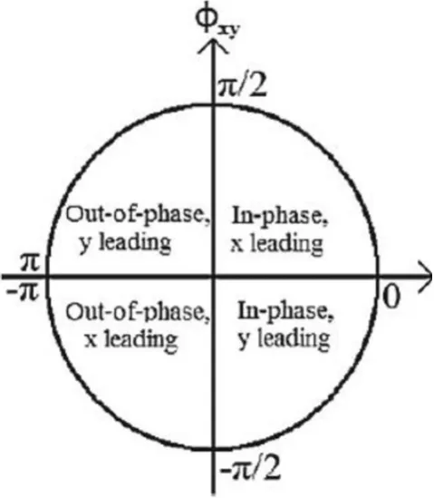
their analysis on the phase difference circle proposed by Aguira-Conraria and Soares (2011) (see figure 1). The concept of phase difference between two variables x and y is given by :
Φxy(s, τ) = Φx(s, τ)−Φy(s, τ) (21)
with,−π ≤Φxy ≤π.
The interval[−π, π]can be divided into four intervals, as indicated (see Table 1 figure ??):
• If Φxy ∈ [0, π/2],[−π/2,0] : the two variables are in phase, they are moving in the same direction (direction). We say that x leads to y, i. e. there is predictable information on x in the sense of Granger whenΦxy[0, π/2]and vice versa.
• IfΦxy ∈[π/2, π],[−π,−π/2]: the two variables are anti-phase, they move in the opposite direction. It
is said that y leads to x, i. e. x has predictable information about y whenΦxy ∈[π/2, π]and vice versa.
[image:9.595.179.419.295.570.2]Figure 1: Phase difference circle Conraria & Soares (2011)
Table 1: The lead-lag relationship
x leads y y leads x
In-phase Φxy(s, τ)∈(0, π/2) Φxy(s, τ)∈(−π/2,0)
Out-of-phase Φxy(s, τ)∈(−π,−π/2) Φxy(s, τ)∈(π/2, π)
Total phase Φxy(s, τ)∈(0, π/2)∪(−π,−π/2) Φxy(s, τ)∈(−π/2,0)∪(π/2, π)
Iy→x(s, τ) =
1, siΦxy(s, τ)∈J
With,Φxy(s, τ)denote the phase difference function :
Φxy(s, τ) = tan−1
ℑnWm xy(s, τ)
o
ℜnWm xy(s, τ)
o !
(23)
And J denotes intervals : [0,π
2],[−π,− π
2], and [0, π
2]∪[−π,− π 2],
4
Data
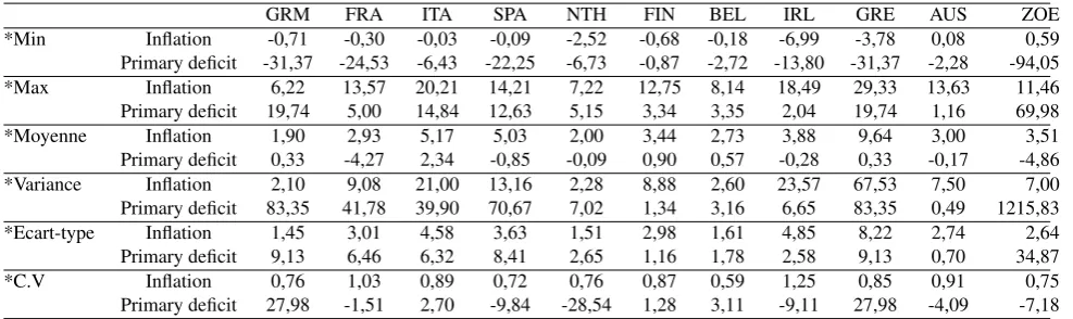
[image:10.595.55.549.504.651.2]We have built a quarterly database associated with the different macroeconomic variables. The various data are collected from data Stream. Indeed, this database of quarterly variables covers the period from 1980Q1 to 2014Q4 in the euro area. In our investigation we selected 10 countries from the area in addition to the euro area as classified into two categories: core countries (Germany, France, Austria, the Netherlands, Belgium, and Finland), and peripheral countries (Greece, Ireland, Spain, Italy). In our estimate we considered three main variables such as inflation, primary deficit and economic growth in order to study the relationship between in-flation and deficit while considering the economic growth of the area. Based on the article by?, inflation(π)is measured as the first annual differences in the logarithmic GDP deflator, where data are taken from the Oxford Economics database (Price Deflator, Gross Domestic Product, Index, 2010 =100). Oxford Economics defines inflation as a measure that tracks the price of all goods and services in a net of tax recovery. This measure dif-fers from the consumer price index, which is taxed on goods and services purchased by households, including indirect taxes. Regarding the primary deficit (d) it was measured by the variable ’ general government primary balance, euro ’ from the Oxford Economics database in Billions of euros at constant price which was defined by central and local government revenues less expenditure, excluding the payment of interest on consolidated government liabilities expressed in local currency. If the balance is negative, then the primary deficit is negative.
Table 2: Descriptive Statistics
GRM FRA ITA SPA NTH FIN BEL IRL GRE AUS ZOE *Min Inflation -0,71 -0,30 -0,03 -0,09 -2,52 -0,68 -0,18 -6,99 -3,78 0,08 0,59 Primary deficit -31,37 -24,53 -6,43 -22,25 -6,73 -0,87 -2,72 -13,80 -31,37 -2,28 -94,05 *Max Inflation 6,22 13,57 20,21 14,21 7,22 12,75 8,14 18,49 29,33 13,63 11,46 Primary deficit 19,74 5,00 14,84 12,63 5,15 3,34 3,35 2,04 19,74 1,16 69,98 *Moyenne Inflation 1,90 2,93 5,17 5,03 2,00 3,44 2,73 3,88 9,64 3,00 3,51 Primary deficit 0,33 -4,27 2,34 -0,85 -0,09 0,90 0,57 -0,28 0,33 -0,17 -4,86 *Variance Inflation 2,10 9,08 21,00 13,16 2,28 8,88 2,60 23,57 67,53 7,50 7,00 Primary deficit 83,35 41,78 39,90 70,67 7,02 1,34 3,16 6,65 83,35 0,49 1215,83 *Ecart-type Inflation 1,45 3,01 4,58 3,63 1,51 2,98 1,61 4,85 8,22 2,74 2,64 Primary deficit 9,13 6,46 6,32 8,41 2,65 1,16 1,78 2,58 9,13 0,70 34,87 *C.V Inflation 0,76 1,03 0,89 0,72 0,76 0,87 0,59 1,25 0,85 0,91 0,75 Primary deficit 27,98 -1,51 2,70 -9,84 -28,54 1,28 3,11 -9,11 27,98 -4,09 -7,18
3CV ( ariation Coefficient v= Moyenne/Ecart-type)
5
Results
In our study we will focus on the types of causality (linear or non-linear causality) for this reason we will interpret coherence by transforming it into a wavelet. When(Rxy(s, τ) = 1), therefore we can conclude that
(a) FINLAND (b) france
(c) GRECE (d) GERMANY
(e) IRLAND (f) GRECE
(g) NTHERLAND (h) SPAIN
[image:11.595.90.507.47.591.2](i) ZONE EURO
Figure 2: Wavelet Transform Coherence
olor (shows type of causality).The degradation of the blue colour means that the causality between inflation and the primary deficit is non-linear(Rxy(s, τ) = 0)and that the dependence between these two variables is
Austria : In the short term: it can be seen that there is a high dependence between inflation and the deficit (2004-2005). This causal relationship is linear during this same period. Indeed, this year we see that the primary deficit caused inflation in the short term. However, inflation-deficit consistency is low and non-linear between (1981-2003) and (2006-2014). Long-term: throughout the period it has been noted that there is a low dependence between inflation and deficit and throughout the same period have a non-linear relationship.
Germany : It should be noted that the Berlin Wall crisis (1991) had a negative impact on the country’s economic situation, particularly in terms of inflation. These effects spread until (1995-2000). There is a strong interdependence in the scalogram during this short term to medium term period. In the long term, it can be seen that before the 2008 financial crisis, there was little consistency between the deficit and inflation. This consistency is accentuated from 2008 onwards, when it can be seen that the two variables in question are in antiphase (arrow upwards, so inflation is ahead of the deficit). Concerning the type of causality, we note that in LT the causality between inflation and deficit, until 2011, is non-linear and then becomes linear.
France : In the short term: The wavelet transformed coherence scalogram shows that the inflation-primary
deficit relationship is highly consistent over the periods (1980-1981), (1993-1994), (2009-2011). Economically speaking, there is a dependency relationship between the variables, i.e. inflation drives the primary deficit in France during this short term period. In the long term: it can be seen that there is no interdependence between inflation and the primary deficit before the financial crisis (blue colour). The blue color also shows us that the causality between these two variables is non-linear in this period and then becomes linear beyond 2008. After the financial crisis, a strong coherence between the variables in question appears (yellow colour). According to our results, we can conclude that in the long term inflation leads to the primary deficit after the 2008 crisis in France.
Ireland : In the short term: there is a dependency relationship between inflation and the primary deficit
during the period 1980- 1982. Indeed, according to the scalogram, it can be concluded that during this period inflation led to the primary deficit in Ireland. This causality is therefore of a linear type (yellow colour). This interdependence during this period is explained by the Irish hunger strike in 1981. However, beyond 1983 there is little coherence between these two variables (a non-linear relationship). In the long term: from the 2008 financial crisis onwards, the coherence between inflation and the primary deficit is beginning to become increasingly strong. This causality is of a linear type. Whereas before 2008 the causality was non-linear. Indeed, according to the chart, inflation generates the primary deficit at both CT and LT during the period (1981-1982) and (2008-2014) respectively. This strong coherence is expressed by the subprime crisis and then by the 2010 eurozone debt crisis (the colour has become increasingly warm).
Greece : In the long term: throughout the period up to the financial crisis, there is little consistency between inflation and the deficit (blue colour). This coherence this coherence this coherence is accentuated only slightly after the financial crisis and from 2010 the coherence has become slightly strong (green color). Economically speaking, these results can be interpreted as follows: from the financial crisis onwards, the deficit has a slight influence on inflation (right arrow with green colour). But from the Greek debt crisis of 2010 the influence of the primary deficit on inflation becomes more noticeable. The causal relationship between these two variables is non-linear from 1981 to 2008.
Spain : In the long term, Spain’s result does not differ too much from the other results of the other euro
financial crisis. It can therefore be concluded that inflation leads the deficit in the long term after the subprime crisis
6
Conclusion
References
Ahking, F. W., & Miller, S. M. (1985). The relationship between government deficits, money growthm and inflation. Journal of macroeconomics,7(4), 447–467.
Barnhart, S. W., & Darrat, A. F. (1988). Budget deficits, money growth and causality: Further oecd evidence.
Journal of International Money and Finance,7(2), 231–242.
Blanchard, O. J., Fischer, S., BLANCHARD, O. A., et al. (1989). Lectures on macroeconomics. MIT press.
Breitung, J., & Candelon, B. (2006). Testing for short-and long-run causality: A frequency-domain approach.
Journal of Econometrics,132(2), 363–378.
Catao, L. A., & Terrones, M. E. (2005). Fiscal deficits and inflation. Journal of Monetary Economics,52(3), 529–554.
Conraria, L. A., & Soares, M. J. (2011). The continuous wavelet transform: A primer. NIPE Working Paper,
16, 1–43.
Cottarelli, M. C. (1998). The nonmonetary determinants of inflation: A panel data study. International Monetary Fund.
Crowley, P. M. (2007). A guide to wavelets for economists. Journal of Economic Surveys,21(2), 207–267.
Darrat, A. F. (1985). Inflation and federal budget deficits: some empirical results. Public Finance Quarterly,
13(2), 206–215.
De Haan, J., & Zelhorst, D. (1990). The impact of government deficits on money growth in developing countries. Journal of International Money and Finance,9(4), 455–469.
Dhamala, M., Rangarajan, G., & Ding, M. (2008). Estimating granger causality from fourier and wavelet transforms of time series data. Physical review letters,100(1), 018701.
Domaç, I., & Yücel, E. M. (2005). What triggers inflation in emerging market economies? Review of world economics,141(1), 141–164.
Dwyer Jr, G. P. (1982). Inflation and government deficits. Economic Inquiry,20(3), 315–329.
Fan, Y., & Gençay, R. (2010). Unit root tests with wavelets. Econometric Theory,26(5), 1305–1331.
Fischer, S., Sahay, R., & Végh, C. A. (2002). Modern hyper-and high inflations.Journal of Economic literature,
40(3), 837–880.
Gallegati, M., Gallegati, M., Ramsey, J. B., & Semmler, W. (2011). The us wage phillips curve across frequen-cies and over time. Oxford Bulletin of Economics and Statistics,73(4), 489–508.
Gençay, R., Selçuk, F., & Whitcher, B. J. (2001). An introduction to wavelets and other filtering methods in finance and economics. Elsevier.
Geweke, J. (1982). Measurement of linear dependence and feedback between multiple time series. Journal of the American statistical association,77(378), 304–313.
Granger, C. W. (1969). Investigating causal relations by econometric models and cross-spectral methods.
Econometrica: Journal of the Econometric Society, 424–438.
Hamburger, M. J., & Zwick, B. (1981). Deficits, money and inflation. Journal of Monetary Economics,7(1), 141–150.
Hosoya, Y. (2001). Elimination of third-series effect and defining partial measures of causality.Journal of time series analysis,22(5), 537–554.
Karras, G. (1994). Macroeconomic effects of budget deficits: further international evidence. Journal of International Money and Finance,13(2), 190–210.
Kaur, G. (2018). The relationship between fiscal deficit and inflation in india: A cointegration analysis.Journal of Business Thought,8, 42–70.
King, R. G., & Plosser, C. I. (1985). Money, deficits, and inflation. InCarnegie-rochester conference series on public policy(Vol. 22, pp. 147–195).
Kliem, M., Kriwoluzky, A., & Sarferaz, S. (2016). On the low-frequency relationship between public deficits and inflation. Journal of applied econometrics,31(3), 566–583.
Komulainen, T., & Pirttilä, J. (2002). Fiscal explanations for inflation: Any evidence from transition economies? Economics of Planning,35(3), 293–316.
La factorisation des densitÃl’s spectrales matricielles. (n.d.). Journal SIAM de mathÃl’matiques appliquÃl’es,
23, 420–426.
Lin, H.-Y., & Chu, H.-P. (2013). Are fiscal deficits inflationary? Journal of International Money and Finance,
32, 214–233.
Metin, K. (1998). The relationship between inflation and the budget deficit in turkey. Journal of Business & Economic Statistics,16(4), 412–422.
Owolabi, J., Amusan, L., Oloke, C. O., Olusanya, O., Tunji-Olayeni, P., Dele, O., . . . Omuh, I. (2014). Causes and effect of delay on project construction delivery time. International journal of education and research,
2(4), 197–208.
Protopapadakis, A. A., & Siegel, J. J. (1987). Are money growth and inflation related to government deficits? evidence from ten industrialized economies. Journal of International Money and Finance,6(1), 31–48.
Sargent, T. J., Wallace, N., et al. (1981). Some unpleasant monetarist arithmetic. Federal reserve bank of minneapolis quarterly review,5(3), 1–17.
Torrence, C., & Compo, G. P. (1998). A practical guide to wavelet analysis. Bulletin of the American Meteo-rological society,79(1), 61–78.
Yao, F., & Hosoya, Y. (2000). Inference on one-way effect and evidence in japanese macroeconomic data.
Journal of Econometrics,98(2), 225–255.
Yogo, M. (2008). Measuring business cycles: A wavelet analysis of economic time series. Economics Letters,