Load Density Analysis of Mobile Zigbee Coordinator in Hexagonal Configuration

Load Density Analysis of Mobile Zigbee Coordinator in

Hexagonal Configuration

S. R. Ramyah Anna University, Chennai, India

Email: [email protected]

Received December 18, 2011; revised January 21, 2012; accepted February 12, 2012

ABSTRACT

Mobility is one of the major new paradigms of the current Internet, and this is driving most of the research activity in networking throughout the World. The Mobility of Wireless Sensor Networks (WSN) has become a hot research theme in recent years due to its wide range of applications ranging from medical research to military. The widely adopted standard for wireless sensor network platform is IEEE 802.15.4/ZigBee. The IEEE 802.15.4/ZigBee is considered the “technology of choice” due to low-power, cost-effective communication and the reliability they provide. In this paper, we perform extensive network evaluation, to study the Effect of coordinator mobility on ZigBee mesh network, using OPNET Modeler. In mobile coordinator, the type of the trajectory along with the node density and the traffic are the major factors that decide the system performance. The results obtained from the wide analysis of ZigBee mesh network shows variation when the routers are placed at Hexagonal configuration with a mobile coordinator. In this paper, varia- tions in load metric is analyzed in hexagonal configuration by enabling and disabling ACK. Thus the status of ACK also plays a critical role in analysing load metrics.

Keywords: Zigbee; Mobile Coordinator; Load

1. Introduction

Recent research has intensively focused on the next gen-eration communication systems that aim to meet the in-creasing demand for services with higher data rates and enhanced service quality. The idea behind this simulation model was triggered by the need to build a very reliable model of the IEEE 802.15.4/ZigBee protocols for WSNs. The wireless sensor network architecture consists of a large number of wireless sensor nodes. The wireless sensor nodes are miniature battery powered devices with very less power consumption rates making them appropriate for use in the remote areas. These sensor nodes are dis- tributed randomly. A sensor can act as a Full Functional Device (FFD) or a Reduced Functional Device (RFD) [1], with at least one FFD acting as a Coordinator. The pri-mary goal of the RFDs (end devices) is to gather the data from the surrounding environment and route it to the coordinator which has superior computing capabilities and serves as gateway for the entire network.

Wireless networks have historically considered sup-port for mobile elements as an extra overhead. However, recent research has provided means by which network can take advantage of mobile elements. Particularly, in the case of wireless networks, mobile elements are delib-erately built into the system to improve the lifetime of the network, and act as mechanical carriers of data.

A number of researchers have proposed mobility as a solution to this problem of data gathering. Mobile ele-ments traversing the network can collect data from sen-sor nodes when they come near it. Existing mobility in the environment can be used [2-4] or mobile elements can be added to the system, which have the luxury to be recharged. This naturally avoids multi-hop and removes the relaying overhead of nodes near the base station. Various types of mobility have been considered for the mobile element. These can be broadly classified as ran-dom, predictable or controlled. Random-walk mobility is assumed to be independent of the network topology, traf-fic flows and residual energy of nodes [2]. The predict-able or fixed trajectory of a mobile sink is fully determi-nistic as the sink always follows the same path through the network. In some cases, the path actually selected is, in fact, enforced by artificial or natural obstacles in the environment. In the case of controlled mobility, the path of the sink becomes a function of the current state of network flows and nodes’ energy consumption, and it keeps adjusting itself to ensure optimal network perfor- mance at all times.

But none of them concentrated on the effect of the node density due to the mobility of the coordinator. The goal of this paper is to study the analysis of mobility of coor-dinator on the Load of the network.

This paper is organized as: Section 2 gives a brief overview of the IEEE 802.15.4 and the reason for adopt-ing Zigbee, Section III discusses about OPNET modeler, Section IV explains about the types of ZigBee devices and their network topologies, Section 5 describes the arrangement of nodes in the network and the trajectories for the coordinator motion, Section 6 gives the assump-tion and layout of network field, Secassump-tion 7 analyses the simulations performed using OPNET modeler and Sec-tion 8 concludes the paper giving the results.

2. Overview of IEEE 802.15.4 (Zigbee)

ZigBee takes its name from the zigzag flying of bees that forms a mesh network among flowers. It is an individu-ally simple organism that works together to tackle com-plex tasks. Zigbee (IEEE 802.15.4) standard intercon-nects simple, low power and low processing capability wireless devices. The Zigbee devices facilitate numerous applications such as pervasive computing, national secu-rity, monitoring and control etc. In recent years, the technology has been gaining use in industrial and com-mercial acceptance, this is clear from the wide spread use in defence, monitoring and control, commercial use etc.

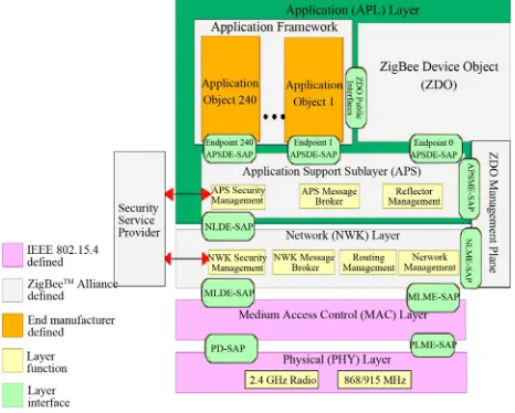
As shown in Figure 1 Zigbee architecture comprises of 4 layers—Physical Layer, MAC Layer, Network and Security Layer and Application Layer. Physical and MAC Layer are defined as IEEE 802.15.4 standards while the higher layers follow standards set by Zigbee Alliance. Our simulation model implements the physical layer of the IEEE 802.15.4 standard running at 2.4 GHz Frequency band with 250 kbps data rate. The MAC layer supports the beacon-enabled mode and implements slotted

Figure 1. Zigbee architecture.

CSMA/CA and GTS mechanism according to the stan-dard specification. There is also a battery module that computes the consumed and remaining energy levels. The network layer implements hierarchical tree routing according to the ZigBee standard. The application layer can generate best effort and/or real-time unacknowledged and/or acknowledged frames transmitted during Conten-tion Access Period (CAP) or ContenConten-tion Free Period (CFP) (contains GTSs) of the super frame, respectively.

3. Overview of OPNET

The OPNET Modeler environment includes tools for all phases of a study, including model design, simulation, data collection, and data analysis. OPNET Modeler pro- vides a comprehensive development environment sup- porting the modelling of communication networks and distributed systems. Both behaviour and performance of a model can be analysed by performing discrete event simulations [10]. A Graphical User Interface (GUI) sup-ports the configuration of the scenarios and the develop-ment of network models.

According to our personal experience, we strongly be-lieve that the current version of the WPAN implementa-tion in the network simulator (ns-2) simulator is not ac-curate for the simulation of wireless sensor networks. OPNET simulation model implements more accurately the IEEE 802.15.4/ZigBee protocols without these un-necessary overheads. This is mainly due to the amount of additional overheads introduced by the ns-2 simulator, since it imposes the use of a UDP (User Datagram Pro-tocol) agent in each node for generating data, and also the generation of ARP (Address Resolution Protocol) frames.

Three hierarchical levels for configuration are differ-entiated: Network level, Node level and Process level. Network level creating the topology of the network under investigation, Node level defining the behaviour of the node and controlling the flow of data between different functional elements inside the node and Process level describing the underlying protocols, represented by finite state machines (FSMs) and are created with states and transitions between states. The source code is based on C/C++.

4. Network Topologies in Zigbee

which route the data from the source to the destination. A router is able to pass on messages in a network, and is also able to have child nodes connect to it, whether it be another router, or an end device. These devices route the data as well as sense the data from their surrounding en-vironment. ZigBee end-devices are devices with least computing capabilities. The power saving features of a ZigBee network can be mainly credited to the end de-vices. Because these nodes are not used for routing traf-fic, they can be sleeping for the majority of the time, ex-panding battery life of such devices.

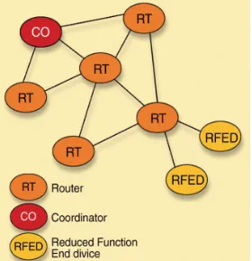
The ZigBee standard also defines 3 possible types of network Topology [1]: star, cluster-tree and peer-to-peer (mesh). In the star topology, direct communication link is established between devices and a single central control-ler, called the PAN coordinator. In cluster-tree topology, there is a parent child relationship between the nodes. Each node passes its packet to this parent and it then passes it further. In mesh topology, each device not only transmits to its parent but also to all the neighbouring de-vices as long as they are in range. It works on a proactive routing mechanism in which each node broadcasts a mes-sage and finds the shortest path on the basis of the replies from the routers. It is better than other topologies due to its powerful routing mechanism. Mesh topology supports “multi-hop” communications, through which data is passed by hopping from device to device using the most reliable communication links and the most cost-effective path until its destination is reached. The multi-hop ability also helps to provide fault tolerance, in that if one device fails or experiences interference, the network can reroute itself using the remaining devices (Figure 2).

Mesh networking is a powerful way to route data. Range is extended by allowing data to hop node to node and reliability is increased by “self healing” the ability to create alternate paths when one node fails or a connec-tion is lost. One popular mesh networking protocol is ZigBee, which is specifically designed for low-data rate, low-power applications. Zigbee Mesh networking has the following benefits:

Figure 2. Zigbee network mesh topology.

 Flexibility:The physical placement of a wireless mesh device is extremely flexible—as long as it is within communications range of other devices within the network, it can be placed nearly anywhere. Areas that would be difficult, expensive, or even impossible to cover within a wired network are accessible within wireless networks.

 Cost: Wireless removes the expense and time in-volved in installing and maintaining dedicated wiring to each device within the network.

 Scalability:A single mesh network can support thou-sands of individual devices. Adding new devices can be as simple as putting the device where you want it, and then turning it on.

 Reliability and robustness: A mesh network can be improved in many ways by adding more devices— extending distance, adding redundancy, and improv-ing link quality and the general reliability(Figure 3).

5. Router Configuration and Coordinator

Path

5.1. Arrangement of Routers

To avoid the deviation in the results due to random arran- gement of routers, two specific router configurations are used.

1) Square Configuration:In this configuration, routers are arranged on the corners of a network field. The posi-tion of routers is such as to cover the entire network field. The routers are not in the radio range of each other.

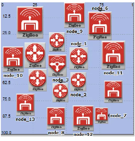
2) Hexagonal Configuration: In this configuration, routers are arranged so as to cover the entire network field and forming a hexagon. The vertices of the hexagon represent the routers. The routers are within the radio range of two adjacent routers. It is shown in Figure4.

From previous projects results, the Hexagonal con-figuration provide best results than Square concon-figuration.

Figure 4. Hexagonal configuration.

5.2. Coordinator Path Model

There are two different sink mobility models—random sink mobility model and fixed sink mobility model [11].

1) Random Sink Mobility Model: In this model the tra-jectory of the sink movement comprises of the random Sequence of segments distributed through the network.

2) Fixed Sink Mobility Model: In this model, the tra-jectory of the sink movement is along a fixed path, and during the entire simulation duration the sink keeps on moving on the same path.

Since we take mobile coordinator we set the trajectory as a Random mobility model.

6. Network Field Layout

The network setup consists of a network field within which the end devices are present, which sense the data and transmit via the routers (or directly) to the coordina-tor (sink).

 The network field is a square shaped region.

 The end-devices are distributed in a complete random manner.

 The routers are arranged in Hexagonal configuration.  The coordinator is mobile and it takes random path.  The impact of external interferences is considered zero.

The network layout can be shown in Figure 5.

7. ZigBee Simulation Using OPNET

7.1. Simulation Parameters

The simulations analysed in this section are performed on the OPNET Modeler v 14.5 [10]. ZigBee performs route discovery to determine the optimal path for mes-sages to take to its destination. This section will discuss then analysis various cases simulated on OPNET. The network field is of size 100 m × 100 m. The simulations are performed with 10, 20, 30, 40, and 50 end-devices. The topology used is Peer-to-Peer (Mesh) Topology. In the simulation, the distribution of end-devices is random.

Figure 5. Network layout.

The coordinator moves at a constant speed of 10 m/sec. The overall simulation time is 3600 sec with the meas-urements taken been aggregated at every 36 sec.

Table 1 shows the various network parameters and pa- rameter values used during simulation.

7.2. Number of Nodes

In this section, we change number of nodes and number of flows (keeping same flow/node ratio) and find out effect of number of nodes for load with and without ACK. Number of Nodes definitely affects for PAN bridge performance. Bridge node should be the bottle-neck node and performance degrades as the number of nodes increases. As number of nodes increases, number of flows also increases because flow/node ratio is fixed. More flows make more congestion, therefore delay in-creases.

Every node is explicitly defined as FFD or RFD, with higher energy levels for FFD nodes.

 For the ease of routing, it is assumed that each and Every node is location aware node with respect to the Base Station.

 Depending on the distance of the node from the Base Station and its radio range, a node calculate Number of hops required to connect to BS in terms of NET-WORK DEPTH.

7.3. Analysis of Simulation

In the analysis we will consider the load for different node density and the effect of ACK on load in a Hex-agonal Configuration of Routers.

Table 1. Simulation parameters.

Network Parameter Parameter Value

Transmission Range 60 m

Packet Size 1024 bits

GTS Disabled

Acknowledge wait duration (sec) 0.05

Channel sensing Duration 0.1 sec

Mobility Model Random Mobility Model

Beacon Order 6

Super Frame Order 0

Beacon Disabled

Frequency Band 2.45 GHz

Packet Destination Coordinator

The static end devices are placed in a random manner around the hexagonally arranged routers. Initially 10 nodes are placed. The coordinator is kept in a mobile mode whose trajectory is set to random. The effect of with 10 end devices without ACK is noted. It gives the maximum load.

Effect of ACK on Load:

Now the Ack is enabled and the variations in result are obtained. The result shows nodes with ACK have the minimum load compared to nodes without ACK.

2) Load for 20 end devices:

Next 20 end devices are placed randomly around the mobile coordinator. The results obtained shows that it pro- vides the next maximum load.

Effect of ACK on Load:

Now the Ack is enabled and the variations in result are obtained. The result shows nodes with ACK have the minimum load compared to nodes without ACK. It pro- vides the minimum load than with 10 nodes.

3) Load for 30 end devices:

Now 30 end devices are placed randomly around the mobile coordinator. The effect of 30 devices without ACK is noted. The results obtained shows that it pro-vides the third maximum load.

Effect of ACK on Load:

Now the Ack is enabled and the variations in result are obtained. The result shows nodes with ACK have the minimum load compared to nodes without ACK. It pro-vides the minimum load than with 10 and 20 nodes.

4) Load for 40 end devices:

The static end devices are placed in a random manner around the hexagonally arranged routers. Now 40 nodes are placed. The coordinator is kept in a mobile mode whose trajectory is set to random. The effect of with 10 end devices without ACK is noted. It gives the fourth maximum load.

Effect of ACK on Load:

When the Ack is enabled, variations in result are ob- tained. The result shows nodes with ACK have the minimum load compared to nodes without ACK. It pro-vides the minimum load than with 10, 20 and 30 nodes.

5) Load for 50 end devices:

Finally 50 end devices are placed randomly around the mobile coordinator. The results obtained shows that it provides the least maximum load.

Effect of ACK on Load:

Now the Ack is enabled and the variations in result are obtained. The result shows nodes with ACK have the minimum load compared to nodes without ACK. It pro-vides the minimum load than with previous number of nodes.

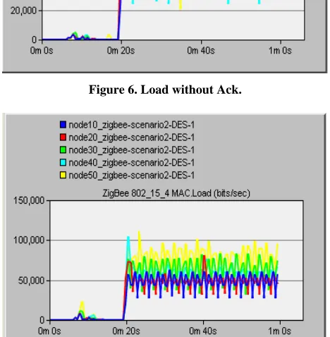
Figures6 and 7 show the load variations of 10, 20, 30, 40, and 50 nodes with and without ACK.

8. Conclusion

When the nodes are static and if each of the nodes is able to communicate with its neighbouring node then there

Figure 6. Load without Ack.

will be minimum delay for establishing the routes to the sink node and for association with the sink node. But if the sink is moving then there can be association problems for the normal sensor nodes with the sink node. The ma- jor factors that decide the Network performance of Mo- bile coordinators are the node density and the traffic. Two key features required for this case scenarios are the ACK enable and understanding the range capability of ZigBee. Placing the end devices too close to the destina-tion coordinator will result in traffic being sent directly, rather than through the router, preventing observations for the self-healing feature. Also the ACK enable was required for the end devices to recognize that the failure in the router has occurred, no longer receiving and rout-ing traffic, in order to trigger route discovery. Thus the load metric for different number of nodes in Hexagonal configuration is obtained by enabling and disabling ACK. If a trajectory has to be chosen for other reasons, then the trajectory should give a considerable amount of time to each route that is the link route for a segment of the net-work. The load of the network may be affected when the trajectory of the coordinator varies.

REFERENCES

[1] Sinem Coleri Ergen, “ZigBee/IEEE 802.15.4 Summary,” 10 September 2004.

[2] A. A. Somasundara, A. Ramamoorthy and M. B. Srivas- tava, “Mobile Element Scheduling for Efficient Data Col- lection in Wireless Sensor Networks with Dynamic Dead- lines,” 25th IEEE International Real-Time Systems Sym- posium (RTSS), Lisbon, 5-8 December 2004, pp. 296-305. doi:10.1109/REAL.2004.31

[3] M. Shakya, J. Zhang, P. Zhang and M. Lampe, “Design and Optimization of Wireless Sensor Network with Mo- bile Gateway,” 21st International Conference on Advanced Information Networking and Applications Workshops

(AINA’07), Niagara Falls, 21-23 May 2007, pp. 415-420. [4] F. Zhao and L. Guibas, “Wireless Sensor Networks—An

Information Processing Approach,” Morgan Kaufmann Publishers, Waltham, pp. 200-203.

[5] E. Ekici, Y. Gu and D. Bozdag, “Mobility-Based Com- munication in Wireless Sensor Networks,” IEEE Com- munications Magazine, Vol. 44, No. 7, 2006, pp. 56-62. doi:10.1109/MCOM.2006.1668382

[6] J. Luo, J. Panchard, M. Piorkowski, M. Grossglauser and J.-P. Hubaux, “MobiRoute: Routing towards a Mobile Sink for Improving Lifetime in Sensor Networks,” 2nd IEEE/ACM International Conference on Distributed Com- puting in Sensor, San Francisco, 18-20 June 2006. [7] Y. Bi, L. Sun, J. Ma, N. Li, I. A. Khan and C. Chen,

“HUMS: An Autonomous Moving Strategy for Mobile Sinks in Data-Gathering Sensor Networks,” EURASIP Journal on Wireless Communications and Networking, 2007, Article ID: 164574.

[8] Z. Vincze and R. Vida, “Multi-Hop Wireless Sensor Net-works with MobileSink”, ACM Conference on Emerging Network Experiment and Technology (CoNEXT’05), Tou- louse, 24-17 October 2005.

[9] Z. Alliance, “Zigbee Specification v1.0,” June 2008. http://www.zigbee.org

[10] OPNET Modeler Inc., November 2008.

http://www.opnet.com/solutions/network_rd/modeler.html