ISSN Print: 1945-3116
On Utilizing Model Transformation for the
Performance Analysis of Queueing Networks
Issam Al-Azzoni
College of Engineering, Al Ain University of Science and Technology, Al Ain, United Arab Emirates
Abstract
In this paper, we present an approach for model transformation from Queueing Network Models (QNMs) into Queueing Petri Nets (QPNs). The performance of QPNs can be analyzed using a powerful simulation engine, SimQPN, designed to exploit the knowledge and behavior of QPNs to im-prove the efficiency of simulation. When QNMs are transformed into QPNs, their performance can be analyzed efficiently using SimQPN. To validate our approach, we apply it to analyze the performance of several queueing network models including a model of a database system. The evaluation results show that the performance analysis of the transformed QNMs has high accuracy and low overhead. In this context, model transformation enables the per-formance analysis of queueing networks using different ways that can be more efficient.
Keywords
Model Transformation, Queueing Networks, Queueing Petri Nets, ATL
1. Introduction
Models have become the de facto standard approach to deal with complexity present in today’s software systems. Model-Driven Engineering (MDE) ap-proaches consider models not just as documentation artifacts, but as central ar-tifacts in the software engineering process [1]. Model transformation is a fun-damental part of MDE. In MDE, a model can be automatically transformed into another model that can be at a different level of abstraction or in a different formalism altogether. In doing so, the generated models can be analyzed in pos-sibly more efficient ways than the original source models. There exist several model transformation languages. In particular, the ATLAS Transformation Language (ATL) [2] is a well-known model transformation language with an How to cite this paper: Al-Azzoni, I.
(2018) On Utilizing Model Transformation for the Performance Analysis of Queueing Networks. Journal of Software Engineering and Applications, 11, 435-457.
https://doi.org/10.4236/jsea.2018.119026
Received: August 16, 2018 Accepted: September 25, 2018 Published: September 28, 2018
Copyright © 2018 by author and Scientific Research Publishing Inc. This work is licensed under the Creative Commons Attribution International License (CC BY 4.0).
http://creativecommons.org/licenses/by/4.0/ Open Access
Integrated Development Environment (IDE) developed on top of the Eclipse platform. The ATL language and toolkit are parts of the Eclipse Modeling Pro-ject (EMP) [3] set of tools and languages which provide MDE capabilities to the Eclipse community.
Queueing network models (QNMs) provide powerful notation for modeling and analyzing the performance of many different kinds of systems [4]. QNMs help in predicting system performance during the design phase. This is useful to detect potential problems before the resources are actually committed. In addi-tion, these performance models help manage design tradeoffs and alternatives. QNMs can be analyzed using analytical techniques or simulation. The analytical techniques allow for quick performance analysis, however these can only be ap-plied on specific kinds of QNMs under several assumptions and conditions. Many QNMs can only be analyzed using simulation. The main drawback of simulation is the incurred computational cost.
An approach to reduce the simulation cost is to transform QNMs into Queueing Petri Nets (QPNs) [5] [6] that have equivalent performance charac-teristics. QPNs provide a powerful general-purpose modeling formalism that can be exploited for modeling systems and analyzing their performance. One tool for analyzing QPNs is QPME [7] which includes a simulation engine (SimQPN [8]) especially optimized to simulate QPNs. SimQPN has been designed to exploit the knowledge of the structure and behavior of QPNs to improve the efficiency of simulation. In [9], the authors conclude that SimQPN executes faster than several other solvers and that it provides a good balance between prediction ac-curacy and overhead. The main challenge of this approach is that QNMs and QPNs are two different formalisms with different notations and constructs. In order to overcome this challenge, developing an automatic transformation from QNMs into QPNs is desired.
This work attempts to fill this gap by presenting an approach for model transformation from QNMs into QPNs. This paper is the journal extension to [10]. In [10], we presented metamodels for QNMs and QPNs using the Ecore meta modeling language [11] and the transformation rules from QNM into QPN models using ATL. In this paper, we generalize the work so that the presented model transformation can be implemented using languages other than ATL. We also include important details, definitions and discussions, validate the model transformation approach using new case studies including a QNM of a database application, and include an overview of the related literature.
The organization of the paper is as follows. First, we provide the necessary background in Section 2. The background covers model transformation, QNMs, and QPNs. In addition, it includes the Ecore metamodels for QNMs and QPNs. Second, we present in Section 3 the rules for transforming QNs into QPNs. Sec-tion 4 discusses two case studies that validate our model transformaSec-tion ap-proach. The related literature is discussed in Section 5. The conclusion and fu-ture work are discussed in Section 6.
2. Background and Definitions
2.1. Model Transformation
Models play a central role in MDE. A model is a reduced presentation of a sys-tem (or more generally any handled isys-tem) that helps to analyze certain proper-ties of the system without the need to consider its full details. Models help de-signers and architects to deal with complexity present in systems.
A model needs to conform to a metamodel. This means that the model needs to satisfy the rules defined in the metamodel and it must respect its semantics. For example, a Petri net model must respect the semantics defined by a Petri net metamodel. In this regard, a metamodel can be considered as a model of models [1]. Since a metamodel is a model itself, it must conform to another meta- metamodel, and so on. In order to avoid having several layers of metamodel re-lationships hierarchy, a meta modeling language is used to specify metamodels. This meta modeling language describes itself in its own language. Thus, a meta-metamodel conforms to itself. Ecore is a meta modeling language used to specify metamodels [11]. The metamodels in the Eclipse Modeling Framework (EMF) [13] are specified in Ecore thus they conform to Ecore which conforms to itself. Going back to the Petri net model example, a Petri net model conforms to a Petri net metamodel which conforms to Ecore which conforms to itself. An-other meta modeling language is the Meta Object Facility (MOF) [14]. MOF is the core meta modeling language in the Model Driven Architecture (MDA) proposed by the OMG [15].
In MDE, models are the main development artifacts. Models can be trans-formed into other models allowing for several types of analysis at different levels of abstraction. Model-to-model transformation is an important operation in MDE. In model-to-model transformation, a source model that conforms to a source metamodel is transformed into a target model that conforms to a target metamodel. A model-to-model transformation language is used to specify the transformation rules. ATL [2] is a well-known model-to-model transformation language that can be used to transform models specified in metamodels con-forming to Ecore or MOF. ATL language and toolkit are parts of the Eclipse Modeling Project set of tools and languages. Analogously, QVT (Query/View/ Transformations) [12] is a set of languages for model query and transformations defined by the OMG. QVT operates on models conforming to MOF.
As a transformation language, ATL is used to specify the way to produce a number of target models from a set of source models. The model transformation in ATL is specified using transformation rules. A transformation rule specifies one or more target model elements to be created for each matched element in the source model. There are three kinds of transformation rules in ATL: matched, lazy, and called rules. Matched and lazy rules allow to specify trans-formation mainly in a declarative fashion while on the other hand the called rules support an imperative style to specify the transformation. Lazy rules are like matched rules, but are only applied when called by other rules. Called rules
have to be explicitly invoked by other rules and can accept parameters. A called rule has to be called from an imperative code section, either from a matched rule or another called rule. It is preferred to use a declarative style when defining the transformation rules [16]. All of the transformation rules presented in this paper are implemented in ATL using matched rules [10].
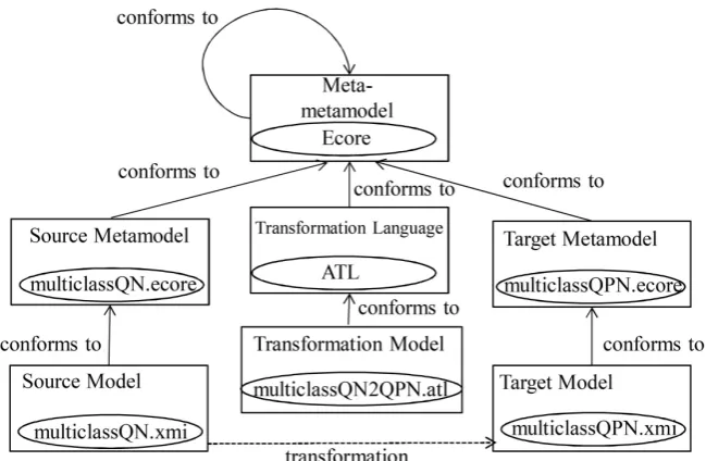
In the context of MDE, the model transformation itself can be considered as a model. It conforms to a transformation metamodel which conforms to another meta-metamodel. ATL is the model transformation language used in [10]. It represents the metamodel. Thus, the ATL module developed in [10] conforms to ATL. ATL itself conforms to Ecore which represents the meta-metamodel. The model transformation process presented in this paper is depicted in Figure 1.
2.2. Queueing Network Models
Queueing network models provide powerful notations for modeling and ana-lyzing the performance of many different kinds of systems [4]. A designer of a software system, for instance, can develop a queueing network model that cap-tures performance-relevant details of the system and then use it to analyze its performance. The model is useful for the designer to verify whether or not per-formance-related requirements are met. In addition, the model can help the de-signer in making design decisions that improve the system performance and to manage design tradeoffs that are typically faced in the design of software sys-tems.
A queueing network is made up of servers. Each server is associated with a queue. Jobs that arrive to a busy server (already executing another job) are queued in the server’s queue. There can be several classes (types) of jobs. Each job class represents a workload in the queueing network. There are two main types of workloads: open and closed. For an open workload, the jobs arrive from outside the network. For a closed workload, the number of jobs inside the net-work is constant and there is no job arriving from outside the netnet-work. The open workload intensity is characterized by the job arrival rates to the servers. On the other hand, the closed workload intensity is characterized by the number of jobs circulating in the network.
A server uses a fixed scheduling policy to choose the next job to serve. First-Come-First-Served (FCFS) and Last-Come-First-Served (LCFS) are exam-ple scheduling policies. When a server serves a job of a given class, the service time refers to the time it takes the job to run on this server. The service time dis-tribution depends on the server and the job class. The Exponential disdis-tribution is a common service time distribution. The distribution parameters are those pa-rameters that are needed to characterize the distribution. For example, the Ex-ponential distribution requires a single parameter: the rate
µ
. For the Expo-nential distribution, the mean is 1µ. For a server, the service time distribu-tions and their parameters need to be specified for all job classes that can be served by the server.Figure 1. The model transformation process (ATL is used here as a sample model trans-formation language).
For an open class workload, jobs arrive from outside the network. Jobs of a given class can arrive to one or more servers. The arrival time distributions and their parameters need to be specified for each job class at each server. The Pois-son distribution is a common arrival time distribution and it requires a single parameter
λ
. For a closed class workload, the workload intensity is character-ized by the number of jobs circulating in the network. Thus, the number of jobs needs to be specified. In order to model interactive systems, a think device is used for closed class workloads. A think device can be thought of as an infinite server farm that can serve any incoming job immediately. The think device re-quires a think time distribution and its parameters.When a job is served by a server, it can be routed to another server or outside the network. We consider networks of queues with probabilistic routing. For a job of class c, Pi j,c denotes the probability that job at server i of class c next moves to server j. Pi out,c denotes the probability that job at server i of class c is routed outside the network after it is served by the server i. The routing prob-abilities need to be completely specified for all workloads in a given queueing network.
There are several performance metrics that can be computed for a given queueing network model. These include the average job response time T, the av-erage number of jobs in the system N, and the utilization and throughput for a given server. The job response time is the time difference between the time when the job leaves the system and the time when the job arrived to the system. The number of jobs in the system includes those jobs in the queues plus the ones be-ing served. For multi-classed networks, T and N can be computed at a class level basis. The utilization of a server is the fraction of time the sever is busy. The throughput of a server is the rate of job completions at the server. In this paper,
we use several performance metrics to validate the model-to-model transforma-tion.
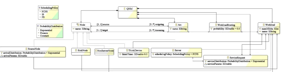
Figure 2 shows the Ecore metamodel for queueing networks. A queueing network model is composed of one or more Nodes, zero or more Arcs, one or more Workloads, zero or more WorkloadRoutings, and zero or more Ser-viceRequests. The Arc class connects nodes. For any given arc, there is one source node and one target node. Node is an abstract class and there are five types of nodes: SourceNode, SinkNode, NonServerNode, ThinkDevice and Server. SourceNodes and SinkNodes are used for open workloads to represent the entry and exit points. ThinkDevice node is used to represent the think device. A NonServerNode is optionally used in batch processing closed workloads in which there is no think device. In such workloads, we can use a NonServerNode to re-route a job after it finishes service to a server so that the job starts a new service cycle with a think time of zero. A Server node provides a processing ser-vice. A Server has a scheduling policy represented by the attribute scheduling Policy whose type is the enumerated type SchedulingPolicy. In Figure 2, we in-clude representative scheduling policies that are used in the case studies pre-sented in the paper. Note that the attributes arrivalDistribution and arrivalPar-ams are used in SourceNode class to characterize the arrival time process in open workloads.
A Workload has an optional name and a numOfJobs attribute used in closed workloads to represent the number of jobs. A Server is associated with zero to many Workloads. For the other types of nodes, a node is associated with one Workload. This is because a server may serve jobs of different workloads. A Ser-vice Request associates Workloads with Servers. SerSer-vice Requests represent the service times. Since the service time of a job depends on its class (workload) and the server, the relations from ServiceRequest to Server and ServiceRequest to Workload are one to one in both cases. The ServiceRequest class has two attrib-utes used to characterize the service time: serviceDistribution and serviceParams. The value of the first attribute sets the service time distribution. An enumerated type, Probability Distribution, is used to enumerate the supported probability distributions. We only include the three distributions used in the case studies, however the tool QPME supports several others as well. The distribution pa-rameters are represented by the sequence service Params. The job routing prob-abilities are represented using WorkloadRoutings. Each Workload Routing is a associated with one Arc and one Workload and it has a probability property. For example, to represent the routing probability Pi j,c , the modeler creates a Work-load Routing whose probability is set to Pi j,c. The Workload Routing is associ-ated with the Arc from Server i to Server j and with the Workload representing job class c.
The metamodel shown in Figure 2 can be used to define a wide variety of queueing network models including networks which have no product-form so-lutions. However, the metamodel cannot capture networks having one or more of the following features:
Figure 2. The Ecore metamodel for queueing Networks.
1) Jobs can change classes after being served. 2) Some servers have load-dependent service times. 3) Some servers have finite queue capacities. 4) Job routing is not probabilistic.
Our metamodel is similar to the ePMIF metamodel [17]. However, there are three main differences. First, we do not specialize the Workload class into its subclasses: Open Workload and Closed Workload. The distinction is not neces-sary when transforming the queueing network into a queueing Petri net. Second, we use Workload Routing class to represent the job routing probabilities. In ePMIF, these are represented by attributes. The use of references rather than at-tributes to refer to objects is a better practice [16]. Third, ePMIF specializes Ser-vice Request into three types: Work Unit SerSer-vice Request, Time SerSer-vice Request, and Demand Service Request. Service Request class is used to define job service times. Our metamodel assumes Time Service Request service time definition only. Work Unit Service Requests can be alternatively defined by using a se-quence of Time Service Requests. In Demand Service Request, the service time is specified in terms of the service demand and the number of visits. Our meta-model does not support Demand Service Requests since these cannot be incor-porated easily into queueing Petri nets.
2.3. Queueing Petri Nets
Queueing Petri nets extend Colored Generalized Stochastic Petri Nets (CGSPNs) by allowing queues to be integrated into places of CGSPNs. In QPNs, there are two types of places: ordinary places and queueing places. The ordinary places are defined the same way as in CGSPNs. Queueing places, on the other hand, add queueing and timing aspects to the places of CGSPNs. A queueing place consists of two components: a queue and a depository. When an input transition of a queueing place fires, tokens are inserted into the queue of the queueing place according to the queue’s scheduling policy. After completion of its service, a to-ken is moved to the depository where it becomes available for the output transi-tions of the place. The queue has an associated service station for which service time distribution needs to be defined. QPNs strengthen the power of CGSPNs modeling by the direct inclusion of queueing aspects into their models. The reader is referred to [5] [6] for more comprehensive overview of QPNs.
Formally, a QPN is an 8-tuple QPN=
(
P T C I I M Q W, , , , ,− + 0, ,)
[6] where: 1) P={
p p1, , ,2 pn}
is a finite and non-empty set of places.2) T=
{
t t1 2, , , tm}
is a finite and non-empty set of transitions.3) C is a color function that maps each place to a finite and non-empty set of colors and maps each transition to a finite and non-empty set of modes. 4) I− and I+ are the backward and forward incidence functions defined on
P T× , such that I p t I p t−
( ) ( )
, , + , ∈C t( )
→C p( )
MS , ∀
( )
p t, ∈ ×P T.( )
MSC p denotes the set of all finite multisets of C p
( )
. 5) M0 is a function that maps each place to its initial marking( )
( )
(
M p C p0 ∈ MS)
.6) Q=
(
Q q1, , ,(
1 qP)
)
where Q1⊆P is the set of queueing places, and qidenotes the description of a queue taking all colors of C p
( )
i intoconsid-eration, if pi is a queueing place or equals “null”, if pi is an ordinary
place.
7) W =
(
W W w 1, ,2(
1, , wT)
)
where W1⊆T is the set of timed transitions, 2W ⊆T is the set of immediate transitions, W W1 2=φ and W W T1 2= , and wi∈C t
( )
i →+ is a function such that ∀ ∈c C t w c( ) ( )
i : i is [image:8.595.286.464.593.701.2]interpreted as a rate of a negative Exponential distribution specifying the fir-ing delay due to color (mode) c if t Wi∈ 1 or a firing weight specifying the relative firing frequency due to color (mode) c if t Wi∈ 2.
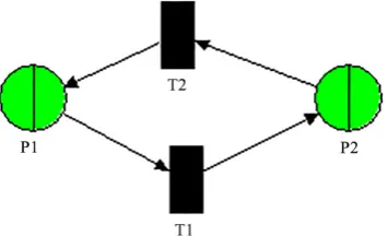
Figure 3 shows an example QPN. It models a queueing network that has a single server and a think device. There are two closed workloads: the first one has a single job and the second one has two jobs. The QPN has two queueing places: P1 and P2. There are two immediate transitions connecting the queueing places: T1 and T2. Place P1 models the think device. The scheduling policy of its queue is set to Infinite Server. The place P2 models a CPU server whose queue’s scheduling policy is set to Processor-Sharing. There are two colors associated with both places: C P
( )
1 =C P( ) {
2 = c c1, 2}
. In the initial marking, the deposi-tory of place P1 contains one token of color c1 and two tokens of color c2. For the colors on both queueing places, we can set the service time distributions and their parameters to match their corresponding queueing network’s ones. We as-sociate two modes with each transition. Each mode connects a single token from an input place to a single token (of the same color) on the output place. Modes are used to define the incidence function of transitions.Figure 3. An example QPN model.
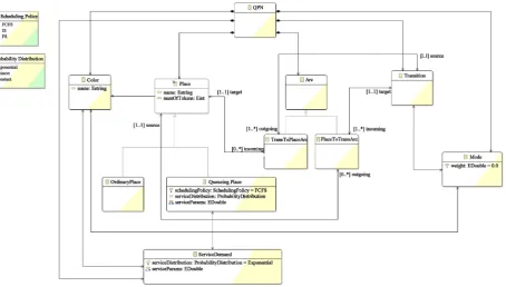
Figure 4 shows the Ecore metamodel for QPNs. A QPN model is composed of one or more Places, zero or more Transitions, zero or more Arcs, zero or more Modes, zero or more Service Demands, and one or more Colors. The Arc class connects places to transitions and vice-versa: TransToPlaceArc connects a Tran-sition to a Place and PlaceToTransArc connects a Place to a TranTran-sition. There are two types of places: Queueing Places and Ordinary Places. A Queueing Place has the necessary attributes to define the scheduling policy of its queue. A Place is associated with one or more Colors. A Place has a name and numOfTokens attribute which sets the initial marking. When a place has more than one color, it is necessary to define the token service time distribution and the distribution parameters for each color. This is achieved by using a Service Demand object that associates one Queueing Place with a single Color. If a queueing place has a single color, it suffices to define the token service time distribution and its pa-rameters by using the attributes of the Queueing Place, service Distribution and service Params, without the need to use any Service Demand object. A Transi-tion is associated with one or more Modes. The Mode class has a single attribute defining the firing weight of the mode.
We use QPME (Queueing Petri net Modeling Environment) [7] tool to create the QPNs and to analyze their models. QPME is an open-source tool for the stochastic modeling and analysis of QPNs. QPME has a discrete-event simula-tion engine specialized for QPNs. It exploits the knowledge of the structure and behavior of QPNs to improve the efficiency of simulation. Using simulation in QPME, many performance metrics can be computed including metrics defined on the token response times, queue utilization, and token population and occu-pancy.
Figure 4. The Ecore metamodel for queueing Petri nets.
3. Model Transformation of QNMs into QPNs
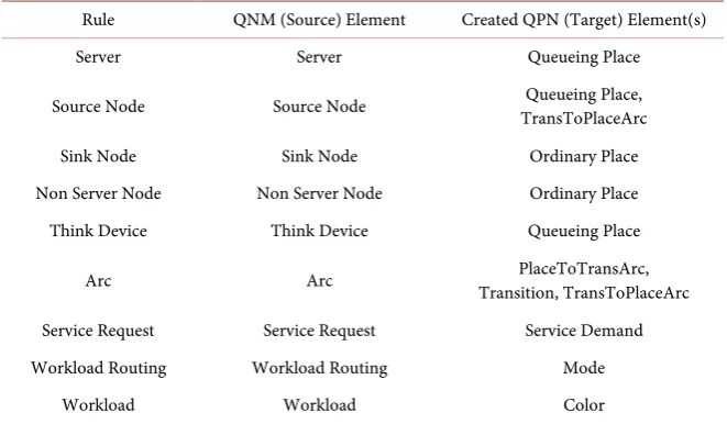
Table 1 gives an overview of the transformation rules (the ATL implementation can be found in [10]). There are ten rules:
1) Rule Main generates a QPN element from the input QNM element. Its set of places, transitions, modes, colors, and service demands respectively corre-spond to the elements generated for the nodes, the arcs, the Workload Rout-ings, the Workloads, and the Service Requests of the input QNM. Its set of arcs correspond to the “qpn_ia”, “qpn_oa” and “qpn_oas” elements gener-ated for the input Arc elements.
2) Rule Server generates an Queueing Place element from an input Server ele-ment. The name of the Queueing Place element is the same as the name of the Server element. The scheduling policy of the Queueing Place is set to the same scheduling policy as that of the Server. The colors of the Queueing Place correspond to the color elements that are generated for the workloads of the Server. The incoming arcs of the Queueing Place correspond to the TransToPlaceArcs that are generated for the incoming arcs of the Server. The outgoing arcs of the Queueing Place correspond to the PlaceToTransArcs that are generated for the outgoing arcs of the Server.
3) Rule Source Node generates a Queueing Place element and a TransTo-PlaceArc element from an input Source Node element. A Source Node ele-ment is assumed to have one outgoing arc. In a QPN, the arrival of jobs in an open workload can be modeled using a queueing place having the scheduling policy of Infinite Server (IS) and the number of tokens being set to one. After the token is served, the token is returned to the place by using a TransTo-PlaceArc from the transition that is generated for the arc connecting the SourceNode and its outgoing arc to the queueing place. The name of the QueueingPlace element is the same as the name of the SourceNode element. The scheduling policy of the Queueing Place is set to Infinite Server (IS). The serviceDistribution and serviceParams properties of the QueueingPlace ele-ment correspond to the same properties of the SourceNode eleele-ment. The color of the QueueingPlace corresponds to the color element that is gener-ated for the workload of the SourceNode. The incoming arc of the Queueing Place corresponds to the TransToPlaceArc that is generated from the Sour-ceNode. The outgoing arc of the QueueingPlace corresponds to the PlaceTo-TransArc that is generated for the outgoing arc of the SourceNode. The source of the generated TransToPlaceArc corresponds to the transition that is generated for the arc connecting the SourceNode and its outgoing arc. The target of the generated TransToPlaceArc corresponds to the generated QueueingPlace element.
4) Rule SinkNode generates an OrdinaryPlace element from an input SinkNode element. The name of the OrdinaryPlace element is the same as the name of the SinkNode element. The color of the SinkNode corresponds to the color element that is generated for the workload of the SinkNode. The incoming
Table 1. The transformation rules.
Rule QNM (Source) Element Created QPN (Target) Element(s)
Server Server Queueing Place
Source Node Source Node TransToPlaceArc Queueing Place,
Sink Node Sink Node Ordinary Place Non Server Node Non Server Node Ordinary Place Think Device Think Device Queueing Place
Arc Arc Transition, TransToPlaceArc PlaceToTransArc,
Service Request Service Request Service Demand Workload Routing Workload Routing Mode
Workload Workload Color
arcs of the Ordinary Place correspond to the TransToPlaceArcs that are gen-erated for the incoming arcs of the SinkNode. The outgoing arcs of the Or-dinaryPlace correspond to the PlaceToTransArcs that are generated for the outgoing arcs of the SinkNode.
5) Rule NonServerNode generates an OrdinaryPlace element from an input NonServerNode element. The name of the OrdinaryPlace element is the same as the name of the NonServerNode element. A NonServerNode is used in a batch processing closed workload in which there is no think device. Hence, numOfTokens property of the OrdinaryPlace is set the numOfJobs property of the workload linked to the NonServerNode. The color of the Or-dinaryPlace corresponds to the color element that is generated for the work-load of the NonServerNode. The incoming arcs of the OrdinaryPlace corre-spond to the TransToPlaceArcs that are generated for the incoming arcs of the NonServerNode. The outgoing arcs of the OrdinaryPlace correspond to the PlaceToTransArcs that are generated for the outgoing arcs of the None-ServerNode.
6) Rule Think Device generates a Queueing Place element from an input ThinkDevice element. The name of the QueueingPlace element is the same as the name of the ThinkDevice element. The scheduling policy of the Queue-ingPlace is set to Infinite Server (IS). For the generated QueueQueue-ingPlace, the service time distribution is assumed to be Exponential and the list of distri-bution parameters contains a single parameter: the average think time. For a closed workload, the number of jobs inside the network is constant. It is equal to the numOfJobs property of the workload linked to the ThinkDevice. The color of the QueueingPlace corresponds to the color element that is gen-erated for the workload of the ThinkDevice. The incoming arcs of the QueueingPlace correspond to the TransToPlaceArcs that are generated for the incoming arcs of the ThinkDevice. The outgoing arcs of the
Place correspond to the PlaceToTransArcs that are generated for the outgo-ing arcs of the ThinkDevice.
7) Rule Arc generates three elements from an input Arc element: Transition, PlaceToTransArc, and TransToPlaceArc. The incoming arc of the generated transition corresponds to the PlacetoTransArc element that is generated for the Arc element. The outgoing arc of the generated transition corresponds to the TransToPlaceArc element that is generated for the Arc element. The source of the PlaceToTransArc corresponds to the source element that is generated for the Arc element. The target of the TransToPlaceArc corre-sponds to the target element that is generated for the Arc element. The gen-erated Transition is set to be the target for the gengen-erated PlaceToTransArc as well as the source for the generated TransToPlaceArc.
8) Rule ServiceRequest generates a ServiceDemand element from an input Ser-viceRequest element. The serviceDistribution and serviceParams properties of the ServiceDemand element correspond to the same properties of the Ser-viceRequest element. Its queueingPlace and color correspond to the queueing place and color elements that are generated for the server and workload of the ServiceRequest element, respectively.
9) Rule Workload Routing generates a Mode element from an input Work-loadRouting element. The mode’s firing weight corresponds to the probabil-ity property of the WorkloadRouting element. Its transition and color corre-spond to the transition and color elements that are generated for the arc and workload of the WorkloadRouting element, respectively.
10) Rule Workload generates a Color element from an input Workload element with the same name.
4. Evaluation
In this section, we validate our model transformation using two cases studies. The first case study uses a QN model of a computer system having a CPU and an I/O device. The second case study uses a QN model developed in the context of the performance evaluation of a data base design. A third case study is presented in [10].
4.1. Case Study 1: CPU-Bound and I/O-Bound Jobs Example
In this case study, we discuss a queueing network model used in [4]. It models a computer system having a CPU device and an I/O device. The queueing network model is shown in Figure 5. There are two different types of jobs: CPU-bound jobs and I/O-bound jobs. The workload consisting of CPU-bound jobs is labeled with superscript C. Similarly, the workload consisting of I/O-bound jobs is la-beled with superscript I. Both are open workloads. The CPU device has an Ex-ponential service rate of 2 jobs per second and the I/O device has an ExEx-ponential service rate of 1 job per second. The service rates are independent from the type of jobs. Jobs of a given type arrive from outside the network according to aPoisson process. The rates are shown in the figure. Two performance metrics are to be computed: the average response time of CPU-bound jobs and the average number of CPU-bound jobs at the CPU.
In the QN model corresponding to Figure 5, there are 6 nodes: two servers, two source nodes, and two sink nodes. There are two open workloads and each workload has its own source and sink nodes. There are 11 arcs connecting the nodes. Each arc is associated with a single WorkloadRouting element whose probability value is set to the corresponding routing probability in Figure 5. Thus, there are 11 WorkloadRouting elements. There are four ServiceRequest elements that are used to define the service rates: each device serves both work-loads.
The resulting QPN model is shown in Figure 6. It consists of six places: four queueing places and two ordinary places. For each server or source node in the source QN model, there is one corresponding queueing place in the target QPN model. For each sink node in the source QN model, there is one corresponding ordinary place in the target QPN model. There are two colors: one color corre-sponding to each workload in the source QN model. There are 11 transitions: one transition for each arc in the source QN model. Each transition is associated with a single mode whose firing weight is equal to the corresponding arc’s Workload Routing probability. There are four Service Demands: one Ser-viceDemand for each ServiceRequest in the source QN model. There are 24 arcs in the target QPN model: 22 arcs are generated by rule Arc while two arcs are generated by rule SourceNode.
Table 2 compares several performance metrics computed analytically using queueing theory with the results of QPME simulation. The details of how the analytic results are determined can be found in Chapter 18 of [4]. The table in-cludes server utilization, the average number of jobs at each server, and the av-erage job response time at each server. In addition, the table includes the two performance metrics defined in Section 2.2. The table demonstrates the high ac-curacy of QPME simulation. All performance metrics were directly returned by QPME except the average response time of the CPU-bound jobs. For this one, one needs to calculate the expected number of times a CPU-bound job visits the CPU and the I/O-Device. Let E V 1C and E V 2C be the expected number of times a CPU-bound job visits the CPU and the I/O-Device, respectively. Then, we obtain E V 1C and E V 2C by solving the following system of equations:
1C 1 0.65 1C 1.0 1C
E V = + E V + E V
2C 0.05 1C E V = E V
The details can be found in Chapter 18 of [4]. Solving the system of equations, we obtain E V 1C = 3.333 and E V 2C = 0.167. Then, we calculate the average response time of the CPU-bound jobs as follows: E V 1C × (Average Job’s Re-sponse Time − CPU) + E V 3C × (Average Job’s Response Time − I/O-Device)
3.333 0.789 0.167 2.928 3.119
= × + × = .
Figure 5. Queueing network example: CPU-bound and I/O-bound jobs (based on Figure 18.6 in [4]).
Figure 6. The QPN corresponding to the queueing network of Figure 5.
[image:14.595.172.534.308.704.2]Table 2. A comparison between the analytic and QPME simulation results for the net-work of Figure 5.
Performance Metric Analytic Result QPME Simulation Result
Utilization—CPU 0.366 0.366
Utilization—I/O-Device 0.658 0.659 Average Number of Jobs—CPU 0.578 0.577
Average Number of
Jobs—I/O-Device 1.927 1.927
Average Job’s Response
Time—CPU 0.790 0.789
Average Job’s Response
Time—I/O-Device 2.927 2.928
Average Response Time of
CPU-bound Jobs 3.117 3.119
Average Number of CPU-bound
jobs at the CPU 0.526 0.526
4.2. Case Study 2: Database Design
In this case study, we validate our model transformation approach using the queueing network model developed in the context of the performance evaluation of a database design in [18]. The Transaction Processing Performance Council (TPC) TPC-C benchmark is used as the example of the database system design [19]. TPC-C is an on-line transaction processing (OLTP) benchmark designed to be representative of actual production applications and environments.
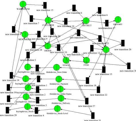
The TPC-C benchmark is a design specification of an order-entry system. In the QNM developed in [18], each table in the database design is modeled as a server and each transaction type is modeled as a separate customer class (work-load). In TPC-C benchmark specification, there are nine tables (WAREHOUSE, DISTRICT, CUSTOMER, HISTORY, ORDER, NEW-ORDER, ORDER-LINE, STOCK, ITEM) and five transaction types (New-Order, Payment, Order-Status, Delivery, Stock-Level). Figure 5 shows the multi-class QNM for the TPC-C benchmark. The queueing discipline of all servers is assumed to be FCFS and the queue lengths are assumed infinite [18].
As Figure 7 shows, the five workloads are all closed. Each workload has a mean keying time and a think time. These are shown in Table 3. Since the benchmark is trying to emulate a real user environment, when a user (client) re-ceives the result of transaction i, the client will spend some time processing that data (think time of transaction i) before choosing a new transaction and keying in its parameters (keying time for transaction i + 1). The TPC-C benchmark specifies that the transaction think times follow an Exponential distribution. The keying times are deterministically distributed. Table 3 also includes the specified percentage of the total number of transactions by the TPC-C benchmark for each workload.
Table 3. Summary of the TPC-benchmark transactions (based on [18]).
Transaction The specified percentage of the total number of transactions
Mean think time
distribution (seconds) Keying time (seconds)
New-Order 45 12 18
Payment 43 12 3
Order-Status 4 10 2
Delivery 4 5 2
Stock-Level 4 5 2
Figure 7. The QNM for the TPC-C benchmark (the figure is reproduced from [18]).
Table 4 shows the mean service demands for the TPC-C benchmark specified as numbers of database I/O pages. In the simulation experiments of [18], the ac-cess time for a single database I/O page is assumed 0.00002 seconds (refer to Ta-ble 6 in [18]). Using this information, the mean service demands can be com-puted for all workloads on each server in millisecond time unit. The service de-mands are assumed exponentially distributed as in [18].
In the source QNM, there are 19 nodes: 14 servers corresponding to the tables and the keying devices and five think devices. There are five closed workloads. There are 32 arcs connecting the nodes. Each arc is associated with a single WorkloadRouting element having probability that is equal to one. Thus, there are 32 WorkloadRouting elements. Each WorkloadRouting element is associated with one workload. There are 50 ServiceRequest elements that are used to define the service rates: all of the entries in Table 4 in addition to the five service rates which characterize the keying times.
Table 4. The service demands for the TPC-C benchmark (based on [18]).
Workload I II III IV V VI VII VIII IX New-Order 1.2 2.2 1.2 0 2.2 2.2 7.3 7.3 4
Payment 2.2 2.2 12.76 2 0 0 0 0 0 Order-Status 0 0 15.51 0 3.45 0 4.63 0 0 Delivery 0 0 7.3 0 13.2 19.7 15.4 0 0 Stock-Level 0 1.2 0 0 0 0 10.63 200.76 0 I = WAREHOUSE, II = DISTRICT, III = CUSTOMER, IV = HISTORY, V = ORDER, VI = NEW-ORDER, VII = ORDER-LINE, VIII = STOCK, IX = ITEM.
The resulting QPN model is shown in Figure 8. It consists of 19 queueing places. For each server or think device in the source QNM, there is a corre-sponding queueing place in the target QPN model. There are five colors: one color corresponding to each workload in the source QNM. There are 32 transi-tions: one transition for each arc in the source QNM. Each transition is associ-ated with a single mode whose firing weight is equal to the corresponding arc’s WorkloadRouting probability. There are 50 ServiceDemands: one ServiceDe-mand for each ServiceRequest in the source QNM. There are 64 arcs in the tar-get QPN; all of them are generated by rule Arc.
For the case study, we are interested in computing the following performance metrics: the average transaction response time for each transaction type. We use SimQPN which is the simulation engine for QPME. First, we create a QPN that corresponds to the target QPN model generated by the ATL transformation process. Then, we run the simulation engine using the default parameters. For instance, the verbosity level is set to 3 by default. This verbosity level sets the data collection level mode to collect the following token residence time data: maximum, minimum, mean, standard deviation, steady state mean, and confi-dence interval of steady state mean. Following a simulation run, we use the QPME Advance Query Editor to query the performance metrics of interest. The wall-clock simulation time is displayed in the main console at the end of the simulation run.
In order to validate the results and to compare against other tools, we use the Java Modeling Tools (JMT) [20] to create and analyze the QNM. We use the JSIMgraph application in the JMT which allows to create a QNM graphically and uses simulation to analyze the performance of the QNM. The default simu-lation parameters are used including a specified confidence interval of 99% for each performance metric to be computed. The simulation times are obtained from the simulation log files.
Table 5 and Table 6 show the simulation results obtained using QPME and JMT under two different loads. The first table shows results assuming 1000 cli-ents while the second table shows results assuming 2000 clicli-ents. The average re-sponse time for each transaction type is shown. In addition, we show the simula-tion time for each tool. The simulasimula-tion runs are carried out on a Dell desktop computer equipped with a 3.00 GHz dual-core processor and 2 GB RAM.
Figure 8. The QPN corresponding to the QNM for the case study.
Table 5. A comparison between the simulation results of QPME and JMT—1000 clients.
QPME JMT
Transaction Type
Average Response Time (milliseconds)
Simulation Time (seconds)
Average Response Time (milliseconds)
Simulation Time (seconds)
New-Order 0.697
9.2
0.651
53.4
Payment 0.386 0.387
Order-Status 0.477 0.477
Delivery 1.117 1.115
Stock-Level 4.388 4.372
[image:18.595.211.539.551.727.2]Table 6. A comparison between the simulation results of QPME and JMT—1500 clients.
QPME JMT
Transaction Type
Average Response Time (milliseconds)
Simulation Time (seconds)
Average Response Time (milliseconds)
Simulation Time (seconds)
New-Order 0.769
12.8
0.699
60.2
Payment 0.388 0.386
Order-Status 0.479 0.481
Delivery 1.121 1.117
Stock-Level 4.442 4.359
The results presented in Table 5 and Table 6 demonstrate good accuracy of QPME simulation. In addition, the results demonstrate that the simulation en-gine in QPME is significantly faster than JMT. We have also validated the results by comparing with the results reported in Figure 4 of [18]. This confirms the finding of Brosig et al.[9] that SimQPN performs fast simulation and provides a good balance between prediction overhead and accuracy.
5. Literature Review
Meier et al. present an approach to transform a Palladio Component Model (PCM) into a QPN model [21]. The transformation is implemented using QVT Operational component [12] and Java. The authors demonstrate that trans-forming the PCM into a QPN model and using the QPN simulator for perform-ance analysis result in good accuracy with solution overhead up to 20 times lower compared to PCM’s main solver. This demonstrates the benefits of trans-formation into QPNs and using their specialized analysis tools such as QPME. The Palladio Component Model (PCM) [22] is a domain-specific modeling lan-guage for component-based systems. On the other hand, queueing networks provide general modeling notation that can be applied in several domains and be exploited for performance analysis.
An approach for transforming a PCM into a Layered Queueing Network (LQN) is presented in [23]. LQNs extend ordinary QNs by concepts such as lay-ers and software servlay-ers, and they allow the modeling of simultaneous resource possession. LQNs have been developed as domain-specific performance model-ing language with a special focus on software and hardware systems. LQNs can model software and hardware contention, synchronization, and blocking in a uniform way. LQNs also have specialized solvers that are used to analyze per-formance. The authors of [23] implement the transformation from PCMs into LQNs in Java. The analytical LQN solver used in [23] relies on Mean Value Analysis (MVA). It allows quicker performance analysis faster than running the PCM discrete-event simulator in many cases, however it can only compute mean values.
In [17], the authors propose an Ecore metamodel for queueing network mod-els. The metamodel is named ePMIF and is based on the PMIF 2 metamodel [24]. The authors use ePMIF to define a Domain Specific Language (DSL) for the specification and analysis of queueing networks. The authors use ATL to trans-form queueing network models contrans-forming to ePMIF into structural and be-havioral models that are subsequently used in the context of the e-Motions tool [25]. The e-Motions tool transforms these models (using ATL transformations) into the corresponding formal specifications in Real-Time Maude [26]. Maude specifications are executable, and therefore they can be used to run simulations.
The authors of [27] present an approach to transform models of network in-frastructures in modern data centers into queueing Petri net models. The se-lected meta-model for the network infrastructures is the Descartes Network In-frastructure (DNI) meta-model for which the Ecore definition is presented in [28]. The transformation approach was presented informally using a case study, however, it was not implemented on any transformation toolkit. The case study shows that the QPN models can predict the utilization of resources with good accuracy within a short time.
In [29], the authors develop ATL transformation from queueing network models into Generalized Stochastic Petri Nets (GSPNs) [30]. The queueing net-work models conform to the Performance Model Interchange Format (PMIF) metamodel [31]. The authors develop a meta-model for GSPNS that can be used to import models for performance analysis in the PIPE2 (Platform Independent Petri Net Editor 2) tool [32]. PIPE2 is a tool to create and analyze GSPNs. A case study demonstrates high accuracy in the performance prediction of throughput and queue lengths. Our meta-model for QNs supports multiple workloads. In addition, the timed transitions in GSPNs have a negative Exponential distribu-tion firing delay. The queueing places in the QPNs considered in this paper can have an arbitrary service time distribution. Thus, our model transformation ap-proach can be applied to model and analyze a wider variety of QNs.
6. Conclusion and Future Work
In this work, we have presented an approach for transforming QNMs into QPNs. The approach was validated using several case studies in which several per-formance metrics were predicted with high accuracy. Our approach can be ap-plied on QNMs with several workloads (job classes) that can be of different types (open and closed). The QNMs supported by our approach need not be of prod-uct form.
The following points outline the main ideas in our future work. First, it is of interest to expand the queueing network metamodel to support new features such as those mentioned at the end of Section 1. Second, we can supplement the QNM and QPN metamodels with OCL constrains [33] [34] to precisely define their valid models in a way that cannot be captured by the structured rules of Ecore. Thereafter, we can apply techniques such as the one in [35] for model
transformation verification to prove a Hoare-style notion partial correctness, i.e., whether the output model produced by a transformation is valid for any valid input model. In this case, we can also apply other techniques for model trans-formation testing, including white-box [36] and black-box approaches [37].
Conflicts of Interest
The authors declare no conflicts of interest regarding the publication of this pa-per.
References
[1] da Silva, A.R. (2015) Model-Driven Engineering: A Survey Supported by the Uni-fied Conceptual Mode. Computer Languages, Systems & Structures, 43, 139-155.
https://doi.org/10.1016/j.cl.2015.06.001
[2] ATL. http://www.eclipse.org/atl/
[3] Eclipse Modeling Project. https://eclipse.org/modeling/
[4] Harchol-Balter, M. (2013) Performance Modeling and Design of Computer Sys-tems: Queueing Theory in Action. Cambridge University Press, Cambridge. [5] Kounev, S. (2006) Performance Modeling and Evaluation of Distributed
Compo-nent-Based Systems Using Queueing Petri Nets. IEEE Transactions on Software Engineering, 32, 486-502. https://doi.org/10.1109/TSE.2006.69
[6] Kounev, S., Spinner, S. and Meier, P. (2012) Introduction to Queueing Petri Nets: Modeling Formalism, Tool Support and Case Studies. Proceedings of the 3rd ACM/SPEC International Conference on Performance Engineering, Boston, 22-25 April 2012, 9-18. https://doi.org/10.1145/2188286.2188290
[7] QPME. http://qpme.sourceforge.net/
[8] Kounev, S. and Buchmann, A. (2006) SimQPN: A Tool and Methodology for Ana-lyzing Queueing Petri Net Models by Means of Simulation. Performance Evalua-tion, 63, 364-394. https://doi.org/10.1016/j.peva.2005.03.004
[9] Brosig, F., Meier, P., Becker, S., Koziolek, A., Koziolek, H. and Kounev, S. (2015) Quantitative Evaluation of Model-Driven Performance Analysis and Simulation of Component-Based Architectures. IEEE Transactions on Software Engineering, 41, 157-175. https://doi.org/10.1109/TSE.2014.2362755
[10] Al-Azzoni, I. (2017) ATL Transformation of Queueing Networks to Queueing Petri Nets. Proceedings of the 5th International Conference on Model-Driven Engineer-ing and Software Development (MODELSWARD), 261-268.
https://doi.org/10.5220/0006110002610268
[11] Steinberg, D., Budinsky, F., Paternostro, M. and Merks, E. (2008) EMF: Eclipse Modeling Framework. 2nd Edition, Addison-Wesley Professional, Ch. 5.
[12] QVT. http://www.omg.org/spec/QVT/
[13] Eclipse Modeling Framework. https://eclipse.org/modeling/emf/
[14] OMG’s MetaObject Facility. http://www.omg.org/mof/ [15] MDA. http://www.omg.org/mda/
[16] Allilaire, F., Bézivin, J., Jouault, F. and Kurtev, I. (2006) ATL: Eclipse Support for Model Transformation. Proceedings of the Eclipse Technology Exchange Workshop of the European Conference on Object-Oriented Programming, Nantes, 4 July 2006.
[17] Troya, J. and Vallecillo, A. (2014) Specification and Simulation of Queueing Net-work Models Using Domain-Specific Languages. Computer Standards & Interfaces, 36, 863-879.https://doi.org/10.1016/j.csi.2014.01.002
[18] Osman, R., Awan, I. and Woodward, M.E. (2009) Application of Queueing Network Models in the Performance Evaluation of Database Designs. Electronic Notes in Theoretical Computer Science, 232, 101-124.
https://doi.org/10.1016/j.entcs.2009.02.053
[19] Overview of the TPC-C Benchmark: The Order-Entry Benchmark.
http://www.tpc.org/tpcc/detail.asp
[20] Java Modeling Tools. http://jmt.sourceforge.net/
[21] Meier, P., Kounev, S. and Koziolek, H. (2011) Automated Transformation of Com-ponent-Based Software Architecture Models to Queueing Petri Nets. Proceedings of the Symposium on Modelling, Analysis, and Simulation of Computer and Tele-communication Systems, Singapore, 25-27 July 2011, 339-348.
[22] Becker, S., Koziolek, H. and Reussner, R. (2009) The Palladio Component Model for Model-Driven Performance Prediction. Journal of Systems and Software, 82, 3-22. https://doi.org/10.1016/j.jss.2008.03.066
[23] Koziolek, H. and Reussner, R. (2008) A Model Transformation from the Palladio Component Model to Layered Queueing Networks. Proceedings of the SPEC Inter-national Performance Evaluation Workshop, Darmstadt, 27-28 June 2008, 58-78. https://doi.org/10.1007/978-3-540-69814-2_6
[24] Smith, C.U., Lladó, C.M. and Puigjaner, R. (2010) Performance Model Interchange Format (PMIF 2): A Comprehensive Approach to Queueing Network Model Inte-roperability. Performance Evaluation, 67, 548-568.
https://doi.org/10.1016/j.peva.2010.01.006
[25] The e-Motions Tool.
http://atenea.lcc.uma.es/index.php/Main_Page/Resources/E-motions
[26] Clavel, M., Durán, F., Eker, S., Lincoln, P., Mart-Oliet, N., Meseguer, J. and Talcott, C. (2007) All About Maude—A High-Performance Logical Framework: How to Specify, Program and Verify Systems in Rewriting Logic. Springer-Verlag, Berlin. [27] Rygielski, P. and Kounev, S. (2014) Data Center Network Throughput Analysis
Us-ing QueueUs-ing Petri Nets. Proceedings of the Conference on Distributed Computing Systems Workshops, Madrid, 30 June-3 July 2014, 100-105.
https://doi.org/10.1109/ICDCSW.2014.11
[28] Rygielski, P., Zschaler, S. and Kounev, S. (2013) A Meta-Model for Performance Modeling of Dynamic Virtualized Network Infrastructures. Proceedings of the Conference on Performance Engineering, Prague, 21-24 April 2013, 327-330. https://doi.org/10.1145/2479871.2479918
[29] Lladó, C.M., Bonet, P. and Smith, C.U. (2013) Towards a Multi-Formalism Mul-ti-Solution Framework for Model-Driven Performance Engineering. In: Gribaudo, M. and Iacono, M., Eds., Theory and Application of Multi-Formalism Modeling, IGI Global, Ch. 3, 34-55.
[30] Bause, F. and Kritzinger, P.S. (2002) Stochastic Petri Nets: An Introduction to the Theory. 2nd Edition, Springer, Berlin.https://doi.org/10.1007/978-3-322-86501-4
[31] Smith, C. and Williams, L. (1999) A Performance Model Interchange Format. Jour-nal of Systems and Software, 49, 63-80.
https://doi.org/10.1016/S0164-1212(99)00067-9
[32] Dingle, N.J., Knottenbelt, W.J. and Suto, T. (2009) PIPE2: A Tool for the
mance Evaluation of Generalised Stochastic Petri Nets. SIGMETRICS Performance Evaluation Review, 36, 34-39.https://doi.org/10.1145/1530873.1530881
[33] OMG: The Object Constraint Language Specification v. 2.4.
http://www.omg.org/spec/OCL/2.4/
[34] Warmer, J. and Kleppe, A. (2003) The Object Constraint Language: Getting Your Models Ready for MDA. 2nd Edition, Addison-Wesley, Boston.
[35] Buettner, F., Egea, M., Cabot, J. and Gogolla, M. (2012) Verification of ATL Trans-formations Using Transformation Models and Model Finders. Proceedings of the Conference on Formal Engineering Methods, Kyoto, 198-213.
https://doi.org/10.1007/978-3-642-34281-3_16
[36] González, C.A. and Cabot, J. (2012) ATL Test: A White-Box Test Generation Ap-proach for ATL Transformations. Proceedings of the Conference on Model Driven Engineering Languages and Systems, Innsbruck, 1-5 October 2012, 449-464. https://doi.org/10.1007/978-3-642-33666-9_29
[37] Fleurey, F., Baudry, B., Muller, P.-A. and Traon, Y.L. (2009) Qualifying Input Test Data for Model Transformations. Software and Systems Modeling, 8, 185-203.
https://doi.org/10.1007/s10270-007-0074-8
![Figure 5. Queueing network example: CPU-bound and I/O-bound jobs (based on Figure 18.6 in [4])](https://thumb-us.123doks.com/thumbv2/123dok_us/9264233.416422/14.595.172.534.308.704/figure-queueing-network-example-bound-bound-based-figure.webp)

![Table 3. Summary of the TPC-benchmark transactions (based on [18]).](https://thumb-us.123doks.com/thumbv2/123dok_us/9264233.416422/16.595.209.537.87.474/table-summary-tpc-benchmark-transactions-based.webp)
![Table 4. The service demands for the TPC-C benchmark (based on [18]).](https://thumb-us.123doks.com/thumbv2/123dok_us/9264233.416422/17.595.210.540.91.187/table-service-demands-tpc-c-benchmark-based.webp)