Does okun’s law on cyclical unemployment apply in Kenya?

DOES OKUN’S LAW ON CYCLICAL UNEMPLOYMENT APPLY IN KENYA?

ARTICLE INFO ABSTRACT

The paper finds Okun’s coefficient for Kenya to be 0.12 over the period 1991

This implies that to reduce unemployment rate in Kenya by 1 percent, real GDP must grow b 10 percent. Given the real GDP targets for the period 2012

percent unemployment rate in the 5 years but if the economy continues to consistently grow at 4.6 percent realized in 2013 it will take at lea

cointegration and error correction model having found that the series were normal and integrated of order 1. Cointegration was confirmed by using Engle

of errors were found to be 55 percent and 38 percent in the short run and long run respectively. It is recommended that Kenya should target 4 percent unemployment rate by 2018, place or strengthen strategies controlling structural and seasonal unemploymen

increase in consumption, investment and government spending.

Copyright © 2019, Victor Mose. This is an open access distribution, and reproduction in any medium, provided

INTRODUCTION

Background

Kenya’s unemployment rate and ratio were about 9.2 percent and 39 percent in 2012 respectively, according to World Bank (2014). These two indicators are often mistaken making unemployment rate in Kenya overstated. Unemployment ratio is the proportion of the population who are not employed, basically those below 15 years thus not in the labour force, going by World Bank (2014) definition of employment ratio based on the International Labour Organisation (ILO) Model. On the other hand, unemployment rate is “…

labour force that is without work but available for and seeking employment… (World Bank, 2014)” Further, Kenya’s nonparticipation rate of the labour force, implying the number of labour force between 15 and 64 years who are not active in the production of goods and services, was rated at 32.4 percent by 2012. Government of Kenya (2013) in the second medium term plan (MTP II) of Vision 2030 indicates that the

unemployment in Kenya was 12.7 percent in 2006 and that youth unemployment rate was 25 per cent at 2013. Further, it states “…the youth comprise 36% of the national population but alarmingly 61% of them remain unemployed…. 92% of the unemployed youth lack vocational or professional skills demanded by the job market.”

*Corresponding author: Victor Mose

University of Nairobi

ISSN: 0975-833X

Article History:

Received 15th _{November, 2018}

Received in revised form 19th _{December, 2018}

Accepted 10th _{January, 2019}

Published online 28th February, 2019

Citation:Victor Mose, 2019. “Does okun’s law on cyclical unemployment apply in Kenya?

Key Words:

Okun’s Law, Cyclical, Structural, Seasonal, Unemployment, Kenya, GDP.

RESEARCH ARTICLE

DOES OKUN’S LAW ON CYCLICAL UNEMPLOYMENT APPLY IN KENYA?

*Victor Mose

University of Nairobi

ABSTRACT

The paper finds Okun’s coefficient for Kenya to be 0.12 over the period 1991

This implies that to reduce unemployment rate in Kenya by 1 percent, real GDP must grow b

10 percent. Given the real GDP targets for the period 2012-2018, it is feasible for Kenya to achieve 4 percent unemployment rate in the 5 years but if the economy continues to consistently grow at 4.6 percent realized in 2013 it will take at least 10 years to achieve it that is by 2022. The study used cointegration and error correction model having found that the series were normal and integrated of order 1. Cointegration was confirmed by using Engle-Granger two stages process. The recovery rates of errors were found to be 55 percent and 38 percent in the short run and long run respectively. It is recommended that Kenya should target 4 percent unemployment rate by 2018, place or strengthen strategies controlling structural and seasonal unemployment, and encourage an annual 10 percent increase in consumption, investment and government spending.

access article distributed under the Creative Commons Attribution License, the original work is properly cited.

Kenya’s unemployment rate and ratio were about 9.2 percent and 39 percent in 2012 respectively, according to World Bank (2014). These two indicators are often mistaken making unemployment rate in Kenya overstated. Unemployment ratio he population who are not employed, basically those below 15 years thus not in the labour force, World Bank (2014) definition of employment ratio based on the International Labour Organisation (ILO) Model. … the share of the labour force that is without work but available for and seeking employment… (World Bank, 2014)” Further, Kenya’s nonparticipation rate of the labour force, implying the number of labour force between 15 and 64 years who are not active in the production of goods and services, was rated at 32.4 percent Government of Kenya (2013) in the second medium term plan (MTP II) of Vision 2030 indicates that the rate of unemployment in Kenya was 12.7 percent in 2006 and that t rate was 25 per cent at 2013. Further, it

he youth comprise 36% of the national population but alarmingly 61% of them remain unemployed…. 92% of the unemployed youth lack vocational or professional skills

Research Problem

Unemployment results in increasing poverty, high dependence, low economic growth, insecurity and crimes. Lack of employment opportunities is associated with lack of reliable source of income to the job seekers thus leading to low income levels, high dependence ratio, poverty and low participation rate. For instance, in Kenya’s MTP II, under the social pillar, it is evidenced that “High rate of unemployment and poverty in majority of sections of the population lead to high vulnerability to engage in crime and criminal behaviour…”

hand Labour is an integral factor for economic growth thus low participation rate reduces production level which affects Gross Domestic Product (GDP). The participation rate in Kenya is estimated at 32.4 percent according to World Bank (2014), this denies the economy critical mass of the labour force. Therefore, failure to tackle unemployment problem has multiplicative effects on the economic an

One of the policies that have been advocated for towards reducing unemployment is economic growth.

Kenya macroeconomic policy seems to be economic growth and reduction of unemployment. Economic growth to some extent is expected to reduce unemployment. However, this relationship has not been established in Kenya. Kenya aims at growing by 10 percent of GDP by 2017 but the effect of this on unemployment is not explicit. Efforts towards reducing unemployment do not have dist

rate. It therefore makes it difficult to find the threshold rate of growth in GDP that is to yield a desirable unemployment rate in Kenya.

International Journal of Current Research

Vol. 11, Issue, 02, pp.1765-1770, February, 2019

DOI: https://doi.org/10.24941/ijcr.34433.02.2019

Does okun’s law on cyclical unemployment apply in Kenya?”, International Journal of Current

Available online at http://www.journalcra.com

DOES OKUN’S LAW ON CYCLICAL UNEMPLOYMENT APPLY IN KENYA?

The paper finds Okun’s coefficient for Kenya to be 0.12 over the period 1991-2012, instead of 0.3. This implies that to reduce unemployment rate in Kenya by 1 percent, real GDP must grow by at least 2018, it is feasible for Kenya to achieve 4 percent unemployment rate in the 5 years but if the economy continues to consistently grow at 4.6 st 10 years to achieve it that is by 2022. The study used cointegration and error correction model having found that the series were normal and integrated of Granger two stages process. The recovery rates of errors were found to be 55 percent and 38 percent in the short run and long run respectively. It is recommended that Kenya should target 4 percent unemployment rate by 2018, place or strengthen t, and encourage an annual 10 percent

License, which permits unrestricted use,

Unemployment results in increasing poverty, high dependence, low economic growth, insecurity and crimes. Lack of employment opportunities is associated with lack of reliable ce of income to the job seekers thus leading to low income levels, high dependence ratio, poverty and low participation rate. For instance, in Kenya’s MTP II, under the social pillar, it

High rate of unemployment and poverty in of sections of the population lead to high vulnerability to engage in crime and criminal behaviour…” On the other hand Labour is an integral factor for economic growth thus low participation rate reduces production level which affects Gross t (GDP). The participation rate in Kenya is estimated at 32.4 percent according to World Bank (2014), this denies the economy critical mass of the labour force. Therefore, failure to tackle unemployment problem has multiplicative effects on the economic and social spectrum. One of the policies that have been advocated for towards reducing unemployment is economic growth. Indeed, the Kenya macroeconomic policy seems to be economic growth and reduction of unemployment. Economic growth to some expected to reduce unemployment. However, this relationship has not been established in Kenya. Kenya aims at growing by 10 percent of GDP by 2017 but the effect of this on unemployment is not explicit. Efforts towards reducing unemployment do not have distinct targeted unemployment rate. It therefore makes it difficult to find the threshold rate of growth in GDP that is to yield a desirable unemployment rate

INTERNATIONAL JOURNAL OF CURRENT RESEARCH

Research Objectives

The study assesses the relationship between unemployment rate and real GDP in Kenya with a special focus on the extent to which such relationship conforms to Okuns Law. Specifically, therefore the study seeks to;

 Estimate the elasticity of unemployment rate to real GDP

 Make projections on unemployment rate targets for Kenya over the period 2013-2018 and forecast 2022

 Make policy recommendations

Justification

In MTP (II)1 unemployment in Kenya is identified as one of the key remaining challenges carried forward from MTP 1, a phenomenon the plan attributes to rapid growth in population and “piece meal, uncoordinated and implemented based on weak policies, legal and institutional frameworks” In Kenya’s Vision 2030, “Tourism, agriculture and livestock, wholesale and retail trade, manufacturing, business process outsourcing/IT Enabled Services (ITES) and financial services” are priority sectors that are believed to potentially spur economic growth and development towards achieving 10 percent GDP growth by 2017. In addition Oil and mineral resources has been introduced as seventh sector in MTP II. The Kenya Vision 2030 built on the “Economic Recovery Strategy for Wealth and Employment Creation” an action plan by the Government the Kenya (2003), implemented between 2003 and 2007.

This was established on the understanding that economic growth and employment creation have direct relationship. The vision however, fails to estimate the likely impact of growth in GDP on unemployment rate. It does not set the desired unemployment rate targets. Though poor policies and planning have been associated with increasing unemployment rate, it is important to note that lack of desirable targets and timelines on unemployment rate makes monitoring of progress incomprehensible. Therefore, this study provides insight into the relationship between unemployment rate and real GDP and deduces the timelines and desirable targets for Kenya. It provides policy recommendations to drive and sustain the economy to the different levels of targets and within their respective timelines on unemployment rates.

Literature Review

Theoretical Literature

Classical Theory of Labour: The thinking of classical economists which is relevant to the relationship between unemployment and GDP can be traced back to the work of Smith (1776) as well as earlier work by Cantillon (1730) and later Marx (1867) who appreciated that capital, labour and land as factors of production besides differing on the degree of importance of each of them in production. Smith believed in capital, Cantillon in land and Marx in labour as the main source of value in products. However, common understanding emerges that demand for labour is induced by the demand for

1_{MTP (II) isKenya’s medium term plan of Vision 2030 running through}

2013-2017

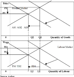
goods and services. This builds a strong ground for the concept of business cycles and unemployment by implying that in seasons of low production due to low demand for goods and services is low demand for labour thus high unemployment and vice versa. In interpreting the classical relationship between demand for products and labour figure 1 links the product market with the labour market. In the figure P stands for price of products, AD is aggregate demand, AS is aggregate supply, w stands for wages, TD is total demand for labour and TS is total supply of labour. It shows that when aggregate demand for products shifts from AD1 to AD2, the demand for Labour also shifts from TD1 to TD2. As a result L1 minus L2 workers lose their jobs due to fall in demand from products from Q1 to Q2 and vice versa. Wages too fall from w1 to w2. Over a given period of time the demand for products fall and rise, consequently the demand for labour fall and rise similarly. This leads to theory of business cycle.

Source: Author

Figure 1. Product and Labour Markets

Theory of Business Cycle and Cyclical Unemployment: There

are four main types of unemployment; frictional, seasonal, structural and cyclical. Frictional results when a person remains jobless while changing from one job to another. Structural unemployment is associated with changes in technology or skills required in production such that people lose jobs due to mismatch of their skills and the market requirement. Seasonal unemployment is associated with opportunities which are periodical such that the demand for labour is low in off-season and high in on-season like jobs at the beaches. Cyclical unemployment is associated with recession and slump, stages of business cycle when demand for products and labour is low, unlike in recovery and boom stages when unemployment reduces. It is cyclical unemployment that Okun (1962) investigated, leading to Okun’s Law. The business cycle is the upwards and downwards swings of the GDP over time emanating from rise and fall in production and demand for products but along a certain growth trend.

About Okun’s Law: Okun’s law states that an increase in real

(1962) who investigated USA unemployment against real GDP over the period 1954-1962. Okun established a relationship which gave the following results; y = 0.30 + 0.30 x: (r2=0.79), where y and x were first differences of unemployment rate and real gross domestic product respectively.

Empirical Literature: A number of studies have investigated

Okun’s Law for various countries. For instance, Bankole and Fatai (2013) found positive Okun coefficient of 0.45 for Nigeria. This led the authors to recommend that the government should concentrate on structural changes and reforms in the labour market; implying cyclical unemployment in Nigeria was insignificant over the period 1980-2008. The study used real GDP and unemployment rate and estimated the relationship using Phillips and Hansen (1990) fully modified ordinary least squares after establishing long run relationship using cointegration test. A study by Hanusch (2012) on 8 countries from East Asia established the following elasticity of employment to changes in real GDP; China (0.30), Hong Kong SAR, China (0.36), Korea, Rep. (0.24), Malaysia (0.39), Philippines (0.22), Singapore (0.42), Thailand (0.33) and Taiwan, China (0.31) over the period 1997 and 2011. The author concludes that the growth in East Africa countries was not jobless since increase in real GDP by 1 percent was associated with increase in employment by between 0.2 and 0.4 percent.

Kamgnia (2009) investigated the growth intensity employment, for 39 countries in Africa covering 1995-2000 period. The study used autoregressive distributed lag panel model with fixed effects and established significant 0.36 elasticity of employment to growth in real GDP and in the presence of foreign direct investment, openness, and credit to the private sector variables which were also significant. A further analysis of the long run effect of lagged real GDP only on employment the author found multiplier 0.25 effect meaning 1 percent increase in GDP absorbs 0.25 percent more labour force. The study concludes by advocating for expansion in output to impact on employment. Ball et al (2012) found Okun’s coefficient of -0.41 for USA using 1948-2011 annual data. The authors also investigated the Okun’s coefficient of advanced economies over the period 1980-2011 countries respective coefficients as follows; Australia 0.54, Austria 0.14, Belgium 0.51, Canada 0.43, Denmark 0.43, Finland -0.50, France -0.37, Germany -0.37, Ireland -0.41, Italy -0.25, Japan 0.15, Netherlands 0.51, New Zealand 0.34, Norway 0.29, Portugal 0.27, Spain 0.85, Sweden 0.52, Switzerland -0.23, United Kingdom -0.34 and United States -0.45. The authors observed that Okun’s law was “strong and stable in most countries” though there were different effect of output on employment across countries.

Brazilian economy was found to have had -0.19 and -0.20 elasticity of unemployment to GDP between 1980 and 2013 in the short run and long run respectively, according to Tombolo & Hasegawa (2014). This was estimated from quarterly data. The authors interpret this to rigidity of the labor market to economic growth. Beaton (2010) found Canada’s Okun’s coefficient ranging between -0.16 and -0.23 in the short run and -0.31 and -0.4 in the long run. This study created sample series for structural breaks of unemployment and real GDP for various intervals over the period 1961 to 2009. In comparison with USA the study found coefficients ranging between -0.21 and -0.23 in the short run and -0.35 and -0.44 in the long run. It established that structural instability for both countries.

METHODOLOGY

The relationship between labour and GDP can be linked from the Cobb-Douglas equation. Cobb and Douglas (1928) addressed questions on relative changes and proportions in capital (K) and labour (L) in production using multiplicative combination of the inputs as shown in equation 1 which assumed constant returns to scale a relationship which was improved by Durand (1937) as acknowledged by Douglas (1976). In the equation Q is quantity produced, and ∝andβ are the share or elasticity of labour and capital in the production respectively.

Q=AKβL∝ (1)

Equation 1 can be transformed to be logarithm form such that it can be estimated using linear estimation techniques as shown in equation 2

lnQ=lnA+βlnK+αlnL (2)

lnL=1

αlnQ− 1 αlnA−

β

αlnK (3)

From equation 3 if we assume Q represents gross domestic product, A to be the state of technology and K remains as capital contribution then we can hold the view that Labour (L) can be explained by level of GDP so will unemployment. The study mainly estimates the relation between real GDP and unemployment using the equation 4. In equation 4 we have lumped components for state of technology, capital contribution and other unknown factors that influence employment levels into β₀

lnU_rt=β0+β1lrGDPt+εt (4)

Where

lnU_rt=log of unemployment (U) attimet

lrGDP=log ofrealGDP β₀=Constant

β₁=elasticityifUonchangesinrealGDP εt=errorterm

Analysis and Findings

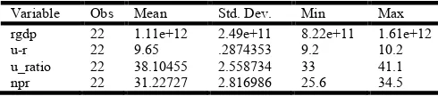
Descriptive Statistics: Over the period 1991 and 2012 the

average real gross domestic product (rgdp) was about 1.11 trillion. Average unemployment rate (u_r) was estimated at 9.65 percent, unemployment ratio (u_ratio) at 38 percent and labor force non participation rate (npr) at 31 percent. Table provides the min, max, standard deviation of the variables.

Table 1. Descriptive Statistics

Variable Obs Mean Std. Dev. Min Max

rgdp 22 1.11e+12 2.49e+11 8.22e+11 1.61e+12

u-r 22 9.65 .2874353 9.2 10.2

u_ratio 22 38.10455 2.558734 33 41.1

npr 22 31.22727 2.816986 25.6 34.5

Test for normality of Data:We test for skewness and kurtosis

rejection of the chi2 are above 0.1 for both series as shown in Table 2.

Table 2. Testing for Normality of Data

Variable Pr(Skewness) Pr(Kurtosis) adj chi2(2) Prob>chi2

lrgdp 0.337 0.126 3.64 0.1622

lu_r 0.902 0.268 1.36 0.5072

Test for stationary: Formal test of nonstationarity using unit

root test as presented in table 3, Augmented Dickey Fuller test, indicate that the log of unemployment and log of actual real gross domestic product at level are non stationary but after first difference they both become stationary, thus the series are integrated of the same order 1, candidates for cointegration as shown in Table 3.

Cointegration and Error Correction Model: Since the series

are integrated of order 1 it creates a necessary condition for cointegration. Cointegration is a process that investigates whether the series which are non stationary at individual levels have a long run relationship meaning a linear combination of the series is stationary. However, by running cointegration we lose the long term relationship thus should advance our analysis to estimate error correction model which will provide the long run relationship and the speed of adjustment of short term deviations to the long run equilibrium.

Testing for Cointegration: The first precondition of

cointegration is fulfilled, that the series lu_r and lrgdp are integrated of the same order. However, this is a necessary but not sufficient condition for cointegration. We conduct a two stage Engle-Granger test of cointegration by running a linear regression in the first stage and then extract the residual of the fitted values which we test for unit root in the second stage.

The first stage regression was conducted and the results were as shown in Table 4. Post estimation test were conducted including test for heteroscadasticity and serial correlation before moving to second stage of EG. We failed to reject the null hypothesis that the series were homoscedastic as shown in Table 5 but both white test and Breusch-Pagan and Cook Weisburg failed to reject the null. Secondly, serial correlation was tested using Durbin Watson (DW) test and as shown in table 5, the computed DW lied between zero and the lower boundary of DW concluding the presence positive correlation between the series and the error term. This therefore, informed the estimation of an OLS while controlling for serial correlation whose results are presented in equation 4. The residual generated from equation 4 were tested for unit root to test for sufficiency condition of cointegration as shown in table 6 cointegration was confirmed between the two variables since the residuals did not exhibit unit root.

_ = 5.55 − 0.12 + Equation 4

− ) (22.95) (−13.60) With R2=0.9069, n=21,

DW=2.49

The cointegration estimation results in equation 5 showed that the cointegration coefficient - 0.55 for the residual was significant and negative as we expected and meaning that in the short run half of the errors causing deviation of the unemployment from the equilibrium in the year (t-1) are recovered in time (t). This is a first recovery mechanism.

dlu_r= −0.006+0.035dlag_lrgdp−0.55lag_residual Equation 5

P>t (0.002) (0.469) (0.008)R2 = 0.3555, n = 20

Table 3. Test for Stationarity of Data

Augmented Dickey Fuller Test Critical Values: -3.750 at 1%, -3.000 at 5% and -2.630 at 10% ADF Test Statistic Z(t) P(t)-Z(t) H0: has unit root

Levels lunemp_rate -1.104 0.7135

largdplcu 2.428 0.9999

Differencing dlunemp_rate -7.674 0.0000

dlargdplcu -3.268 0.0164

Table 4. First Stage Engle-Granger Cointegration Test

First stage OLS

lunemp beta t n = 22

largdplcu -0.13 -17.67 R-squared = 0.9398

constant 5.97 28.51

Table 5. Testing for Heteroscedasticity and Serial Correlation

Table 6. Second Stage Engle-Granger Cointegration Test

Second stage: Unit root status of residual of first stage Augmented Dickey Fuller Test (ADFTest) H0: series has unit root

ADF Test Statistic Z(t) 1% Critical Value 5% Critical Value 10% Critical Value P(t)-Z(t)

-4.207 -3.750 -3.000 -2.630 0.0006

Testing for Serial correlation and Heteroscedasticity Test for Serial correlation (Durbin Watson Test)

Lmin + SC dl Inconclusive du

Fail to Reject

Null 2

Fail to Reject

Null

4-du Inconclusive 4-dl - SC Lmax

0 0.87 1.22 1.42 2.58 2.78 4

Test for heteroscedasticity (White test and Breusch-Pagan / Cook-Weisberg test

White Test H0=homoscedasticity Prob > chi2 = 0.2435

Error Correction Model: We now estimate error correction model to recover the long run relationship. Equation 6 shows that almost 40 percent of the errors generated in time, t-1, causing deviation of unemployment from the longer equilibrium are cancelled in time t.

The long run relationship in equation 7 indicates that an increase in real GDP by 1 percent reduces 0.12 percent unemployment. Therefore, 10 percent increase in real GDP has potential of reducing unemployment by just 1 percent.

Short run error correction mechanism

D_lu_r = − 0.38_ce1L1 − 0.49lu_rLD + 0.058lrgdpLD −

0.013 Equation 6

P>|z| (0.027) (0.015) (0.217) (0.000) R2 = 0.7372 n = 20

Cointegration equation

_

Forecasting: Implication of the Results

Okun’s Law partially holds in Kenya, this is because the negative relationship between unemployment rate and real GDP is upheld but not its magnitude. An increase in real GDP by 10 percent and not 3 % leads to a reduction in unemployment rate by 1%. Further, the percentage change in real GDP that are targeted in the MTP II can therefore be used to estimate the expected respective targets of unemployment rate based on our results. Factoring in the 0.12 percent reduction in unemployment rate associated with an increase in real GDP by 1 percent gives us the resultant change in unemployment rate, which is computed by multiplying the target in percentage change of real GDP with Okun’s Coefficient. Unemployment rate target for 2017/18 is 3.38 percent down from 9.24 percent in 2012, realized only if the economy grows at the targeted rates of real GDP. It will therefore take Kenya at least 5 years to achieve at least 4 percent unemployment rate going by the MTP II real GDP targets, as shown in table 7, ceteris paribus. Alternatively, it is possible it will take Kenya at least 10 years to achieve 4 percent unemployment rate if we by 4.5 percent constant growth rate of real GDP resulting in 0.54 reduction in unemployment per year given our Okun’s coefficient with the year 2012 being the baseline whose actual rate of unemployment was 9.24 percent, ceteris paribus. Therefore, we can feasibly conclude that 4 percent is within the vicinity of Kenya’s achievable unemployment rate projected from the computed 3.38 unemployment target for the year 2018 with 10.6 percent growth rate in real GDP.

In order to achieve this forecast of unemployment rates, growth in real GDP would require doubled investment (capital), land use and technological progress. Therefore, increased private investment (domestic and foreign),

consumption and government spending will be critical. Though it is strategic to identify flagship sectors, as has the MTP II done by picking seven sectors, such sectors should not be construed as the only carriers of the country’s growth destiny.

This will compromise the desired rates of unemployment since they will alienate labour force due to their skills making structural unemployment drag efforts reducing cyclical unemployment. Multi-sector approach to growth as a strategy against unforeseen shocks and is critical. In the short run fiscal policy instruments are highly advocated for given that Kenya is a developing economy. The desire to grow the economy yet the sectors earmarked are capital absorbing than they are labour absorbing will hinder achievement of the predicted cyclical unemployment.

Conclusion and Recommendations

Conclusion

It has been established that Okun’s law partially holds in Kenya with negative sign but different magnitude. It is a 10 percent increase in real GDP and not 3 percent which would cause 1 percent reduction in unemployment rate. As a result, given the MTP II targets of real GDP for the period 2012-2018, Kenya has potential to achieve 4 percent unemployment rate within the 5 year period having taken into account the recorded unemployment rate of 9.24 percent in the year 2012, our base year, and the estimated Okun’s coefficient of 0.12 However, it will take Kenya at least 10 years to reach the predicted 4 percent unemployment rate if it continues to consistently grow at 4.6 percent as recorded in 2013 which results in 0.54 percent annual decline in cyclical unemployment.

Recommendations

Going forward the study recommends that Kenya government should consider the following as critical areas to inform action on controlling cyclical unemployment using economic growth macroeconomic policy.

 Target to achieve 4 percent cyclical unemployment rate by 2018 but if this target is missed then the year 2022 should be the worst timeline. This will enable the county set strategies to sustain the achievement running stable towards the year 2030.

 In order to achieve the recommendation in (i) strategies need to be put in place or the existing strategies be strengthened to control structural and seasonal unemployment which are all involuntary. Such strategies should consider balancing flagship sectors that are earmarked to drive growth with respect to their propensity to substitute labour for capital. Otherwise with massive investment and focus on such flagship sectors unemployment rate will increase if the efforts

Table 7. Forecasting on Unemployment Rate Targets for 2012-2018

2012 2013 2014 2015 2016 2017 2018

Target % change in Real GDP per MTPII 4.5 5.4 6.7 7.8 8.7 9.6 10.6

Resultant Change in Unemployment Rate (Computed Based on Results) 0.54 0.65 0.80 0.94 1.04 1.15 1.27

Unemployment rate target 9.24 8.59 7.79 6.85 5.81 4.66 3.38*

NB: 3.38* opens vicinity of 4 percent unemployment rate target for 2018

are skewed to capital intensive technologies and season prone unemployment sectors.

 Given the low Okun’s coefficient of 0.12 for Kenya it will be strategic to encourage as a minimum, a 10 percent growth in consumption, investment (capital growth) and government spending from each previous year to cause at least 1 percent reduction in unemployment. This should be the threshold multiplier of factors of production and technology to spur threshold real GDP cause the estimated effect on unemployment rate.

REFERENCES

Ball, L., Leigh, D., & Loungani, P. 2012. Okun’s Law: Fit at 50? Laurence Ball; Danie13th Jacques Polak Annual Research Conference November 8–9. International Monetary Fund. Bankole, A. S., & Fatai, B. O. 2013. Empirical Test of Okun’s

Law in Nigeria. International Journal of Economic Practices

and Theories, Vol. 3 (No. 3), e-ISSN. 2247–7225.

Beaton, K. 2010. Time Variation in Okun's Law: A Canada and U.S. Comparison. Ottawa, Ontario: Bank of Canada.

Cantillon, R. 1730. Essay on the Nature of Trade in General. London: Frank Cass and Co., Ltd.

Cobb, C. W., & Douglas, P. H. 1928. A Theory of Production.

The American Economic Review, Vol. 18(1), pp. 139-165.

Douglas, P. H. 1976. The Cobb-Douglas Production Function Once Again: Its History, Its Testing, and Some New Empirical Values. Journal of Political Economy, Vol. 84(5), pp. 903-916.

Durand, D. 1937. Some Thoughts on Marginal Productivity, with Special Reference to Professor Douglas' Analysis. Journal of

Political Economy, Vol. 45(6), pp. 740-758.

Government of the Republic of Kenya. 2013. Second Medium Term Plan, 2013 – 2017; Transforming Kenya: Pathway to Devolution, Socio-Economic Development, Equity and National Unity. Nairobi: Government of the Republic of Kenya.

Government of the Reublic of Kenya. 2003. Economic Recovery Strategy for Wealth and Employment Creation. Nairobi: Government of the Reublic of Kenya.

Hanusch, M. 2012. Jobless Growth? Okun’s Law in East Asia. Policy Research Working Paper 6156: The World Bank. Kamgnia, D. B. 2009. Growth Intensity of Employment In Africa:

A Panel Data Approach. Applied Econometrics and International Development, Vol.2 (No.2).

Marx, K. 1867. Critique of Political Economy. Verlag von Otto Meisner.

Okun, A. 1962. Potential GNP: Its Measurement and Significance. Proceedings of the Business and Economic Statistics Section of the American Statistical Association. Yale University: Cowles Foundation.

Smith, A. (1776). An Inquiry into the Nature and Causes of the Wealth of Nations. London: W. Strahan and T. Cadell. Tombolo, G. A. and Hasegawa, M. M. 2014. Okun's Law:

Evidence for the Brazilian Economy. Munich Personal RePEc Archive.

World Bank. 2014. World Bank Open Data. The World Bank Group.