Active bandsaw control

(1)

Active Bandsaw Control

RaCleave

A thesis presented for the degree of

Doctor of Philosophy

in

Mechanical Engineering

at the

University of Canterbury,

Christchurch, New Zealand.

(2)

(3)

ABSTRACT

This thesis investigates the modelling and active control of narrow and wide band-saw blades, with application to the band-sawmilling industry. Strings, beams and plates are considered in the modelling work, with advances made in the modelling of ex-ogenous influences and multispan saw blades. Beams and plates are considered in the control work, with classical and optimal controllers considered. Importance is placed on closed-loop robustness with respect to parametric variation, closed-loop performance in vibration suppression and in providing a physically realisable solu-tion to the control problem.

In the string and beam work exogenous influences are modelled by pointwise and distributed forces, including; lateral stiffness, lateral damping and a "follower" force that comprises an in-line and a lateral component. Pointwise actuation and ar-bitrary disturbance forces as well as pointwise sensing are also included. Successful comparison with results of other contributors, as well as comprehensive experimen-tal work, validates the modelling. The experimenexperimen-tal validation also concentrates on system damping and the integration of sensing and actuation.

The plate work considers the single-span cutting blade presented by other con-tributors, and extends it to include saw guides and partial-span cutting forces. These cutting forces include damping, stiffness and follower loads, and act over a partial length of the cutting edge. While this three span model is not experimentally veri-fied, it is shown to produce credible results.

The control work is in two parts. A comprehensive study of the robustness of various controllers with respect to translation speed and band tension is performed for the beam; theoretically and experimentally. The theory-practice gap was small regarding trends in robustness, but unmodelled effects such as the band weld de-graded the agreement of absolute values at higher band speeds. Classical controllers were abandoned due to high frequency noise amplification, and a near optimal1ioo loop shaping controller was found to be superior to others of its type and various 1{2 formulations. The plate work is entirely theoretical, but uses the same actuator and sensor dynamics that were successful in the beam work to maintain the phys-ical feasability of the controllers. Both single span and multispan systems are con-sidered, with the central cutting span of the blade being controlled via actuation

(4)

and sensing of the upstream and downstream noncutting spans. Robustness stud-ies were conducted, with satisfactory robustness achieved with respect to a .large number of parameters. Furthermore, substantial increases in maximum allowable cutting loads were achieved, as well as reduced vibration energy.

(5)

ACKNOWLEDGEMENTS

First and foremost I extend my thanks and appreciation to Dr Christopher Damaren. my mentor and supervisor. His enthusiasm for engineering science, dedication as a supervisor and knowledge of the subject have been invaluable and inspirational to me.

I also thank Emeritus Professor Harry McCallion for his humour, approachability and ability to ask the trickiest of questions.

This work would not have even started without the ongoing work of Dr Lan Le-Ngoc from Industrial Research Limited. Dr Le-Le-Ngoc's technical support and advice throughout the entirety of my research, and continual supply of equipment has been greatly appreciated.

Dr Ian Huntsman I thank for taking over my supervision when Dr Damaren left the University. His encouragement as well as his checks on my progress were both welcome and effective.

Throughout this work my closest technical colleague has been Andrew Cree. The many discussions about controls implementation and problems thereof were irre-placeable. Andrew is also responsible, in his role as a departmental technician, for designing and building much of the specialised electronic equipment and software I required in this work.

To my office mates and true compatriots Sue Wilkinson and Charles Breurkes I extend huge thanks. I shall always keep with me the shared memories of coffee breaks, frustrating times, successful times and times when the brain simply felt too fulL Also, thanks to Jonathan Harrington for years of late night discussions and cups of tea.

For their financial support I would like to thank the Department of Mechanical Engineering at the University of Canterbury, Industrial Research Limited in Christ-church, New Zealand and the Todd Foundation of Todd Energy, New Zealand. With-out such support this work could never have been done; I now look forward to the time when I can be part of an institution that supports such efforts.

(6)

(7)

LIST OF FIGURES

1.1 Modern bandmill.

1.2 Bandsaw tooth parameters. 2.1 The translating tensioned string.

2.2 Stationary mass-spring-damper system attached mid-span. 2.3 Phase propagation in the first and second modes of vibration.

2 3 8

10

21 2.4 Approximate and exact frequencies versus speed for a translating string. 21 2.5 Approximate frequency versus speed for a translating string. 22 2.6 Effect of distributed damping on vibration frequencies for the moving

string. 24

2.7 Distributed follower load and corresponding lateral component. 25 2.8 Effect of lateral component of the distributed follower force on

vibra-tion frequencies for the stavibra-tionary, untensioned beam. 25 2.9 Modal forms of the first two modes of the stationary untensioned beam

as lateral follower load increases. 26

2.10 Effect of distributed follower load on vibration frequencies of the

sta-tionary beam. 27

2.11 Effect of pointwise spring force and damping on vibration frequencies

for the moving string. 28

2.12 Effect of pOintwise follower load on vibration frequencies for the

mov-ing strmov-ing. 28

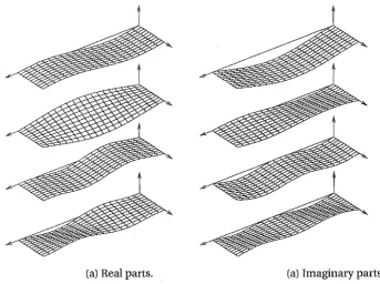
3.1 Modal precession for first four natural modes of vibration, C = ~CC1' 34 3.2 Deflections arising from the real and imaginary parts of the

eigenvec-tors of the first four modes of vibration, C

!c

_cr 35 3.3 Plate end loads created by blade tensioning, wheel crown and wheel tilt. 36 3.4 Effect of varying the linear stress variation across the width of the plate. 36 3.5 Modal forms and nodal lines for the first four modes for the tensioned

(12)

3.6 N,7: and N.7:Y for a constant cutting load. 38 3.7 Effect of in-plane component of the distributed follower force on the

stationary plate. 40

3.8 Mode shapes for tangential component offull-spanfollower load, kf

15kN/m. 40

3.9 Change in imaginary parts of eigenvalues for increasing full-span

cut-ting load. 41

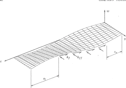
3.10 Form of partial cutting load, showing tangential follower force and

normal feed force. 42

3.11 N.T,N.7:Y'Ny for a constant cutting load acting along a partial span of

the leading edge (su

=

0.3£, Sl = 0.2£). 45

3.12 N.7:' N.7:y, Ny for a constant cutting load acting along the entire length

of the leading edge (S1L = 0, Sl = 0). 46

3.13 Modal forms using partial cutting formulation for cutting along the

entire leading edge. k f

=

15kN / m 47

3.14 The effect of increasing the number of terms in the Fourier

represen-tation of the cutting load. 47

3.15 Effect of distributed cutting edge stiffness on vibration frequencies for

the moving plate. 49

3.16 Modelling guides by areas of restitutive pressure. 53 3.17 The effect on vibration frequency of the cutting span length. 53

3.18 Modal forms of the single and three span blades. 54

4.1 Bandsaw rig and associated hardware. 58

4.2 Bandsaw rig - elevation. 58

4.3 Generic B -H curve for ferromagnetic material 59

4.4 Generic hysteresis loop for ferromagnetic material. 60 4.5 E-type electromagnet, showing the core area, A e, and side areas, As, of

the face. 61

4.6 Experimental frequency response of stationary beam. 63 4.7 Experimental and theoretical frequency responses of a stationary beam. 64 4.8 The effect of blade tension on experimental and theoretical frequencies. 64

4.9 Experimental and theoretical Bode plots of a moving beam. 'fJ

=

1,

c

=

15m/s. 65

4.10 Comparing the effect of blade speed on experimental and theoretical

frequencies. 66

(13)

LIST OF FIGURES xiii

4.12 Experimental and theoretical frequency responses of a plate. 68 4.13 Experimental plant compared with damped theoretical plant. 'f} =

1, c = 15m/s. 70

4.14 Experimental plant compared with theoretical plant augmented with

second order actuator dynamics. 71

5.1 SISO electromagnetic feedback control of translating continua. 78

5.2 General block diagram of SISO feedback control. 78

5.3 General feedback problem. 80

Lower LFT diagram of feedback control. 81

5.5 Bode plot of simple rate feedback controller in series with 2 mode

string model. 83

5.6 Impulse response of closed loop with simple rate feedback controller 83 5.7 Bode plot of simple rate feedback controller in series with 4 mode

string model.

5.8 Bode plots of rate feedback controllers. 5.9 Noise sensitivity of two classical controllers. 5.10 Bode plots ofLQG/1-£2 and classical controllers.

84 85 86 92 5.11 Noisy impulse response for 2 mode stringmodelin feedbackwithLQG/1-£2

controller. 92

5.12 Noisy impulse responses for LQG /1-£2 control of nominal and perturbed

stationary string. 93

5.13 Unstructured uncertainty descriptions. 95

5.14 LFT showing uncertainty block, plant and controller. 96 5.15 Singular values for shaping function and open loop systems for the

string example. 100

5.16 Impulse responses of string in feedback with 1-£00 controller 100 5.17 Performance specifications for classical controllers. 103 5.18 Performance specifications for 1-£2 controllers. 104 5.19 Performance specifications for 1-£00 controllers. 104 5.20 Controlled impulse responses of stationary beam (First plot). 106 5.21 Controlled impulse responses of stationary beam (Second plot). 107 5.22 Free responses of moving beam, subject to four disturbances. 110 5.23 Speed robustness of controlled responses of LQG1, HINFl, HINF2,

HINF3 for the impulsive disturbance. 112

5.24 Speed robustness of controlled responses of LQG1, HINF1, HINF2,

(14)

5.25 Speed robustness of controlled responses of LQG1, HINF1, HINF2,

HINF3 for sinusoidal disturbance. 114

5.26 Speed robustness of normalised controlled impulse responses ofLQG2

and LQG2b. 115

5.27 Tension robustness of controlled responses ofLQG1, HINFl, HINF2,

HINF3 with impulse disturbance. 116

5.28 Tension robustness of controlled responses ofLQGl, HINF1, HINF2,

HINF3 with sinusoidal disturbance. 117

5.29 Comparing the position of the sinusoidal disturbance on the

perfor-mance ofLQGl, HINF1, HINF2, HINF3. ll8

5.30 Speed robustness of normalised controlled random responses ofLQGl

and LQGla. 119

5.31 Free responses of moving beam, subject to three disturbances. 119 5.32 Speed robustness of constrained wheel problem, controlled responses

of LQG 1, HINF 1 and HINF3 for the impulsive disturbance are shown. 120 5.33 Speed robustness of constrained wheel problem, controlled responses

of reduced versions ofLQGl, HINFI and HINF3 for the impulsive

dis-turbance are shown. 121

5.34 Robust stability for rj

=

1 with respect to speed, for both the beam and

plate problems. 122

5.35 Robust performance for HINFI and HINF2. 123

5.36 Sketch of plate model proposed in Damaren and Le-Ngoc (2000). 124 5.37 Root loci as full length follower load varies from kf 0 to kf -50kN Im.125

5.38 Impulse response under cutting conditions. 125

5.39 Root loci of the first ten modes of the full order model with respect to

cutting load. 126

5.40 Bode and maximum singular value plots ofLQG controller. 127 5.41 Root loci of plants produced by various reduction procedures. 128 5.42 Bode plots of plants produced by various reduction procedures. 130 5.43 Impulse responses for an idling saw, showing the effect of the restraint

of the cutting edge. 131

5.44 Root loci for complex damping formulation. 132

5.45 Modal forms of complex damping modeL 133

5.46 Idling and cutting impulse responses for complex damping model. 134 5.47 1-l2-norms of performance output of the single span saw with respect

to cutting load and tension. 137

(15)

LIST OF FIGURES

5049 Maximum singular value plots ofLQG controller.

5.50 Modal forms of restrained but noncutting multispan system.' 5.51 Stress state of multi span blade.

5.52 1-l2-norms of performance output for the multispan saw with respsect

xv

138 140 141

to cutting load and tension. 143

B.l Static analysis. 155

B.2 Rig for determining magnet force-distance-current relationship. 157 B.3 Static magnet calibration using steel block as target. 158

BA Input and output curves for magnet calibration using steel block as

target. 158

B.5 Frequency response for electromagnet over 2000 rad/s. 159 E.G Hysteresis curves at different forcing frequencies. 159 B.7 Static calibration of electromagnet using tensioned beam. 161 B.8 Calibration at different nominal distances, using saturated analysis. 162 B.9 The effect on the position measurement due to four different

mag-netic fields.

E.lO The effect on the position measurement due to sinusoidally changing magnetic fields.

B.l1 Noise signal and corresponding spectra. C.1 Coprime factor uncertainty.

C.2 LFT showing uncertainty block, plant and controller. C.3 Measuring open loop uncertainty.

CA Measuring closed-loop uncertainty. C.5 TWo connected carts.

163

163 163

171

(16)

(17)

LIST OF TABLES

2.1 Nominal parameters for results of Chapter 2.

3 .1 Natural frequencies for a plate that is simply supported on two oppo-site boundaries and free on the other two.

3.2 Nominal parameters for results of Chapter 3. 4.1 Bandsaw rig specifications

4.2 Electromagnet specification

5.1 Bandmilling uncertainties

5.2 Closed-loop performance specifications

20

34

39

59

61

77

Sl

5.3 String parameters. S2

5.4 Controllers for experimental beam analysis. 103

5.5 6,.1 metric for beam model as translation speed changes from c =

ami

s

to c = 60ml s. lOS

5.6 51.! metric for beam model as blade tension changes from Ro 160N

to Ro = 400N. 109

5.7 51.! metric for beam model as translation speed changes from c Oml s

to c = 60ml s. 109

5.S Effectiveness of LQG I controller with respect to variations in the band speed used in synthesis and analysis, as measured by IIyl12 x 103• III

5.9 Effectiveness of LQG I controller with respect to variations.in the band tension used in synthesis and analysis, as measured by IIYl12 x 103• 115

5.10 Model reduction schemes used in plate analysis. 129

S.1I 1£z-norms for impulse responses of single span blade. 135

5.12 Performance measures and stability margins for single span. 136

5.13 1£z -norms of impulse responses for 1£2 controlled multispan blade. 139

5.14 1£z-norms of impulse responses for 1£00 controlled multispan blade. 142

5.15 1£z -norms of impulse responses for 1£2 and 1£00 controlled multispan

(18)

C.1 lin ( Ot 1 G j) for two cart system (Example D. 176

C.2 0/1 ( Gi , G.1) for two cart system (Example D. 177

C.3 ()n ( Oi 1 G_{j )}for two cart system (Example II). 177

C.4 il/I (Gi, o.j) for two cart system (Example II). 177

C.S On ( 0;, 1 OJ) for two cart system (Example lID. 178

(19)

Chapter 1 INTRODUCTION

1.1 BAND SAWS

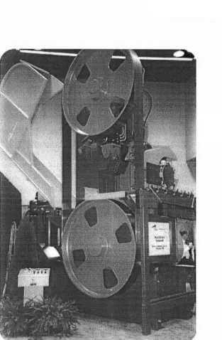
Bandsaws, or more properly, bandmills, are the most common machine used to pro-duce boards from logs in the sawmilling industry. The first saws were built in the mid 1800s but produced unsatisfactory lumber in comparison to sash saws and circular saws. The 1880s saw some earnest yet ad-hoc developments and soon after this time bandsaws superseded circular saws as the most common means of cutting logs. A bandmill comprises the structure and machinery required to strain, drive and track a bandsaw, which is the continuous loop of steel that actually cuts the timber. A modern example is pictured in Figure 1.1. Logs are fed through the saw using feed machinery. For a thin band of steel to remain on the band wheels it must be under some strain. The mechanism that provides such strain is the most important part of a bandmill, as this maintains blade position in the face of varying cutting loads, feed loads and operating speeds.

Bandmill strain. Throughout much of the 1900s blade tension was maintained by pivoting the top wheel shaft on a rocker arm, with the weight of the wheel assembly reacted by a linkage attached to an arm and mass arrangement. This simple coun-telweight mechanism worked well but lacked mechanical damping (aside from fric-tion), and was replaced in the 1970's by air-strain mechanisms that reacted the wheel assembly mass using compressed air. The compressed air improved damping char-acteristics and removed the inertia of the hanging weights, thus improving response times. Since then actively controlled hydraulic systems have evolved, further im-proving dynamic response and damping.

(20)

[image:20.597.172.485.150.628.2]

(21)

1.1 BANDSAWS 3

axis of rotation. Such wheel tilting does improve saw tracking, but is most commonly used when the saw tensioning (defined below) has become unsatisfactory.

Handsaw. The bandsaw itself has also received technological attention over the years. The major factors affecting bandsaw performance are the "set" of the teeth and the tensioning of the blade. Initially bandsaws were made with offset teeth (called "spring set"), however this was soon replaced with swage set teeth, which are symmetrical about the centre plane of the blade but flared so that the tooth width, or kerf width, is larger than the blade thickness. In the early 1980s tipped teeth were being used and now most large bandsaws use stellite tipped teeth, which offer bet-ter wear resistance but must be welded onto the blade. The cutting edge is heated more than the trailing edge during operation, and the lengthening caused by this heating is offset by lengthening the trailing edge prior to use. This is in addition to a lengthening of the middle width to fit the crowning of the band wheels. Such rela tive lengthening is termed "tensioning" in the art of saw-doctoring.

Figure 1.2 defines some of the parameters involved in the cutting teeth. The gullet size is also important to blade stability. Gullets that are too small fill with saw dust quicldy, and "clumps" of excess dust get forced between the side of the blade and the sawn timber, creating unwanted lateral loads.

Guides. Bandsaws usually have two guides, one on either side of the workpiece. For increased saw stability they are placed as close as possible to the workpiece, and the top guide is often adjustable sometimes automatically

so.

Thin bandsaws of-ten use roller guides, while wide bandsaws use low friction, wear resistant materials. The guides enact a constant lateral pressure to the blade so the cutting span is offset from the line joining the band wheels. Some guides are lubricated, with the trans-lation of the blade over the oil film creating a fluid bearing. Some saw millers quote superior performance without guides; however this is not the norm.

Pitch

f3 ack of looth

Face of tooth

Hook

(22)

Wijesinge (1998) is an excellent reference containing introductory, historical and operational information on the bandmill and bandsaw.

1.2 ANALYTICAL TREATMENT OF AXIALLY MOVING CONTINUA

Not until the pioneering work of Mote in 1965 did analytical science enter the previ-ous century of ad-hoc optimisation that bandsaws had undergone. Mote's work was seminal in the wide bandsaw arena but relied upon the work of Skutch (1897) which was the first theoretical investigation of axially moving continua. Mote has been a principal author up to the present day, with other notable contributors being Nag-uleswm"en, Ulsoy, Wickert, Wang, Okai, Kimura, Yokai, Lengoc, McCallion, Lehmann and Hutton. Full literature reviews are presented in Chapters 2 and 3.

Work on the active control of axially moving continua has been considered since the late 1980s, with a large number of authors contributing over this time. A full literature review of this work is given in Chapter 5.

1.3 MOTIVATION FOR FURTHER IMPROVEMENT

From the foreword in Wijesinge (1998), typical yields of the British Columbian sawmilling industry in 1968 were approximately 40% (from log to finished product). By 1972 this figure was 53.3%, and today yields of 70% are required to remain competitive. In contrast, yields in tropical countries throughout Africa, Asia and Latin America are currently around 40-55% (Loehnertz et al., 1994). As well as high yield, high through-put is of major concern to saw millers. A limiting factor to high throughthrough-put is the speed with which logs and boards can be fed through the machines (known as the feed rate or speed) before saw stability is compromised. Also, machine down times reduce throughput, so long blade and guide lives are important.

To improve yield and throughput, the following may be reduced:

.. Kerfwidth. Thinner kerfs obviously mean less waste, and is limited by the al-lowable stress of the blade and teeth. In aeronautical and other high cost mar-kets kerf becomes especially important.

(23)

1.4 CHAPTER PRECIS ₅

" Snake. This is a low frequency "snaking" of the blade along the length of the log or board, again producing excess waste.

" Snipe. A sudden change in blade position at the start or end of the cut, requir-ing the removal of the ends of boards.

• Wedging. This is a change in blade position throughout the depth of the cut, causing wedge shaped boards and again increased waste.

These phenomena are all related to blade stability, so increasing blade stability increases yield. This is the major motivation for this research into the active control of sawblade vibration.

1.4 CHAPTER PRECIS

1.4.1 Strings

and

Beams

Hamilton's principle is applied to the kinetic, potential and non-conservative en-ergies of the travelling string. The string is subjected to distributed and pointwise cutting and actuator forces, and the deflection is discretised using the method of Ritz. Pointwise sensing is also discussed. Material stiffness is then added and re-sults for both the string and beam given. This work is not new but formulates and solves the string problem in detail, and combines and compares the work of other contributors.

1.4.2 Plates

(24)

1.4.3 Experimental apparatus

This chapter develops a noncontacting collocated actuator-sensor, and uses it to validate the string, beam and plate models. The actuation is electromagnetic, and provides the first step toward an industrial solution. The validation work is com-prehensive, covering speed effects, bandmill tension, damping and actuator-sensor dynamics. The damping and actuator-sensor work is particularly important to the ensuing control work.

1.4.4 Control

Investigation of the active and passive control of axially moving continua first re-ceived attention in the late 1980s, and the work to date is summarised. This work focuses on the active control of bandsaws, using modem, model-based controllers. The bandsaw problem is cast as a control problem, and the required control theories discussed with continual application to the bandmilling arena. This work focuses on using lateral control to further stabilise the blade; this is a matter of project scope and potential application to other fields. Further improvements to current strain mechanisms, including activation is of course feasible, but not considered here.

(25)

Chapter 2 STRINGS AND BEAMS

The vibration of axially moving continua has been studied for over a hundred years, beginning with strings and progressing to beams and plates. Applications are tape ribbons, belts, pipes containing flowing fluids, power transmission chains and belts, aerial cable ways and bandsaws. This chapter formulates linear finite-dimensional models for translating strings and beams that are subject to exogenous influences, and examines the resulting behaviours. The exogenous influences describe effects such as forces from read/write heads on magnetic tapes, cutting forces on bandsaw blades and control actions.

Skutch (1897) was the first to solve the moving string problem, and since then many have contributed to the area. The effect of translation upon vibration frequen-cies and modal forms was first considered using linear theory and then using non-linear methods. Thorough reviews of the literature may be found in Mote (1972), Wickert and Mote (1988), and references here will only be made that are pertinent to the discussion at hand. Miranker (1960) showed that there exists a periodic trans-fer of energy into and out of the span of a travelling string, and Mote and Wickert (1989) quantified this energy transfer for various boundary conditions. Because this transfer is of second order in the lateral component of the translation of the string it is ignored throughout this treatment. Exogenous influences first received atten-tion in 1967 by Alspaugh, who considered the torsional vibraatten-tion of a moving strip· under the influence of a pointwise edge load. Also, the effect of read-write heads on magnetic tapes was considered by Ono (1979), and later Chonan (1986) consid-ered a moving strip subjected to a stationary lateral load system. Wickert and Mote (1990) provided a general solution to axially moving strings subjected to arbitrary but mathematically tractable lateral loads.

(26)

formu-lation and solution of motion equations is detailed in this chapter but omitted in the next.

2.1 THE TRANSLATING STRING

Figure 2.1 shows a tensioned string translating at speed c between two frittionless guides and vibrating in the wx-plane. The string has mass density p, cross-sectional areaA, is laterally loaded by a distributed force fw(x, t), and is under tension R(x, c, t)

whith varies due to in-line loads fx(x, t) and the transport speed c.

fw (x, t )'-r---r--1.

x

(x, t)

R(O, c, t) _p,A

Figure 2.1: The translating tensioned string.

~

R(i, c, t)

Hamilton's principle may be used to generate motion equations for the various systems considered. Hamilton's principle states that the true motion of a conserva-tive system throughout the interval of time [tIl t2J is such that the integral

(2.1)

is rendered stationary. Here I:- = T - V is called the Lagrangian, and is the differ-ence between the system's kinetit energy,

T,

and its potential energy, V. The kinetit energy is assumed to depend on the positions and velocities of the components of the system, whereas the potential energy depends only upon the positions. If the position of the system can be uniquely specified by as many geometrical quantities as there are degrees of freedom for the system, then the Lagrangian may be written in terms of these quantities, which are called generalised coordinates of the system.

(27)

neigh-2.1 THE TRANSLATING STRING 9

bouring motions must be zero. Then, Hamilton's principle may be expressed as

(2.2)

where JT and JV are variations (with respect to neighbouring motions) in the ki-netic and potential energies of the system. In nonconservative systems Hamilton's

extended principle, which includes the virtual work done by nonconservative forces,

is used. This may be written as

(2.3)

where JWnc is the virtual work done on the system by nonconservative forces. In

the development below the conservative work caused by exogenous lateral forces is combined into the virtual work term, rather than into the potential energy. This is to clarify the development, and so henceforth this term shall be labelled JWex • Once

expressions for the system energies and virtual work are found, (2.3) may be solved to find the governing equations of motion.

2.1 Kinetic and potentiaillJln& .... O'I

The velocity of an element of the moving string comprises components from the

:D- and 'W-directions. The lateral ('Ill-direction) component arises from the instanta-neous vibration velocity, a'W j at, and the 'w-component of the transport velocity of the string, c(a'Wjax). The x-component comes from the translation speed c, and thus the kinetic energy

T,

may be written as

T

₂1

j

0 .e pA [ c 2

+

(a

at

'W

+

c

a)

ax 'W

2J

dx. (2.4)

The absence of material stiffness in a string means the strain due to vibration is sim-ply caused by the length of the string changing. The resulting strain energy is given by

v

=!

1£

R(x,c)

(~:)

2 dx, (2.5)

(28)

2.1.2 Exogenous forces

The work done by exogenous forces fex

=

fw(x, t) in displacing the string by a virtual amount Ow is given by

(2.6)

where expressions for these forces depends on the system being analysed. Figure 2.2

----

R(O,

~

R(e,c,t)

Figure 2.2: Stationary mass-spring-damper system attached m,id-span.

shows a string in contact with a mass-spring-damper located part way along the span. The spring provides a force in proportion to but acting against the deflection at the point of contact, while the damper produces one acting in proportion to but against the lateral velocity of the string. Also, friction caused by the contact forces produces a force in line with and against the direction of travel of the string, which again acts at the point of contact. Follower forces act so that the direction of force follows the slope of the deflected shape. The initial application of this idea was mis-sile stability, where follower forces acting at one end of a free- free beam were used to model thrust force. This follower force has a component in the x-direction, detailed below, and a component in the w-direction which depends upon the slope of the string. Also shown in Figure 2.2 is a time varying force, u(t), acting at x X_{a ,}which

when combined with the other lateral loads gives the exogenous force

(2.7)

where ks, ki and kf are the spring, damping and friction force coefficients respec-tively, and 8(x -Xd) is Dirac's delta function located atxd' Equation 2.7 is a fair model for a contacting passive actuator, or the heads of high speed tape drives. However, more applicable to the sawmilling industry is the situation where the forces act in a

(29)

2.1 THE TRANSLATING STRING 11

distributed fashion along the entire length E. Then (2.7) becomes

lex

(2.8)

with the obvious changes in units of ks ) kd and kf.

2.1.3 Other effects

Variation of tension with speed

Maintaining the tension of wheel and band systems is achieved by a variety of strain-ing mechanisms dependstrain-ing on the application. In bandmills the blade is dynami-cally tensioned through dampened counterbalances attached to the nondriving wheel. This mechanism removes large fluctuations in the tension due to speed changes and cutting influences. Mote (1965) first considered the relationship oftension to speed, finding that

(2.9) which can be explained by the acceleration of the blade moving around the wheels.

For a bandrnill with wheels fixed in space the centripetal acceleration of the blade around the wheels requires a force which reduces the interference pressure be-tween the wheels and the blade. As the overall band length is not changing the ten-sion remains at the initial value Ro. If the interference pressure remains constant (by the use of a counterweight mechanism applied to one wheel) then the centripetal acceleration is reacted by an increase in band tension, this increase being equal to

pAc2• Thus a value of'TJ 0 in (2.9) describes the situation for fixed wheels, while a value of'TJ 1 describes the counterweight mechanism. If a finite stiffness is applied to one wheel assembly then the centripetal acceleration is reacted partially by an in-crease in tension and partially by a dein-crease in the force on the wheel assembly, and so a value of 0 'TJ

<

1 is appropriate. Mote (1965) details calculation of 'TJ given a certain stiffness of the wheel assembly.

Variation of tension along the length

The :l;-component of the follower force discussed in the previous section gives rise to a change in tension along the length, E. This change may be approximated in the distributed loading as a linear increase in tension along the length, and in the point-wise loading as a step change at x

=

Xd. For a simple counterweight mechanism the

(30)

load must be reacted by an increase in the tension at the downstream (x f) bound-ary, which is supplied by the drive motor. So, the tension at x 0 (the nondriving end) increases from the nominal value Ro

+

pAc2 to Ro

+

pAc2

+

kf at x = f. If the strain mechanism is an air strain or clamped system, then the blade tension at the un driven pulley boundary may vary, and thus the cutting force may reduce the ten-sion at this boundary. The drive motor must still react the cutting load, however the overall bandmill tension (and therefore blade tension) is reduced.

For point loading the increase in tension will be a step change at :.1: Xd. This

step may be modelled using the Heaviside function H(x Xd), so that (2.5) becomes

(2.10)

where the dependence on transport speed has been added, and the ~k f term allows for a hanging weight system when ~ = 0 and fixed wheels when ~ 1.

In the case of distributed loading the tension is assumed to vary linearly along the length, giving

(2.11)

for the potential energy.

Added mass

The mass of the mass-spring-damper arrangement simply adds to the system's ki-netic energy, again using a delta function to provide the pointwise effect. With mass

'fnmsd the kinetic energy contributed by the mass-spring-damper is

Tmsd _:21

10 rf.

_rnmsd

(aw)2_

-at

_o(x (2.12)

where mmsd is a lumped mass under point loading and a mass per unit length for

dis-tributed loading. Naturally the ;5 function is omitted in the disdis-tributed case. Equa-tion (2.12) may be added to (2.4) giving the total system kinetic energy.

2.1.4 Application of Hamiltorrs principle

(31)

2.1 THE TRANSLATING STRING 13

a Ritz discretisation for the deflection w into the energy expressions and then

per-forms the variation with respect to the coefficients of the discretisation. The equa-tions of the first method are useful in considering the form of the forces on the string. However, the set of ordinary differential equations produced by the second method are more applicable to Wgher order systems, more complicated forces and controller formulation.

Method 1

Considering distributed loading, equations (2.4), (2.12), (2.11) and (2.8) may be sub-stituted into Hamilton's extended principle (2.3), to give

(2.13)

which after performing the variation on each term (methods are analogous to those of the differential operator d~) becomes

/

.1,2/'1' {

aw a

(aw a

aw a

)

2

aw a

pA-

_{a a (ow)}

+

pAc

-a -a (ow)

+

-a a (ow)

+

pAc

a -a

~(8w)

. II . 0 t t t x x t x x

aw a

2

aw a

x

aw a

]

+

rnmsd

a -a (ow)

(Ro Lk_f

+

"7pAc )

a, -a (()w)

k_fn

a '-a (ow)

t t , r x { . : t X

(2.14)

- [ksw

+

~~

+

kf

%:

-1t(t)8(x - xa)]8w} dxdt = O.

Each term in (2.14) involving partial derivatives of

ow

may be integrated by parts to form

(2.15)

where the integrated terms arising from integration by parts all vanish because 8w

(32)

If the energy and virtual work expressions for point loading ((2.4), (2.12), (2.10) and (2.7)) are substituted into Hamilton's principle and the first variation taken, we have

l

t2

{e {

aw a (aw a aw a )

tl

io

pAm (Jw)

+

pAc at ax (Jw)

+

ax at (Jw)

2aw a a~u a · · ·

+

pAc -a -a (Jw)

+

mmsd-a- a (Jw)J(x - Xd)

x x t t

2 aw a aw a

(Ro - Lkf

+

'T/pAc ) ax ax (Jw) - kfH(x - Xd) ax a;E (Jw)

[

ksw

+

kd

a'w

at

+

kra-;; o(x

aWJ.

Xd)Jw

+

u(t)J(x - xa)ow dxdt

- }

= 0,

which after integration by parts becomes

(2.16)

where the term in braces of (2.16) gives the equation of motion for the string under point loading described.

In the conservative case and some simple nonconservative formulations a gen· eral, dosed form solution of the moving string is possible. However, for complicated loads and with the aim of control implementation an approximate, finite dimen-sional solution is more appropriate, for which the following method is more appro-priate.

Method 2

Instead of applying Hamilton's principle to the energy and exogenous work func-tions directly, a discretisation of the deflection w may be made, and Hamilton's prin-ciple applied using the approximate energies. The Ritz discretisation is a linear com-bination of m functions, such that

m

(2.17)

(33)

be-2.1 THE TRANSLATING STRING 15

ing the coefficients of the qcY(t) functions in the Ritz expansion. So, proceeding as outlined, the integrand in (2.4) may be expanded with the actuator mass taken into account, and the deflection expansion substituted to give

T

!

_.fo

e

[PA (

~~

)

2 +

2pAc

~~ ~:

+

pAc2

(~:)

2 +

mmsd (

~~

)

2]

d.~

=

~

m

f

[(PA

+

mmsd)qcY

if'

¢cY¢(3dxq(3

+

2pAcqcY

1"

¢cY¢~dxq(3

a p 0 0

+

pAc2qa

,fof!

¢~¢~dxqp]

=

&

[pAc{Mq

+

mmsdqTMmsdq

+

2pAcqT Gq

+

pAc2 qTKoq] ) (2.18) where the pointwise form of the actuator mass may be used instead of the distributed form shown here. The actual entries in each matrix in (2.18) may be inferred from the previous equality, ego 1'1I1a(3

Jof'

¢a¢pdx, where Map is the entry of M in the o:'th row and p'th column. Upon expansion and substitution of the Ritz expansion the potential energy expression of (2.5) becomes

(2.19)

in the distributed case, or for point loading

Tn m e

V

=!::L

qa

r

[Ro - ikf

+

'rJpAc2

+

kf(H(x -

xd))]¢~¢~dxq(3,

()' p

.10

(2.20)

each of which may be expressed as

(2.21) Using a similar approach the pointwise and distributed virtual work equations ((2.7) and (2.8)) can be expressed as

(34)

extended principle (2.3) and performing the variation yields

OJ

!

.{t2 {

0 (PAPc2

+

pAc{Mq

+

mmsdqTMq

+

2pAcqT Gq

+pAc2qrKOq) O((Ro -

~kf

+

77pAc2)qTKoq

+

kfqTKftq)

--2 [ksOq7'Ksq

+

kdoq7'Ddq

+

k foq7'Kfq -

Buu] }dt

=

~

It2

{pAoq7' (2Mq)

+

mmsdoqT (2Mmsdq)

+

2pAcbq7' (Gq)

tl

+ 2pAcoqT(GT q)

+

pAc2oq7'(2Koq)] - (Ro ikf

+

77pAc2)oq7'( 2Koq)

T

T[

7'

J}

-kfoq (2K ft q) - 20q ksKsq

+

kdoq Ddq

+

kfKfq R1L'U

dt

(2.23)

o

Integrating the first two terms of (2.23) by parts gives

(2.24)

for which the terms evaluated at t = t1, t2 equal zero as the variations oq all equal zero at these limits. So (2.24) becomes

r

2

oq7' {pA(M

+

Mmsd)4

+

[2pAcG

+

kdDd]

q

+

[(Ro - tkJ (1 - T})pAc2)Ko

.Jtl

(35)

2.1 THE TRANSLATING STRING ₁₇

for the free vibration of the taut string

pA(M

+

Mmsd)q

+

[2pAcG kdDd]

q

+

[(Ra ~kf - (1 - ry)pAc2)Ka

+

kfK

rt

+

ksKs

+

kfKf]q uBu. (2.26)

The distributed formulation of (2.26) is equivalent to the distributed equation of mo-tion found using the first method, as is the pOintwise formulamo-tion with the pointwise equation of the first method. The mass matrix M

+

Mmsd is symmetric and positive definite, the gyric matrix 2pAcG is skew-symmetric, and Dd symmetric and positive definite. The stiffness matrices K a) K ft and Ks are symmetric and positive definite while Kf is skew-symmetric and positive semi-definite.

2.1.5 Discretisation of the deflection

Both polynomials and sinusoids have been used as basis functions in this work, so that comparisons between the two types may be made and suitability as regards their use in axially moving continua assessed. The sinusoids are of the form

A, •

(a1fx)

'Pa

=

SIn -g- , (2.27)

and are the eigenfunctions of the stationary problem. The polynomials used are those discussed by Bhat (1985), and are generated as follows. A polynomial that sat-isfies the geometric boundary conditions of the problem at hand (in this case the conditions describing simple supports at x

=

0, g) is found, and used to generate others using a Gram-Schmidt process. In this case the starting polynomial is

(2.28) which is used to generate as many higher order functions as required. The effects of this are considered in the following section. Once generated, the functions may be normalised to produce an orthonormal set.

2.1.6 Solution of approximate equations of motion

The approximate equation of motion (2.26) may be made more tractable (and more amenable to feedback control synthesis) by transforming the equations of motion so that the coefficient matrix of the second derivative of the generalised coordinates becomes the identity matrix. To fix ideas, consider (2.26), which may be written as

(36)

where K = (Ro - tkf (1 - 'l])pAc2)Ko

+

_{kfK ft}

+

ksKs

+

_{kfK f .}Considering the stationary, unforced case, we have

(2.30) which may be cast as an eigenproblem by seeking solutions of the form of q(t) =

~{qeAt}. The associated eigenvectors may be normalised relative to the mass term so that pAET (M

+

Mmsd)E I, where E is a matrix with the (normalised) eigenvectors as columns. If (2.29) is premultiplied by

ET

and the change of variables q =

E'I1

made then

which may be presented in the first order state-space form of

Ax+Bv., (2.32)

T

where x

=

['I1T i]T] .

The modal transformation matrix E has been proposed by Damaren and Le-Ngoc (2000) as a method of model reduction. Firstly, E is par-titioned such that E [Ec E1']' where Ec comprises the eigenvectors of the first

Nrl stationary modes. Then, the premultiplication by

[EI

E¢] T and substitution of q Cc [E, E,.]

[~:

1

in (2.29) gives the partitioned version of (2.31)

.. .

[

rJe]

_rJ7'

+

(2P

AC

[Gll G12]

_{G21 G22}

+

kd

[Gd,ll

_{Dd,21 Dd,22}

Dd,12]) ['I1e]

_'111'

+

[Kll K12]

_{K21 K22}

['ric]

_rJ1'

=

[Bv"l]

_B

_u,2

V.,

(2.33) where, for instance, G_u EIGEe. The blocks corresponding exclusively to

'I1e

may be taken to give the first order, dimension 2Nd system

T

(37)

2.2 THE TRANSLATING BEAM: ADDING MATERIAL STIFFNESS 19

in the stationary case, where the modal coordinates are by definition orthogonal, however will deteriorate with inherent coupling of the system. This reduction is re-visited in the control work; until then all state-space matrices should be considered to describe the full order dynamics of (2.32). For u(t) = 0, (2.32) may be solved us-ing standard eigenanalysis and results for the free vibration of the travellus-ing strus-ing considered.

2.1.7 Sensing

One matter left to resolve is sensing the blade dynamics. This is covered in detail in subsequent chapters but introduced here. For now it is assumed that a finite number of pOintwise measurements of either the deflection or the time rate of change of this deflection are available, anywhere along the string. Defining the output of the k'th sensor as Yk(t), position sensing may be incorporated into the model via

m

Yk(t)

=

w8(x - x s) =

L

efJe«xs)qe<' (2.34)

a=l

This may be expressed in matrix form by

y=Cq,

(2.35)

where the number of rows of C equals the number of sensors. In terms of the state space description we may write

y Cx, (2.36)

where C [

co].

For velocity measurements C

=

[0 c].

As an aside, there maybe more than one input u(t), so that u

=

col{ud, with the number of columns of B equaling the number of inputs.

2.2 THE TRANSLATING BEAM: ADDING MATERIAL STIFFNESS

If the material has sufficient bending stiffness then the formulation of the potential energy (2.5) must be altered, becoming

(2.37)

(38)

2.3 RESULTS

results in this chapter serve three main purposes; to present the major results of axially moving continua to validate the model with respect to the literature and to present and ratify the results stemming from the new formulations. In Chapter 4 these results are compared with experimental data.

For consistency with following chapters the results are all for a band of steel with the properties shown in Table 2.1. Where the parameters are changed from those shown here special mention is made.

2.3.1 Preliminary results

To fix ideas, consider the equation of motion for the translating string under no load-ing (Equation (2.15) with 'I] ks kd k_f 0),

(2.38)

The bracketed term includes the radial, Coriolis and centripetal accelerations re-spectively while the last term gives the restoring force due to the deflection w(x). Every term is in phase or in anti-phase with the deflection w, except the Coriolis acceleration which lags the deflection by 900

• This produces complex modal forms

such that the real and imaginary parts are 900

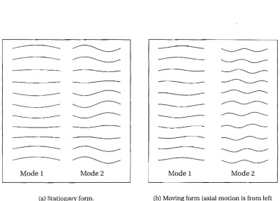
out of phase, each part being made up of combinations of either even (symmetric) or odd (asymmetric) eigenfunctions of the stationary problem. This (a) symmetry is a compelling reason to use these eigen-functions as the basis for the translating case. Once substituted into (2.17) the actual vibrations of the system are of nonconstant phase, and hence the waves propagate from one end of the string to the other, moving in the direction opposite to the trans-port speed (see Figure 2.3), Detailed discussion of this phenomena can be found in Wickert and Mote (1990) and Lengoc and McCallion (1996b,a).

The i'th exact free vibration frequencies for a moving string is given by (Lengoc and McCallion, 1996b)

27f

ae(a

+

c)(a c), (2.39)

where {J,

=J

R,,;~kI

is the material wave velocity and represents the critical speed at which all modes of vibration undergo divergent instability. Figure 2.4 plots the first

Table 2.1: Nominal parameters/or results o/Chapter 2.

f! b h E

(39)

2.3 RESULTS 21

---.

_~

----

_~

---

_---

----

~

-

- -

~

- -

----

~

---

-

---..

---

~

---

~

---

_---

---

~

- -

---

--- ---

- -

~

---

~

----

~

Model Mode 2 Mode 1 Mode 2

(a) Stationary form. (b) Moving form (axial motion is from left

to right).

Figure 2.3: Phase propagation in the first and second modes of vibration. Each set shows one

full cycle ofvibration.

i

k

....

!

~

'"" _~ ~

8

i'? i'?

5 5

~ _S.

'"

Jj _Jl

Translational speed, c lin s -1) TrrnlSlational speed, c [m s -1]

[image:39.595.86.486.105.392.2]

(a) Sinusoidal basis functions (b) Polynomial basis functions

(40)

four curves given by (2.39) and compares them against the approximate results pro-duced by the modelling of Section 2.1. Of note is the way that the sinusoids produce better approximations than the polynomials for a given number of basis functions, and that with higher numbers of basis functions the approximation accuracy is also improved.

'00

Translational speed, c 1m 5-1 J Translationalspee(l, c [ms-11

(a) Sinusoidal basis functions (b) Polynomial basis functions

Figure 2.5: Approximate frequency versus speed for a translating string,

The behaviour beyond the critical speed is plotted in Figure 2.5, where the ap-parent mode of instability is that of flutter, which is incorrect for an unloaded string. Increasing the number of basis functions serves to reduce the speed at which an apparent flutter instability occurs until the critical speed is reached, whereupon the mode of instability is again divergent. This points out the need to compare results for different numbers of functions to ensure that pointwise. convergence of the eigen-values has been achieved with respect to the number of basis functions used. Also, considering the practical application of this treatment and the limitation of the lin-ear theory at transport speeds nlin-ear or above the critical speed (Mote, 1966), it is unwise to use this modelling for high transport speeds.

2.3.2 Forced vibration

(41)

2.3 RESULTS 23

2.3.2.1 Distributed loads

The effect of increasing the spring force on a translating string, when no damping or follower loads are present (kd kf 0), is to increase monotonically all frequencies of vibration, as long as the transport speed is sub critical. The critical speed is not al-tered by the spring action in the case of the string; however, for the beam the critical speed is increased with increasing k_{s •}The eigenvalues remain purely imaginary as no damping has been introduced.

For ks kf 0 and kd

i-

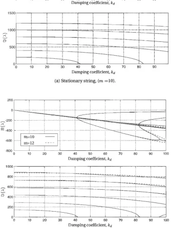
0 the eigenvalues contain nonzero real parts, the size of which depends on the amount of damping present. Figure 2.6 shows the change in frequency with increasing kd' for stationary and moving strings. The different ba-sis functions create different errors in the modal damping for the moving string at higher kd' with neither type producing superior performance. These errors may be reduced using more basis functions, but at the expense of computation and model size.

The follower force may be analysed by considering the x- and w-components separately, before considering their combined effect. Figure 2.7 shows a constant distributed follower load acting along the length of the string, and the corresponding lateral or w-component of that force.

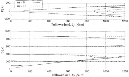
Figure 2.8 shows the effect of increasing lateral load upon the eigenvalues of the beam model. Here the tension has been reduced to zero to aid evaluation. The dot-ted line represents better accuracy in the Ritz approximation and shows the conver-gence in eigenvalues below follower loads of kf 700N/m in all of the four modes shown, (in fact values on the dotted line below kf

=

1000Nm-1 _{are convergent).}

The most interesting phenomenon in Figure 2.8 is the stiffening action of the lateral load upon the first mode of vibration, and the subsequent flutter instability around

k /' WON 1m. To verify this flutter instability Figure 2.9 plots typical modal forms for the first two modes at different values of k f. The two modes are obviously coalescing into one.

Figure 2.10 plots the variation in natural frequencies for a tensioned beam (R_o

=

150N) with increasing follower load. In this analysis t 1 (Table 2.1), and so the tension at:& fJ. remains at RD. This creates the destiffening seen in Figure 2.1O(b),

(42)

-400 ... + ... ~ ... ;. ... -.... -+ ... ····1··· .... ·::;:""'k:··· .! .•..•...•.. ;-. ..

c"" ...

··r···

! i

1500---,---r---r---r---r---~,_--~----_.----_,----~

500

P

-r-

i

- .

--r~---r--~-+--L..

OL---~----~----~----~----~----~--~~--~~--~~---o 10 20

Damping coefficient, kd (a) Stationary string, (m =10).

·600

10 20 30 60

Damping coefficient, kd

10 20 30 40 50 60 70 80 90 100

Damping coefficient, kd (b) Translating string. (c

=

20m/s).

[image:42.595.124.459.240.687.2]

(43)

2.3 HESUI.:rS 25

(a) Constant follower force.

[image:43.595.120.462.86.337.2] [image:43.595.78.498.449.699.2]

(b) Lateral component of follower force in (a), (kf ~~).

Figure 2.7: Distributed follower load and corresponding lateral component.

--,

""

'-.-'

c';?

200

rl

o

-200 o

1000

800

600

400

200

---m:::6 m=lO

t

-

I

i i _i

i _!

:

I

i

200 400 600 800

Follower load, k_flN/m]

200 400 600 800

Follower load, kf [N 1m]

- .1 ___ =

-~ ...

---+

----

-~

-

- - - -:

-=--1000 1200

1000 1200

(44)

kl = 0

1;:.1 100 i = = , ; r

-';:,1 125 --r--~=_-... - - - - _ _ r _

Figure 2.9: Modal forms of the first two modes of the stationary untensioned beam as lateral

follower load increases.

over polynomials as basis functions.

2.3.2.2 Point loads

Chen (1997) developed approximate solutions to the moving string under the point loadings described in this treatment, and Lengoc and McCallion (1999) provided an-alytical results. Figure 2.11 compares the anan-alytical results with this formulation. As expected the analytical results are lower than predicted using the approximate re-sults. Large numbers of basis functions are required to attain the analytical results as the very high spring stiffness (for which the results differ most) forces a discontin-uous slope in the modal forms at.'E Xd. !tis obvious that the basis functions used in this work cannot cope with such a restriction. However, such a high stiffness splits the string into two uncoupled spans (Lengoc, 1990), rendering the practical use of such a high stiffness useless.

Finally the effect of the follower point load acting on the moving string is shown in Figure 2.12. It is apparent that every mode except the third is markedly affected, with the critical speed being reduced to half that observed with no follower force. This is because the load is positioned half way along the length, at which point the slope of the deflection in odd-numbered modes is small, thereby creating a small lateral component.

2.3.3 Conclusion

(45)

2,3 RESULTS ₂₇

2000r---,---,---.---.---.---.~ Sinusoids

Polynomials

>

-o~----~----~----~~----~----~----~---~----~----~

o 500 1000 1500 2000 2500 3000 3500 4000 4500 5000

Follower load, kf [N/m)

(a) Lateral component of distributed follower force,

1000~---,---.·~~~----.---~~----,---~====~====~~~

o o

600

50

..

~--'::;,.'. ,

100 150 200 250 300 350

Followerload,kf [N/mJ

(b) In-line component of distributed follower force.

...;

,. '-....:

'-100 150 200 250 300 350

Follower load, kf [N/m]

(c) Full distributed follower load

Sinusoids Polynomials

400 450 500

Sinusoids Polynomials

""" ...

"

400 450 500

Figure 2.10: Effect of distributed follower load on vibration frequencies of the stationary

(46)

40

~ ~ 4~~===~'-+'---"-'----·-+C~---.. ---+--- ... ---.-.-~

g. ~

~ &

200/'-~~·=,="'::t~:::.··"··"···C'''''""" .. ~ ... ",, ,,·,1II\:b:···j ~ 200 _____ _

Tnmslational speed, c {rn s - 11

(a) Comparing spring action with points taken from Lcngoc and McCallion (1999).

0-J: ,

~~' ---~---~---~----~~.

Itallslatiollal speed, c 1m s -1 J

(b) Comparing damping action with points taken from Lengoc and McCallion (1999).

Figure 2.11: Effect of pointwise spring force and damping on vibration frequencies for the

moving string. Isolated points indicate data from Lengoc and McCallion (1999).

4 20

Translational speed. c [m s -1]

Figure 2.12: Effect of pointwise follower load on vibration frequencies for the moving string.

Isolated points indicate data from Lengoc and McCallion (1999). Xd

=

O.5f, kf

=

~Ro =

(47)

2.3 RESULTS 29

It has been shown that the gains of using the eigenfunctions of the stationary problem as basis functions are reduced when external loadings are applied, making the comparatively simple polynomials more attractive. However, use of the Gram-Schmidt process resulted in numerically unsound higher order polynomials, mean-ing that very large numbers of basis functions could not be accurately generated. Using a modified Gram-Schmidt procedure improved the situation to a degree.

(48)

(49)

Chapter 3 PLATES

This chapter considers current methods of describing axially moving plates that are influenced by in-plane tensions and edge loads, and proposes a new method which allows for more complex edge loading. The main application is high-strain wide bandsaws. The development of motion equations covered in the previous chapter is assumed, and therefore results follow directly from new formulations of relevant en-ergy expressions. The new method of describing edge loadings considers the cutting loads to act along a partial span of the blade, and also models the feed force during the cutting process. Also, the guides used on large bandsaws are modelled using two methods. Results for partial cutting system with guides is deferred until Chapter 5.

3.1 LITERATURE REVIEW AND BACKGROUND THEORY

Work on axially moving plates was started by Ulsoy and Mote (1982), by combining the kinetic energy due to translation with the bending and strain energies of plates. Defining the deflection surface to be w

=

w(x,

y,

t), and the plate to be

e

metres long,

b metres wide and h metres thick, the kinetic energy is

(3,1)

where c is the velocity of translation of the plate and is positive in the positive

:1;-direction, and p is the blade density. The strain energy due to bending is given by

(3.2)

where D = Eh3_/12(1

lJ2) is the plate rigidity. Ulsoy and Mote also considered the

(50)

create stresses throughout the blade, for which the resulting strain energy is

1

r

b

r

f

{(OW)2

ow ow

(OW)2}

Vs = 2

Jo Jo

N x ox

+

2Nxy ox oy

+

Ny oy dxdy, (3.3)

where Nx(x,y), Ny(x,y) and Nxy(x,y) are forces per unit length defining the pla-nar stress field throughout the plate. The conventions are that tensile stress is pos-itive and that pospos-itive shear elongates the diagonal joining the origin to the corner

(x, y)

=

(£, b). Both strain energy expressions are standard results for isotropic plates (see Timoshenko and Woinowsky-Krieger (1959) and Leissa (1969)). Ulsoy and Mote (1982) also compared experimental data from production scale bandmills with the theoretical results, but only for the transverse modes Of vibration.

A series of three papers (Lengoc and McCallion, 1995a,b,c), considered tangen-tial edge loading as a model of the cutting force, and assessed the blade stability in relation to parametric excitation of these loads. Furthermore, Lengoc and McCallion applied the idea of a follower force to the cutting edge, producing a nonconservative out of plane load as well as the tangential loading. The combined effects of bandmill strain, pretension and wheel tilting, translation speed and cutting loads were also considered in detail.

Lehmann and Hutton (1996) modelled the cutting loads on a more microscopic level, considering the cutting forces to act on each tooth. Also, the lumber density was assumed to vary analytically with proximity to a knot, and the gradient of the hardness function used to determine lateral loading on the blade. A full dynamic model of the band was presented, but not used because experimental cutting data was presented that showed the blade motion comprising primarily of frequencies below This led to the assumption of a "quasi-static" process, where the static blade stiffness rather than the blade dynamics influenced the sawn lumber surface. Therefore, the blade was assumed to be in static eqUilibrium, with the restitutive forces from the blade stiffness balancing the lateral cutting loads as well as forces from the interaction of the face of the blade with the sawn surfaces. Such a model will not account for the washboarding phenomenon, but is perhaps valid for low frequency effects such as snake and snipe. Lehmann and Hutton (1997) first uses the model of the previous work to establish the affect on tooth tip stiffness of parameters such as blade thickness, width, band strain etc. Then, the contact algorithm used in determining the side loads caused by the blade interaction with the sawn surfaces was shown to markedly affect the path of the blade near the idealised knot.

Active bandsaw control