Bayesian Non Parametric Mixture Model with Application to Modeling Biological Markers

(1)

ISSN Print: 2327-7211

DOI: 10.4236/jdaip.2019.74009 Sep. 16, 2019 141 Journal of Data Analysis and Information Processing

Bayesian Non-Parametric Mixture Model with

Application to Modeling Biological Markers

Mercy K. Peter

1

, Levi Mbugua

2

, Anthony Wanjoya

3

1_{Department of Mathematics, Pan African University Institute for Basic Sciences, Technology and Innovation, Nairobi, Kenya} 2_{Department of Statistics and Actuarial science, Technical University of Kenya, Nairobi, Kenya}

3_{Department of Statistics and Actuarial science, Jomo Kenyatta University of Agriculture and Technology, Nairobi, Kenya}

Abstract

The effect of treatment on patient’s outcome can easily be determined through the impact of the treatment on biological events. Observing the treatment for patients for a certain period of time can help in determining whether there is any change in the biomarker of the patient. It is important to study how the biomarker changes due to treatment and whether for different individuals located in separate centers can be clustered together since they might have different distributions. The study is motivated by a Bayesian non-parametric mixture model, which is more flexible when compared to the Bayesian Parametric models and is capable of borrowing information across different centers allowing them to be grouped together. To this end, this re-search modeled Biological markers taking into consideration the Surrogate markers. The study employed the nested Dirichlet process prior, which is eas-ily peaceable on different distributions for several centers, with centers from the same Dirichlet process component clustered automatically together. The study sampled from the posterior by use of Markov chain Monte carol algo-rithm. The model is illustrated using a simulation study to see how it per-forms on simulated data. Clearly, from the simulation study it was clear that, the model was capable of clustering data into different clusters.

Keywords

Bayesian Non-Parametric, Nested Dirichlet Process, Biomarker, Clustering, Surrogate Markers, Dirichlet Process, Markov Chain Monte Carlo

1. Introduction

To model hierarchical data when the distribution is not known is a big problem and has affected many researchers dealing with big data [1]. This is because of How to cite this paper: Peter, M.K.,

Mbugua, L. and Wanjoya, A. (2019) Baye-sian Non-Parametric Mixture Model with Application to Modeling Biological Markers. Journal of Data Analysis and Information Processing, 7, 141-152.

https://doi.org/10.4236/jdaip.2019.74009

Received: August 22, 2019 Accepted: September 13, 2019 Published: September 16, 2019

http://creativecommons.org/licenses/by/4.0/

(2)

DOI: 10.4236/jdaip.2019.74009 142 Journal of Data Analysis and Information Processing the disparity within the data, to account for the heterogeneity a Bayesian non-parametric model is necessary as it leads to flexible density estimates which are capable of identifying clusters of individuals with similar biomarker charac-teristics. Bayesian non-parametric mixture model is a good fit to model biologi-cal markers because it exhibits flexibility when modeling data which has a skewed and multi-modal distribution. The reason behind this is because data sets become bigger every day and require flexible models which can expand with the data. Mixture methods approach allows for probabilistic approach of clus-tering data points to different clusters [2]. The model also gives support to out of sample cluster assignments through computing the posterior probabilities for new data points.

In clinical trials, the importance of a treatment is either to decrease the burden of the disease for the patient or to eliminate the disease. To identify a biomarker which is changed by a treatment is not easy due to difficulties associated with the disease mechanisms. If a biomarker which is affected by the treatment has been identified, coming up with the association of the biomarker and the outcome is not easy because of the changes in the variability of the biomarker, patient re-sponse, and evaluation methods used. Thus, it is important to identify the changes each individual exhibit and whether there are changes or no changes as a result of the treatment [3]. The responses of individuals to treatment may be related, and identifying of groups of individuals sharing similar characteristics is of im-portant.

Many authors have applied the Bayesian non-parametric procedures to study various categories of biomarkers ranging from prognostic, predictive, phamaco-dynamic, and surrogate endpoints. For example, [4] studied the prognostic bio-markers and showed how they related to the clinical outcome using the Bayesian non-parametric procedures. Additionally, [3] studied the prognostic biomarkers using Bayesian parametric procedures, and finally [5] studied the surrogate end-points using the Bayesian methods. These studies identified the need to study biomarkers and determine how they are related with the clinical outcome.

Bayesian non-parametrics have a wide application in many areas especially big data analytics. Bayesian non-parametric methods are widely used to solve prob-lems where the size of the data changes leading to growth of the dimension of interest, for instance, in problems where the number of features varies with in-crease in the observed data. Also, they are commonly used in clustering and the number of clusters depends on the data being used. In general, in Bayesian non-parametrics models the number of parameters increases as the size of the data grows.

(3)

mea-DOI: 10.4236/jdaip.2019.74009 143 Journal of Data Analysis and Information Processing surement of the change, though, different distributions could give the same out-come.

Accordingly, [1] developed an integrative Bayesian predictive modeling frame-work to identify individual pathological brain states depending on the choice of fluoro-deoxyglucose positron emission tomography (PET) imaging Biomarkers and evaluated the relation of the states with a clinical outcome. The study would identify patient subgroup characterized by different biomarkers to produce the clinical outcome. The strategy also identified imaging Biomarkers with patho-logical states of the individuals and assumed that the latent individual state gets its values from one of the pathological states, and one of the states was a refer-ence point. The latent random variables were independent and identically dis-tributed taking a multinomial distribution. On the mixture weights a Dirichlet prior was used, considering a where the Gaussian distribution was considered, the mean was taken as one of the parameters to model the latent state specific random effect and to characterize the mean metabolic profile for individuals within the latent state. The Variance-covariance matrix captured the association between regions for individuals with latent state. A likelihood function was also established.

Additionally, [6] developed a Bayesian model to sample inference with availa-bility of inverse-probaavaila-bility weights. The study used a hierarchical method where the distribution of the weights from the non-sampled units was modeled and in-cluded predictors in a non-parametric Gaussian process. Simulation study was used to check how the procedure performed and compared to the classical de-sign-based estimator. The study concluded that Bayesian non-parametric finite population estimator is more appropriate compared with the classical estimator. Also, [7] compared the hierarchical Bayes model for biomarker subset effects in clinical trials to the profile likelihood method, to make references to the thre-shold parameter using bootstrap. The method provided improved sample prop-erties for probability coverage at 95% confidence interval.

Therefore, the importance of modeling surrogate markers in this study is to be able to determine the relationship between the baseline biomarker and the samples taken after an individual has been given some treatment. Bayesian non-parametric methods are flexible methods and will accurately indicate the relationship to show whether there is any change and be able to identify groups of individuals which have similar characteristics through clustering [8]. Also, the method is capable of showing whether after treatment the distribution of the biomarker changed through increase, decrease or it did not change at all.

(4)

DOI: 10.4236/jdaip.2019.74009 144 Journal of Data Analysis and Information Processing

2. General Modeling Framework

Let T denote the treatment effect, X represent the baseline biomarker, Y denote the post treatment values, and E the clinical outcome, and Z are the covariates which are present. If p(.) is a distribution, for instance, P E X Y Z T

(

| , , ,

)

, is a conditional distribution. If the treatment impact T is put into consideration, then the biomarker distribution will be affected. To address this then the inpatient change from X to Y is necessary. To assess the inpatient change, then putting into consideration of the relationship between X and Y because of the inpatient ef-fects is necessary. Due to the effect the treatment has on Y and the effect of the covariate to X or Y thus it leads to, P Y X Z T

(

| , ,

)

and P X Z

(

|

)

, though the distribution can either be highly disperse and complex. The model in this study will involve representation of a biomarker profile as ∆ = ∆

(

p X Y Z T

(

, | ,

)

_{, to}

symbolize the change made on the biomarker because of treatment, incorporat-ing them to the model to include the impact of the change on the outcome E. The model is also able to classify groups of individuals with various changes in Biomarker profiles depending on how the impacts of T and the change ∆ have on E. Thus, employing the probabilistic factorization then;

(

, , | ,

)

(

| , , ,

) (

, | ,

)

p E X Y Z T = p E X Y Z T p X Y Z T (1)

From Equation (1), the following assumptions are made;

1) p E X Y Z T

(

| , , ,

)

=p E

(

| , ,∆ Z T

)

, which implies, with the effect of the co-variates and the treatment, the impact of the (X, Y) on E is indicated by the change.

2) Also, the distribution of X and Y may be depended on the covariate, then the study assumes that both do not depend on the covariates.

A hierarchical Bayesian non-parametric model is employed for p X Y T

(

, |

)

and for the p E

(

| , ,∆ Z T

)

_{; a non-parametric regression model in the Bayesian}

case is employed, to give adaptable cluster estimates for individual’s specific dis-tributions of ∆ and their clusters. A hierarchical structure is obtained through making assumption of the individual’s specific Dirichlet processes being samples that are conditionally independent and obtained from a hyperprior which is also a Dirichlet process.

3. Proposed Model

Here the structure of the data is developed and the general model introduced. The subjects are indexed by

i

=

1, ,

_

N

_{. Assuming}_E_i_{is time-to-event outcome, let}

0 i

E be the observed time of the event with ε =i 1, if Ei0 =Ei, and 0 if Ei0<Ei.

For 0

(

0 0

)

1, , N

E = E _ E _, ε =

(

ε₁, , εN

)

, and Zi =

(

Z Z1i, 2i, , Zki

)

be the

base-line covariates with Z =

(

Z Z1, , ,2  ZN

)

. For the ith individual let ni and mi be

the measurement frequencies of the levels of the biomarker obtained before treatment and after. Let Xi=

(

Xi1, , Xini

)

and Yi =

(

Yi1, ,Yimi

)

be the

indi-viduals pre and post-treatment biomarker values, where, X =

(

X X1, 2, , XN

)

and Y =

(

Y Y1, , ,2 YN

)

.

(5)

DOI: 10.4236/jdaip.2019.74009 145 Journal of Data Analysis and Information Processing change for the levels of the biomarker before and after treatment. Where Ti is the

treatment given to the ith_{individual and ∆ is some measure of distributional}

dis-tance. The distributional distance is defined on a sample space cumulative den-sity function (Cdf) of one-dimensional random variables, which is the distribu-tional distance between the two cdf’s FX and FY in the space of cumulative

densi-ty function. The vertical quantile function is;

( )

(

1

( )

)

( )

, for 0,1

X Y Y X

Q p ₌F F− p p_∈ ₍₂₎

where, Equation (2) is a quantile function of order p which is a representation of the functional for the density plot. The quantile function allows for comparison of various functions for all the distributions. For instance, QX Y,

( )

p =0.5 is

used in median tests. Also, the vertical quantile function is associated with the Receiver Operating Characteristic (ROC) curve represented as

( )

1

(

)

ROC p = −1 F FY X− 1−p ,

where FX and FY are the cdf’s of the diagnostic variables in the populations. Here,

the interest is not to assess the diagnostic performance for a biomarker; however, to evaluate the targeted treatment, the vertical quantile function is estimated by taking into consideration the distribution functions FXi and FYi for the subject

levels of biomarker for different individuals. Therefore, the distributional change is;

( )

(

( )

)

(

)

1 ,

0QX Y p p EF F Yd Y X p X Y

∆ =

_∫

= = < (3)

Equation (3) corresponds to the area under the curve which is majorly applied in diagnostic studies. Thus, ∆ represents the change of the distribution of the biomarkers for the ith_{individual, because of the treatment administered to the}

subject. A posterior estimate with p X

(

ij <Yik| data

)

>0.5, means that the

indi-vidual’s distribution has moved to the right, that is, there is a biomarker increase. Also, p X

(

ij <Yik| data

)

<0.5, shows a change to the left side, hence a decrease

in the biomarker levels, and p X

(

ij <Yik| data

)

≈0.5, indicates no remarkable

change. Thus, from Equation (1) the patient level data likelihood is;

(

0_, _, _{, |} _, _{, ,}

) (

0_{, |} _{, ,}

)

(

_{, | ,}

)

i i i i i i i i i i i i i

p T ε X Y Z T β θ = p T ε ∆ T β p X Y T θ ₍₄₎

For β a vector of parameters for regression modeling and θ parameterizes the hierarchical model.

(

0_{, | , , , ,}

) (

0_{, | , , ,}

)

p T ε X Y Z T β = p T ε ∆ Z T β ₍₅₎

Thus, T0_{, follows one of the common distribution like the log-normal, where}

(6)

measure-DOI: 10.4236/jdaip.2019.74009 146 Journal of Data Analysis and Information Processing ments of the biomarker are samples are obtained from unknown individuals distributions with i1, , in ~

in i

d Xi

X  X F and i1, , im ~ in i

d Yi

Y Y F , Where Xi and Yi are

vectors of subject specific measurements. FXi and FYi are modeled separately

us-ing mixtures of Gaussian distribution denoted by mean µ and standard deviation δ, that is N

(

µ δ,

)

_{. The pdf and cdf are denoted by} φ µ δ

(

., ,

)

_and Φ

(

t, ,µδ

)

_.

The mixture components are defined as wi for each component with the

con-straint such that, 1 1 k

i i= w =

∑

, implying that the total probability distribution will normalize to 1. Thus, the Gaussian mixture model is represented as;

( )

k₁

(

| ,

)

i i i

i

p x =

∑

₌ w N x µ δ ₍₆₎

(

| ,

)

1 exp

(

₂

)

2

2 2 i i i i i x

N x µ δ µ

δ δ −    =  − 

π _

Assuming a DP with a concentration parameter α and a base distribution G0.

Then, for each individual

i

=

1, ,



N

it follows that;

(

)

| , ind~ , , 1, ,

ik Yik Yik Yik Yik i

Y µ δ N µ δ k=  m

(

)

1

| , ind~ , , 1, ,

ij Xij Xij Xi

p

j Xij i

j

X µ δ

∏

₌ N µ δ j= _ n ₍₇₎

(

0

)

, , , | iid~ , ~ DP ,

Yik Yik Xij Xij G G G G

µ δ µ δ α

where, α =1, and G0 =N

(

µ δ,

)

.

Let θXij =

(

µ δXij, Xij

)

and θYij =

(

µ δYij, Yij

)

. Under the mixture model

θ

Xij and

θ

Yij are sampled from some mixing distributions GXiand GYi as follows;

1 1 , , | , , | ~ ~ ind

Xi Xini Xi Xi

ind

Yi Yimi Yi Yi

G G

θ θ



 (8)

This means that the conditionals on the realizations of GXiand GYi, thus, the

dis-tributions for the Xi and Yiare the following mixtures;

(

)

(

) (

)

(

)

(

) (

)

1

| ; d

ni

X i Xi j ij Xij Xi Xij

mi

Y i Yi j ik Yik Yi YiK

f x G x G

f y G y G

φ

θ

φ

θ

= = = =

∏

∫

∏

∫

(9)

To assess the change in the distribution of Yi verses Xi in terms of ∆i so as

to be able to investigate the association of the change with the outcome and clas-sify groups of subjects which have the same biological responses. Additionally, a prior model is defined on GXi and GYi and it involves the Dirichlet process (DP),

which is commonly preferred prior probability model due to its clustering capa-bility. [9] expressed this as G~ DP ,

(

α G0

)

, which is a random distribution G

following a DP that has a base distribution E G

( )

=G0 and a concentration

parameter α _. α_{Shows significant properties, that is, how}_G_{varies about the} mean (base distribution), where a smaller value of α shows high uncertainty and vice versa.

Since G are discrete samples, they have some positive probability ties, as some

Yij

(7)

esti-DOI: 10.4236/jdaip.2019.74009 147 Journal of Data Analysis and Information Processing mate GXi and GYi for each subject, though it lacks the clustering properties of the

distributions for all individuals or among the pre and post treatment values ob-tained. Clustering is necessary so as to identify the change after the treatment for all the individuals. Thus, the change is obtained by assuming that GXi and GYi are

realizations of a common Dirichlet process mixture model (DPMM). In a DPMM the individual’s realizations of GXi and GYi are shared across and for each

sub-ject’s pre and post treatment values. Therefore, GXi and GYi are independent

conditional samples from the same the Dirichlet process, then;

1 1

~ _ok and ~ _ok

Xi k k G Yi k k G

G ∞ π δ G ∞ π δ

= =

∑

(10)

where G0k is a realization from a common DP prior that is DP ,G

(

γ 0*

)

which

has a base distribution * 0

G and a concentration parameter γ_{, then;}

( )

* *

( )

1

. _pok .

ok p pok

G w δθ

∞ =

=

∑

₍₁₁₎

Here * *

0

~

pok G

θ

. Therefore each GXi and GYi is automatically obtained from a

collection of different distributions that is the G0k’s.

4. Formulation of the Hierarchical Model

The hierarchical model is formulated using the nested Dirichlet Process (nDP) which is as follows;

(

)

(

*

)

0

, ~ DP , ,

Xi Yi

G G α γ G ₍₁₂₎

In the earlier discussions, it is clearly expressed that ∆i_{is a functional of}

(

_i, | ,_i _i _i

)

p X Y Z T , which in the nDP is determined by the realizations GXi and GYi

in Equation (10). Since the Dirichlet process given by Equation (10) has a dis-crete support and πk’s in the equation cannot be neglected, then it shows a non-trivial probability where GXi =GYi, which means that the treatment has no biological impact on patient i, this is clearly shown through the posterior esti-mate of the ∆i _{. Additionally, there is also non-trivial probability that}

(

G GXi, Yi

) (

= G GXi, Yi

)

for i i≠ ′ which implies ∆ = ∆i i′, implying the

bio-markers profiles for individuals i and i' are in one cluster. To complete the model the base distribution *

0

G is specified and it is defined as a Normal-Inverse Gamma (N-IG) distribution for the mean and precision pa-rameters in the Normal model and α and γ_{are assigned independent Gamma} priors, thus, the hierarchical probabilistic model.

4.1. Biomarker Profiles Likelihood

The Biomarker Profiles Likelihood is as below;

(

)

| , ind~ , , 1, ,

ik Yik Yik Yik Yik i

Y µ δ N µ δ k=  m

(

)

~ 1

| , ind p , , 1, ,

ij Xij Xij j Xij Xij i

X µ δ

∏

₌ N µ δ j=  n (13)

( )

(

)

(

)

i E G YYi ik p Xij Yik

(8)

4.2. The Model and the Priors

(

,

)

E and

(

,

)

E

Xij Xij Xij Yik Yik Yik

θ = µ δ θ = µ δ

| ~ and | ~

Xij GXi GXi YiK GYi GYi

θ

(

)

(

*

)

0

, ~ nDP , ,

Xi Xi

G G α γ G ₍₁₄₎

(

)

(

)

~ Gam a bα, α , ~ Gam a bγ, γ

α γ

(

)

*

0~ N-IG 0, , ,0 0 0

G

µ

k a d

(

β δ, E

)

~ N-IG

(

µ1, , ,k a d1 1 1

)

where, the fixed hyper parameters are; μ0, k0, a0, d0, μ1, k1, a1, d1.

5. Posterior Computation

To compute the joint posterior distribution for model parameters, this is done computationally. Thus Markov Chain Monte Carlo (MCMC) algorithm for posterior inference is used. The full conditional to update the nDP are gotten using the method described by [10] depending on a truncated Dirichlet process. At each iteration, for the baseline distribution *

0

G , parameters are continuously updated based on all the samples represented by the biomarker values. The algo-rithm is developed using a truncation of a Dirichlet process to give approximate truncation to the stick breaking process of a Dirichlet process leading to method of computation in finite mixture models.

This assumes that, individuals are clustered into K groups and for every indi-vidual the observations on the biomarker level can be clustered into L groups. To provide support for the estimation of both clinical and biological effects together, the proposed model accounts completely for the uncertainty of the random quantities, together with variability of the ∆i’s to express the variation of the population. In every iteration the Gibbs sampling algorithm gives samples of the distribution of the biomarker (GXi, GYi) for every individual, used to get the

bio-marker profile ∆i. This can be easily illustrated by Considering the model as in Equation (13) and Equation (14), to obtain samples from the posterior after the burn in, every value that is sampled ( *

i

∆ ) is obtained by getting the average for the estimates of the posterior

(

*_, *

)

Xi Yi

G G of the subjects distributions of biomark-ers. From Equation (9) and Equation (10), it is clear that every mixing distribution G0k, F t G

(

| 0k

)

( )

t;

θ

G d0k

( )

θ

i1wlr*

( )

t;

θ

lr*

∞ =

= Φ =

∑

Φ for F G= Xi or GYi, to

obtain the biomarker profile for the posterior then, Equation (15) is applicable;

( )

(

)

( )

* * * * *

i =EG G YYi Xi ik G y dG y dyXi Yi

∆ =

_∫

₍₁₅₎

where * * *

1 l

Xi l l

G w

δ

θ

∞ =

=

∑

_and * * *

1 l

Yi l l

G w

δ

θ′

∞ ′ =

=

∑

_{thus the estimate of the} post-erior biomarker profile is obtained by dividing the mean with the postpost-erior val-ues which is;

* *

* * *

2* 2*

1 l l

l l l l l

l l

w w µ µ

δ δ ′ ′ ′ ′   ₋    

∆ = − Φ

 _ ₊ _

 

(9)

6. Simulation Study

In this section, a simulation study is presented to show the capability as well the ability of the nested Dirichlet Process when modeling biological markers to give accurate density estimates by obtaining strength from different centers. In the simulation, N samples are obtained from a mixture of four Gaussian distribu-tion.

( )

k

( )

i k i

f x =

∑

w f x ₍₁₇₎

Equation (17), is a representation of a mixture of Gaussian distribution with wi

mixing weight for every component, and f xk

( )

is the component which can

be represented by any distribution. Here, the components are represented by a normal distribution such that the mixture distribution becomes;

( )

k

(

_, 2

)

i i i

i

f x =

∑

w N

µ δ

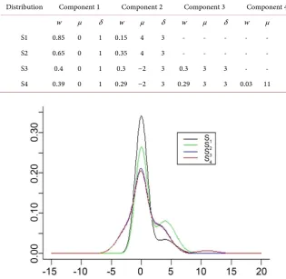
₍₁₈₎

The study generates J = 40 samples each of size 100, for j=1, ,40 . Every sample is obtained from a mixture of k = 4 Gaussian mixtures summarized in Table 1, and plotted in Figure 1.

The true distributions are plotted in Figure 1.

[image:9.595.209.525.403.710.2]

Distribution S1 and S2 are asymmetric with a mixture of two Gaussian com-ponents with different weights. For distribution S3 and S4, they share three

Table 1. The components of various Gaussian distributions.

Distribution Component 1 Component 2 Component 3 Component 4 w μ δ w μ δ w μ δ w μ δ S1 0.85 0 1 0.15 4 3 - - - - S2 0.65 0 1 0.35 4 3 - - - - S3 0.4 0 1 0.3 −2 3 0.3 3 3 - - - S4 0.39 0 1 0.29 −2 3 0.29 3 3 0.03 11 3

(10)

DOI: 10.4236/jdaip.2019.74009 150 Journal of Data Analysis and Information Processing mixture components which are located at the origin, with difference only on the fourth component of the distribution S4.

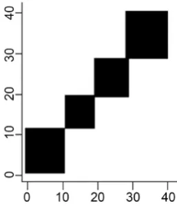
The true cluster memberships are plotted in Figure 2. It represents the true cluster membership si for J = 40 samples through plotting I (si = sj) for all the

pairs. The samples are ordered by their true clusters. Therefore, these are simu-lation conditions with well separated true distributional clusters.

The same number of samples has been simulated for the each of the four true distributions. To obtain the posterior simulation, then; the precision parameters α and γ are both fixed to 1 and the Normal-Inverse Gamma distribution which is the baseline measure (base distribution) are µ =0 0, λ =0.01, a=3,

and

b

=

1

_{, such that; NIG(0, 0.01, 3, 1). Therefore, a priori}_E

(

_{µ δ}_| 2

)

₌₀_,

(

_| 2

)

₁₀₀ 2

V µ δ = δ _, _E

( )

_δ2 ₌₁_{, and} _V

( )

_δ2 ₌₃_.

The algorithm described in Section 5 is used to obtain the samples of the posterior distribution using the nested Dirichlet Process. The study runs MCMC chain with 12,000 iterations, discarding the first 2000 iterations and thinning out to save one in every 10 iterations.

The estimated distributions E F y

(

k|

)

for each distributional cluster are

represented in Figure 3. Figure 3 is an image of Figure 1. This is a clear indica-tion that the prior and the posterior samples obtained after the MCMC draws are the same and reflect the distribution where each of the observation has been obtained from. The posterior draws are drawn from all the distributions with all the components. Hence, the posterior and the prior distribution are the same. Thus, in this case when using the Bayesian non-parametric mixture model it re-flects the individual biomarker distributions before treatment taking the same form as the after treatment measurements drawn from different centers.

Also, the posterior cluster memberships takes the same form as the true clus-ter memberships as clearly shown in Figure 4.

[image:10.595.307.436.557.707.2]

The posterior co-clustering probabilities take the same form as the true cluster membership. The model developed is able to classify groups of individuals from different centers (distributions) to one group. The individuals are placed into the groups as per the prior information which is available. Hence, the diagram dis-plays four clusters similar to the estimated distribution as shown in Figure 4.

(11)

[image:11.595.249.496.72.247.2]

Figure 3. Representation of the estimated distribution.

Figure 4. Representation of the posterior co-clustering probabilities for all the

distribu-tions.

7. Conclusions

We introduced a model using the truncated nested Dirichlet process to identify groups of individuals who respond similarly to the same treatment for a speci-fied biological marker. An MCMC algorithm has been used to estimate the posterior inference. Since the nDP is a non-parametric model, it has the capabil-ity of grouping all the observations from the mixture depending on the entire distribution, rather than selecting particular features of the distribution. In the simulation study the proposed method for biological markers showed a good performance in differentiating the unimodal distributions from the multimodal distributions.

[image:11.595.306.441.279.438.2]

(12)

DOI: 10.4236/jdaip.2019.74009 152 Journal of Data Analysis and Information Processing longitudinal biomarker values to account for individuals biomarker processes. This work can be extended to model the relationship between two or more groups of data after the individuals have been clustered. Also, the procedure did not take into consideration of the covariates which might affect the biomarkers. This can also be incorporated so as to see whether they have any effect.

Acknowledgements

We thank the Editor and the referee for their comments. Our research is funded by the African Union, this support is greatly appreciated.

Conflicts of Interest

The authors declare no conflicts of interest.

References

[1] Chiang, S., Guindani, M., Yeh, H.J., Dewar, S., Haneef, Z., Stern, J.M. and Vannuc-ci, M. (2017) A Hierarchical Bayesian Model for the Identification of Pet Markers Associated to the Prediction of Surgical Outcome after Anterior Temporal Lobe Resection. Frontiers in Neuroscience, 11, 669.

https://doi.org/10.3389/fnins.2017.00669

[2] Orbanz, P. and Teh, Y.W. (2011) Bayesian Nonparametric Models. Springer, Berlin, 81-89.https://doi.org/10.1007/978-0-387-30164-8_66

[3] Morita, S., Thall, P.F., Bekele, B.N. and Mathew, P. (2010) A Bayesian Hierarchical Mixture Model for Platelet-Derived Growth Factor Receptor Phosphorylation to Improve Estimation of Progression-Free Survival in Prostate Cancer. Journal of the Royal Statistical Society: Series C (AppliedStatistics), 59, 19-34.

https://doi.org/10.1111/j.1467-9876.2009.00680.x

[4] Graziani, R., Guindani, M. and Thall, P.F. (2015) Bayesian Nonparametric estima-tion of Targeted Agent Effects on Biomarker Change to Predict Clinical Outcome. Biometrics, 71, 188-197.https://doi.org/10.1111/biom.12250

[5] Cowles, M. (2004) Evaluating Surrogate Endpoints for Clinical Trials: A Bayesian Approach. Technique Report, University of Iowa, Iowa City, IA.

[6] Si, Y., Pillai, N.S. and Gelman, A. (2015) Bayesian Nonparametric Weighted Sam-pling Inference. Bayesian Analysis, 10, 605-625.

https://doi.org/10.1214/14-BA924

[7] Chen, B.E., Jiang, W. and Tu, D. (2014) A Hierarchical Bayes Model for Biomarker Subset Effects in Clinical Trials. Computational Statistics and Data Analysis, 71, 324-334.https://doi.org/10.1016/j.csda.2013.05.015

[8] Kai, C. and Wenshan, C. (2012) Spike-and-Slab Dirichlet Process Mixture Models. Open Journal of Statistics, 2, 512-518.https://doi.org/10.4236/ojs.2012.25066

[9] Ferguson, T.S. (1973) A Bayesian Analysis of Some Nonparametric Problems. The Annals of Statistics, 1, 209-230.https://doi.org/10.1214/aos/1176342360

[10] Rodriguez, A., Dunson, D.B. and Gelfand, A.E. (2008) The Nested Dirichlet Process. Journal of the American Statistical Association, 103, 1131-1154.