A non parametric maximum test for the Behrens–Fisher problem

A nonparametric maximum test for the Behrens-Fisher problem

Anke Welz1_{, Graeme D. Ruxton}2_{, Markus Neuhäuser}1

1. Department of Mathematics and Technology, RheinAhrCampus, Koblenz University of Applied Sciences, Joseph-Rovan-Allee 2, 53424 Remagen, Germany

2. School of Biology, University of St Andrews, St Andrews, Fife KY16 9TH, UK

Abstract: Non-normality and heteroscedasticity are common in applications. For the

comparison of two samples in the nonparametric Behrens-Fisher problem, different tests have been proposed, but no single test can be recommended for all situations. Here, we propose combining two tests, the Welch t test based on ranks and the Brunner-Munzel test, within a maximum test. Simulation studies indicate that this maximum test, performed as a

permutation test, controls the type I error rate and stabilizes the power. That is, it has good power characteristics for a variety of distributions, and also for unbalanced sample sizes. Compared to the single tests, the maximum test shows acceptable type I error control.

Key words: Behrens-Fisher problem; Brunner-Munzel test; maximum test; Welch t test

1. Introduction

be superior to traditional tests, but “no one robust method is ideal for all situations” (Grissom, 2000). Fagerland and Sandvik (2009a, 2009b) investigated several tests for skewed

distributions and unequal variances, they also conclude that no single test can be

recommended for all scenarios. Furthermore, transformations to overcome the heterogeneity of variances are also problematic (Grissom, 2000), in particular when samples are small (Neuhäuser, 2010).

When no test is ideal for all situation, one can try to combine different tests. Recently, Neuhäuser (2015) combined the t test and Wilcoxon’s rank-sum test in a maximum test. This maximum test controls the type I error rate and is a more powerful strategy than always selecting one of the single tests. The principle of using the maximum of several competing test statistics as a new statistic, combined with using the permutation distribution of the maximum for inference, is common in areas such as statistical genetics (Neuhäuser and Hothorn, 2006).

Here, we apply the idea of a maximum test to the non-parametric Behrens-Fisher problem. In the nonparametric Behrens-Fisher problem, one does not test the general alternative of any difference between the distribution functions of the two groups. Instead, one tests whether there is a tendency towards smaller, or larger, values in one group. An

appropriate null hypothesis is 𝐻0𝐵𝐹: 𝑝 = 0.5 , with p being the relative effect defined as

p = P(Xi < Yj) + 0.5 P(Xi = Yj), where Xi and Yj are observations in group 1 and 2, respectively. The random variable 𝑋 tend to take smaller values than the random variable 𝑌 if 𝑝 > 0.5; 𝑋 tends to take larger values than 𝑌, if 𝑝 < 0.5; stochastic equality holds if 𝑝 = 0.5

(Neuhäuser, 2012; Brunner and Munzel, 2013).

is equivalent to the equality of expected values of rank scores (Vargha and Delaney, 1998). However, it should be noted that these t tests have a heuristic justification only, their appropriateness and robustness for the nonparametric Behrens-Fisher problem is based on empirical studies only (Delaney and Vargha, 2002). In general, the rank transformation is not valid in the Behrens-Fisher problem (Brunner and Munzel, 2013). Indeed, even the rank Welch t test can become liberal (i.e. taking a true type I error rate greater than the nominal level) when the variance difference between the groups is large, and for discrete distributions when sample sizes are small. However, Cribbie et al. (2007) demonstrated in a simulation study that both the Brunner-Munzel test and the Welch t test based on ranks control the type I error rate for a wide range of situations. With regard to power, the Welch t test was superior to the Brunner-Munzel test across the situations explored.

In this article, we investigate several tests, including some maximum tests, in a simulation study, and apply the proposed test to an example data set.

2. Methods

We compare two independent random samples 𝑋1, … , 𝑋𝑛 and 𝑌1, … , 𝑌𝑚, where 𝑋𝑘 ∼ 𝐹1 i.i.d., 𝑘 = 1, . . , 𝑛, and 𝑌𝑖 ∼ 𝐹2 i.i.d. , 𝑖 = 1, … , 𝑚, 𝑁 = 𝑛 + 𝑚. The distribution functions 𝐹1 and 𝐹₂ are arbitrary distributions, but one-point distributions are excluded. We perform two-sided tests for the non-parametric Behrens-Fisher problem, i.e.

𝐻₀𝐵𝐹_{: 𝑝 = 0.5 versus 𝐻}

1𝐵𝐹: 𝑝 ≠ 0.5.

In the case of symmetric distributions with finite expected values, testing stochastic equality is equivalent to the test of equality of expected values. Therefore the classical parametric Behrens-Fisher problem is a special case of the non-parametric Behrens-Fisher problem (Neuhäuser, 2012).

statistic is based on ranks too; for min(n, m) ≥ 10 its null distribution can be approximated by a t distribution (Brunner and Munzel, 2000).

As a new test we combine two of the three above-mentioned test statistics. In order to make the statistics comparable, they are standardized by dividing each statistic 𝑡_𝑖 by its standard deviation 𝑠𝑑𝑖. Since the statistics used are approximately t distributed, the standard

deviation 𝑠𝑑_𝑖 is approximated by the corresponding degrees of freedom, i.e. 𝑠𝑑 = √_𝑑𝑓−2𝑑𝑓 .

Because we consider the two-sided test, the absolute values of the standardized test statistics are used to construct the maximum test statistic as follows:

𝑡𝑀𝐴𝑋 = max ( | 𝑡1 𝑠𝑑1| , |

𝑡2 𝑠𝑑2|)

with 𝑡₁ and 𝑡₂ one of the above-mentioned test statistics 𝑡_{𝑟𝑎𝑛𝑘}, 𝑡_{𝑊𝑟𝑎𝑛𝑘} or 𝑡_𝐵𝑀.

The single tests as well as the maximum tests are performed as permutation tests, i.e. the inference is based on the permutation null distribution of the test statistic (see e.g. Berry et al., 2016). Thus, the tests can also be used in the presence of ties as well as for small samples. The p-value of the permutation test is the proportion of permutations where the corresponding absolute value of the respective test statistic is higher than or equal to the absolute value of the statistic computed for the original data. The permutation test can be based on all possible

permutations, in total (𝑁_𝑛) permutations, or as an approximate permutation test based on a

simple random sample of permutations.

test with the Brunner-Munzel statistic. We also use this approach of Neubert and Brunner (2007) including the way they compute the variance of the Brunner-Munzel statistic.

Note that, by choosing 𝑡_{𝑟𝑎𝑛𝑘} as the test statistic, the Wilcoxon rank-sum test is applied indirectly, because 𝑡_{𝑟𝑎𝑛𝑘} is a monotone function of the Wilcoxon rank-sum statistic (Conover and Iman, 1981).

In order to evaluate differences between the actual type I error rates and the nominal significance level α, Bradley’s (1978) liberal criterion is used. According to this criterion for robustness, applied by other recent investigations such as Haidous and Sawilowsky (2013) and Nguyen et al. (2016), an actual rate between 0.5α and 1.5α is deemed acceptable.

3. Simulation Study

In a simulation study performed with R (using the libraries stats and lawstat), we evaluate the maximum tests as well as the single tests. All tests were carried out as permutation tests. As mentioned above, in the non-parametric Behrens-Fisher problem we cannot conclude that a permutation test guarantees the nominal significance level. Therefore, it is important to investigate the actual type I error as well as the power of the investigated tests.

We consider different distributions, including the distributions discussed by Neubert and Brunner (2007). The distributions are:

(i) Two normal distributions 𝑋 ∼ 𝑁(0,1) and 𝑌 ∼ 𝑁(𝑠ℎ𝑖𝑓𝑡, 𝜎_𝑌2₎

(ii) Two uniform distributions 𝑋 ∼ 𝑈[0,1] and 𝑌 ∼ 𝑈[𝑠ℎ𝑖𝑓𝑡, 𝑠ℎ𝑖𝑓𝑡 + 𝜎𝑌 ]

(iii) Two Poisson distributions 𝑋 ∼ 𝑃𝑜𝑖𝑠(𝜆 = 5) and 𝑌 ∼ 𝜎_𝑌 ∙ 𝑃𝑜𝑖𝑠(𝜆 = 5) + 𝑠ℎ𝑖𝑓𝑡

(iv) Two log-normal distributions 𝑋 ∼ 𝑙𝑜𝑔𝑁𝑜𝑟𝑚(𝜇 = 0, 𝜎2 _{= 1) − 1 and}

𝑌 ∼ 𝜎_𝑌 ∙ (𝑙𝑜𝑔𝑁𝑜𝑟𝑚(𝜇 = 0, 𝜎2 _{= 1) − 1 − 𝑠ℎ𝑖𝑓𝑡)}

𝑌 ∼ 𝜎_𝑌 ∙ (𝐸𝑥𝑝(𝜆 = 2) −ln(2)₂ − 𝑠ℎ𝑖𝑓𝑡)

By choosing the values 1, √2, and 2 for the parameter 𝜎_𝑌 , we realize the variance ratios (VR)

1:1, 1:2 and 1:4. The distributions in situations (iv) and (v) are shifted by 1 or ln(2)₂ ,

respectively, in order that their medians are 0, thus for 𝑠ℎ𝑖𝑓𝑡 = 0 the medians of both groups are equal.

The distributions discussed in Neubert and Brunner (2007) are a normal distribution

against one 𝜒2 _{distribution and two bimodal distributions:}

(vi) A normal distribution 𝑋 ∼ 𝑁(𝜇 = 2.5745, 𝜎2 _{= 2) against a 𝜒}2 _distribution

𝑌 ∼ 𝜒_𝑑𝑓=32 _{+ 𝑠ℎ𝑖𝑓𝑡}

(vii) Two bimodal distributions 𝑋 ∼ 0.7 ∙ 𝑁(𝜇 = 4, 𝜎2 _{= 1) + 0.3 ∙ 𝑁(𝜇 = 8, 𝜎}2 _{= 1) and}

𝑌 ∼ 0.3 ∙ 𝑁(𝜇 = 2.07 + 𝑠ℎ𝑖𝑓𝑡, 𝜎2 _{= 2) + 0.7 ∙ 𝑁(𝜇 = 3 ∙ (2.07 + 𝑠ℎ𝑖𝑓𝑡), 𝜎}2 _{= 2)}

The VR in (vi) is 1:3 and the VR in (vii) is 1:2. By setting 𝑠ℎ𝑖𝑓𝑡 = 0 in (vi) and (vii) the relative effect 𝑝 is equal to 0.5.

Simulations were performed for balanced and unbalanced sample sizes with (𝑛, 𝑚) = (10,10), (10,20), and (20,10), combined with the different variance ratios mentioned above.

For each configuration, 10,000 simulation runs were performed, in each run 1,000 permutations were chosen to compute p-values.

and BM has a type I error rate much closer to α. Therefore, we propose the maximum test with Welch t statistic on ranks and the Brunner-Munzel statistic. As the displayed results indicate, this maximum test has a type I error rate relatively close to the nominal level 5%, often closer to 5% than the single tests, in particular when the smaller sample has the higher variance, a situation where all the single tests are liberal. Further results for this maximum test using Wrank and BM are presented below.

Fig. 1 and 2 about here

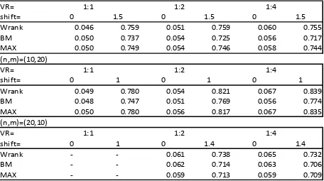
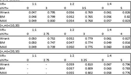
Tables 1 to 3 show the simulated type I error rates and the power of the proposed maximum test with Welch t statistic on ranks and the Brunner-Munzel statistic (abbreviated by MAX) and the single tests used to construct this maximum, for different distributions (log-normal, exponential, and Poisson). Again, the tests are robust according to Bradley’s criterion, the maximum test's control of the type I error rate seems acceptable and is usually better than that of the single tests. The results for the distributions (vi) and (vii) are similar, see Table 4.

For all investigated distributions the maximum test stabilizes the power; the power of the maximum is always between the powers of the single tests, often the maximum test has a power similar to that of the more powerful of the two single tests.

Above, the nominal significance level 5% was used. However, we also investigated the nominal levels 1%, 2.5% and 10%. In these cases, the results are analogous, see

more clearly and a few times more often. However, there are also scenarios where one of the single tests has a type I error closer to α than the maximum test, in particular for α = 10%.

Table 1. Simulated type I error rates and power in the case of the log-normal distribution (α=5%)

(n,m)=(10,10)

VR= 1:1 1:2 1:4

shift= 0 1.5 0 1.5 0 1.5

Wrank 0.046 0.759 0.051 0.759 0.060 0.755

BM 0.050 0.737 0.054 0.725 0.056 0.717

MAX 0.050 0.749 0.054 0.746 0.058 0.744

(n,m)=(10,20)

VR= 1:1 1:2 1:4

shift= 0 1 0 1 0 1

Wrank 0.049 0.780 0.054 0.821 0.067 0.839

BM 0.048 0.747 0.051 0.769 0.056 0.774

MAX 0.050 0.780 0.056 0.817 0.067 0.835

(n,m)=(20,10)

VR= 1:1 1:2 1:4

shift= 0 1 0 1.4 0 1.4

Wrank - - 0.061 0.738 0.065 0.732

BM - - 0.062 0.714 0.063 0.706

MAX - - 0.059 0.713 0.059 0.709

(n,m)=(10,10)

VR= 1:1 1:2 1:4

shift= 0 0.55 0 0.5 0 0.55

Wrank 0.049 0.772 0.050 0.742 0.060 0.788

BM 0.051 0.760 0.053 0.717 0.058 0.754

MAX 0.052 0.767 0.054 0.729 0.060 0.777

(n,m)=(10,20)

VR= 1:1 1:2 1:4

shift= 0 0.4 0 0.4 0 0.35

Wrank 0.049 0.816 0.054 0.864 0.066 0.811

BM 0.048 0.792 0.050 0.826 0.054 0.75

MAX 0.049 0.815 0.054 0.862 0.065 0.808

(n,m)=(20,10)

VR= 1:1 1:2 1:4

shift= 0 0.4 0 0.6 0 0.5

Wrank - - 0.056 0.857 0.065 0.755

BM - - 0.057 0.840 0.063 0.729

Table 3. Simulated type I error rates and power in the case of the Poisson distribution (α=5%)

(n,m)=(10,10)

VR= 1:1 1:2 1:4

shift= 0 3 0 3.5 0 5

Wrank 0.047 0.795 0.056 0.769 0.061 0.826

BM 0.048 0.799 0.052 0.765 0.056 0.82

MAX 0.049 0.800 0.054 0.768 0.057 0.823

(n,m)=(10,20)

VR= 1:1 1:2 1:4

shift= 0 2.75 0 3 0 4

Wrank 0.050 0.752 0.052 0.779 0.061 0.827

BM 0.050 0.747 0.047 0.774 0.049 0.816

MAX 0.049 0.739 0.050 0.775 0.060 0.828

(n,m)=(20,10)

VR= 1:1 1:2 1:4

shift= 0 2.75 0 3.25 0 5

Wrank - - 0.059 0.810 0.067 0.796

BM - - 0.057 0.809 0.063 0.783

MAX - - 0.055 0.802 0.058 0.776

Table 4. Simulated type I error rates and power in the case of the distributions discussed by Neubert and Brunner (2007) (α=5%)

VR=1:3 distribution (vi)

(n,m)= (10,10) (10,20) (20,10)

shift= 0 2 0 1.75 0 1.75

Wrank 0.051 0.752 0.051 0.769 0.056 0.774

BM 0.052 0.777 0.046 0.777 0.056 0.784

MAX 0.053 0.777 0.051 0.773 0.054 0.779

VR=1:2 distribution (vii)

(n,m)= (10,10) (10,20) (20,10)

shift= 0 2.25 0 1.75 0 2

Wrank 0.055 0.736 0.058 0.881 0.060 0.726

BM 0.056 0.717 0.054 0.844 0.057 0.703

MAX 0.058 0.728 0.057 0.878 0.059 0.698

4. Example

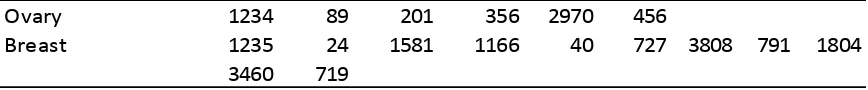
As an example we consider data presented by Hand et al. (1994), see Table 5. Survival times were obtained for 6 patients with ovary cancer and 11 patients with breast cancer (there are no censored observations). Hence, sample sizes are small and unbalanced (for further details see also Cameron and Pauling, 1978). There are no ties, the empirical variances are 1206875 for ovary cancer and 1535038 for breast cancer, which indicates heteroscedasticity.

Table 5: Survival times of cancer patients

Ovary 1234 89 201 356 2970 456

Breast 1235 24 1581 1166 40 727 3808 791 1804

3460 719 Data Source: Hand et al. (1994, p. 255)

There seems to be a tendency for the patients with breast cancer to have larger values. However, the tests are not significant: the p-values are 0.312 for the Welch t test on ranks, 0.320 for the Brunner-Munzel test, and 0.309 for the maximum test based on these two tests (exact permutation tests). This example shows that the maximum test can have a smaller p-value than both single tests. The absolute p-values of the standardized statistics are 1.041/1.100 = 0.946 for Welch t test on ranks, and 0.995/1.089 = 0.914 for the Brunner-Munzel test. Thus, the test statistic of the maximum test is 0.946. The R code written to analyze this example is available from the Dryad Digital Repository.

5. Discussion

Non-normal data are common in practice. Different tests have been proposed for this case, especially for the situation when non-normality is combined with heteroscedasticity. In the literature there is a large variety of studies comparing the different tests. The usual conclusion is that no single test can be recommended for all scenarios (see Introduction). A

possible in a maximum test. For such tests, inference can be based on the permutation null distribution of the maximum, this is useful especially when the distribution of the maximum is not known.

Recently, Neuhäuser (2015) proposed a maximum test for the location-shift model, i.e. when there is no difference in the variances of the two groups. In that case Student’s t test and the Wilcoxon-Mann-Whitney test can be combined. Here, we generalize this idea for the nonparametric Behrens-Fisher problem. We propose a maximum test based on Welch’s t test computed on ranks and the Brunner-Munzel statistic. Our simulation study indicates that the proposed maximum test controls the type I error and stabilizes the power. Thus, we

recommend the maximum test. When applying the maximum test there is no need to select a single test. We also investigated the maximum test with all three considered single tests; however, this maximum test seems to be not better than the recommended test (results not shown).

For large sample sizes, a permutation test can be performed using a simple random sample of permutations. SAS and R programs to carry out permutation tests are given by, for example, Zieffler et al. (2011) and Neuhäuser (2012). Our R code is available from the Dryad Digital Repository.

Finally, it should be noted again that the Welch t test based on ranks, and therefore the recommended maximum test as well, have a heuristic justification only. However the Welch t test based on ranks was investigated and suggested in several studies, the appropriateness and robustness is based on large empirical studies.

References

Berry KJ, Johnston JE, Mielke PW (2014): A chronicle of permutation statistical methods. Springer.

Bradley JV (1978): Robustness? British Journal of Mathematical and Statistical Psychology

31, 144-152.

Brunner E, Munzel U (2000): The nonparametric Behrens-Fisher problem: asymptotic theory and a small sample approximation. Biometrical Journal 42, 17–25.

Brunner E, Munzel U (2013): Nichtparametrische Datenanalyse, unverbundene Stichproben. Springer, 2nd edition.

Cameron E, Pauling L (1978): Supplemental ascorbate in the supportive treatment of cancer: re-evaluation of prolongation of survival times in terminal human cancer. Proceedings

of the National Academy of Science 75, 4538-4542.

Conover WJ, Iman RL (1981): Rank transformation as a bridge between parametric and nonparametric statistics. American Statistician 35, 124–129.

Cribbie RA, Wilcox RR, Bewell C, Keselman HJ (2007): Tests for treatment group equality when data are nonnormal and heteroscedastic. Journal of Modern Applied Statistical Methods 6, 117-132.

Delaney HD, Vargha A (2002): Comparing several robust tests of stochastic equality with ordinally scaled variables and small to moderate sized samples. Psychological Methods 7, 485-503.

Fagerland MW, Sandvik L (2009): The Wilcoxon-Mann-Whitney test under scrutiny.

Statistics in Medicine 28, 1487–1497.

Grissom RJ (2000): Heterogeneity of variance in clinical data. Journal of Consulting and Clinical Psychology 68, 155-165.

Haidous NH, Sawilowsky (2013): Robustness and power of the Kornbrot rank difference, signed ranks, and dependent samples t-test. American Journal of Applied Mathematics and Statistics 1, 99-102.

Hand DJ, Daly F, Lunn AD, McConway KJ, Ostrowski E (1994): A handbook of small data sets. Chapman & Hall/CRC.

Hollander M, Wolfe DA, Chicken E (2014): Nonparametric Statistical Methods. Wiley, 3rd edition.

Neubert K, Brunner E (2007): A studentized permutation test for the nonparametric Behrens-Fisher problem. Computational Statistics and Data Analysis 51, 5192-5204.

Neuhäuser M (2010): A nonparametric two-sample comparison for skewed data with unequal variances. Journal of Clinical Epidemiology 63, 691–693.

Neuhäuser M (2012): Nonparametric Statistical Tests: A Computational Approach. CRC Press.

Neuhäuser M (2015): Combining the t test and Wilcoxon’s rank sum test. Journal of Applied Statistics 42, 2769-2775.

Neuhäuser M, Hothorn L (2006): Maximum Tests are Adaptive Permutation Tests. Journal of Modern Applied Statistical Methods 5, 317-322.

Nguyen DT, Kim ES, de Gil PR, Kellermann A, Chen YH, Kromrey JD, Bellara A (2016): Parametric tests for two population means under normal and non-normal distributions.

Journal of Modern Applied Statistical Methods 16, 141-159.

Vargha A, Delaney HD (1998): The Kruskal-Wallis Test and Stochastic Homogeneity.

Journal of Educational and Behavioral Statistics 23, 170-192.

Zieffler AS, Harring JR, Long JD (2011): Comparing Groups: Randomization and Bootstrap

A

C

A

C

Supplementary table 1. Simulated type I error rates for α = 1%

level=1% sample size: 10,10

VR: 1:1 1:2 1:4

normal Wrank 0.010 0.013 0.012

BM 0.012 0.014 0.013

MAX 0.012 0.014 0.013

uniform Wrank 0.011 0.012 0.014

BM 0.012 0.012 0.014

MAX 0.012 0.012 0.013

poisson Wrank 0.009 0.014 0.014

BM 0.010 0.014 0.013

MAX 0.009 0.013 0.013

sample size: 10,20

VR: 1:1 1:2 1:4

normal Wrank 0.011 0.010 0.009

BM 0.011 0.009 0.007

MAX 0.011 0.009 0.008

uniform Wrank 0.012 0.009 0.011

BM 0.012 0.007 0.006

MAX 0.011 0.008 0.008

poisson Wrank 0.011 0.012 0.011

BM 0.010 0.010 0.008

MAX 0.011 0.010 0.010

sample size: 20,10

VR: 1:1 1:2 1:4

normal Wrank - 0.015 0.016

BM - 0.015 0.016

MAX - 0.014 0.014

uniform Wrank - 0.017 0.019

BM - 0.017 0.018

MAX - 0.015 0.015

poisson Wrank - 0.016 0.019

BM - 0.015 0.018

level=1% sample size: 10,10

VR: 1:1 1:2 1:4

log-normal Wrank 0.012 0.011 0.016

BM 0.011 0.012 0.015

MAX 0.011 0.012 0.015

exponential Wrank 0.012 0.012 0.017

BM 0.011 0.012 0.015

MAX 0.011 0.012 0.015

sample size: 10,20

VR: 1:1 1:2 1:4

log-normal Wrank 0.010 0.013 0.014

BM 0.010 0.011 0.011

MAX 0.010 0.012 0.013

exponential Wrank 0.012 0.011 0.014

BM 0.012 0.010 0.011

MAX 0.013 0.011 0.012

sample size: 20,10

VR: 1:1 1:2 1:4

log-normal Wrank - 0.016 0.019

BM - 0.016 0.018

MAX - 0.015 0.015

exponential Wrank - 0.014 0.020

BM - 0.015 0.019

Supplementary table 2. Simulated type I error rates for α = 2.5%

level=2.5% sample size: 10,10

VR: 1:1 1:2 1:4

normal Wrank 0.024 0.028 0.030

BM 0.026 0.030 0.029

MAX 0.026 0.030 0.030

uniform Wrank 0.026 0.028 0.034

BM 0.027 0.028 0.030

MAX 0.027 0.029 0.029

poisson Wrank 0.023 0.028 0.030

BM 0.023 0.028 0.028

MAX 0.023 0.028 0.029

sample size: 10,20

VR: 1:1 1:2 1:4

normal Wrank 0.027 0.025 0.024

BM 0.027 0.023 0.019

MAX 0.027 0.025 0.023

uniform Wrank 0.027 0.024 0.032

BM 0.027 0.020 0.021

MAX 0.027 0.023 0.030

poisson Wrank 0.026 0.029 0.028

BM 0.026 0.024 0.022

MAX 0.026 0.027 0.026

sample size: 20,10

VR: 1:1 1:2 1:4

normal Wrank - 0.029 0.032

BM - 0.029 0.031

MAX - 0.028 0.029

uniform Wrank - 0.033 0.038

BM - 0.033 0.037

MAX - 0.031 0.032

poisson Wrank - 0.033 0.037

BM - 0.032 0.035

level=2.5% sample size: 10,10

VR: 1:1 1:2 1:4

log-normal Wrank 0.025 0.025 0.033

BM 0.026 0.027 0.032

MAX 0.027 0.027 0.032

exponential Wrank 0.025 0.026 0.035

BM 0.026 0.029 0.033

MAX 0.026 0.029 0.033

sample size: 10,20

VR: 1:1 1:2 1:4

log-normal Wrank 0.024 0.030 0.035

BM 0.025 0.028 0.026

MAX 0.024 0.029 0.032

exponential Wrank 0.027 0.029 0.034

BM 0.026 0.026 0.026

MAX 0.026 0.028 0.031

sample size: 20,10

VR: 1:1 1:2 1:4

log-normal Wrank - 0.032 0.039

BM - 0.033 0.036

MAX - 0.031 0.034

exponential Wrank - 0.031 0.041

BM - 0.032 0.040

Supplementary table 3. Simulated type I error rates for α = 10%

level=10% sample size: 10,10

VR: 1:1 1:2 1:4

normal Wrank 0.094 0.100 0.113

BM 0.098 0.102 0.110

MAX 0.099 0.104 0.114

uniform Wrank 0.098 0.103 0.112

BM 0.102 0.104 0.105

MAX 0.103 0.107 0.111

poisson Wrank 0.094 0.105 0.111

BM 0.097 0.102 0.102

MAX 0.096 0.105 0.107

sample size: 10,20

VR: 1:1 1:2 1:4

normal Wrank 0.100 0.102 0.108

BM 0.101 0.098 0.091

MAX 0.100 0.104 0.109

uniform Wrank 0.101 0.098 0.121

BM 0.100 0.089 0.098

MAX 0.101 0.100 0.123

poisson Wrank 0.105 0.107 0.113

BM 0.104 0.100 0.097

MAX 0.105 0.107 0.113

sample size: 20,10

VR: 1:1 1:2 1:4

normal Wrank - 0.107 0.116

BM - 0.107 0.109

MAX - 0.105 0.106

uniform Wrank - 0.108 0.126

BM - 0.107 0.114

MAX - 0.103 0.112

poisson Wrank - 0.112 0.117

BM - 0.107 0.113

level=10% sample size: 10,10

VR: 1:1 1:2 1:4

log-normal Wrank 0.098 0.101 0.117

BM 0.104 0.102 0.112

MAX 0.105 0.104 0.118

exponential Wrank 0.095 0.103 0.119

BM 0.100 0.103 0.114

MAX 0.100 0.105 0.118

sample size: 10,20

VR: 1:1 1:2 1:4

log-normal Wrank 0.099 0.110 0.127

BM 0.099 0.104 0.112

MAX 0.100 0.113 0.129

exponential Wrank 0.101 0.112 0.129

BM 0.101 0.107 0.110

MAX 0.101 0.114 0.130

sample size: 20,10

VR: 1:1 1:2 1:4

log-normal Wrank - 0.110 0.125

BM - 0.109 0.119

MAX - 0.104 0.116

exponential Wrank - 0.111 0.129

BM - 0.110 0.122