Multi objective optimisation in inventory planning with supplier selection

Multi-objective Optimisation in Inventory Planning

with Supplier Selection

Seda T¨urk, Ender ¨Ozcan, Robert John

ASAP Research Group, School of Computer Science, University of Nottingham, NG8 1BB, Nottingham, UK

Abstract

Supplier selection and inventory planning are critical and challenging tasks in

Supply Chain Management. There are many studies on both topics and many

solution techniques have been proposed dealing with each problem separately.

In this study, we present a two-stage integrated approach to the supplier

selec-tion and inventory planning. In the first stage, suppliers are ranked based on

various criteria, including cost, delivery, service and product quality using

Inter-val Type-2 Fuzzy Sets (IT2FS)s. In the following stage, an inventory model is

created. Then, an Multi-objective Evolutionary Algorithm (MOEA) is utilised

simultaneously minimising the conflicting objectives of supply chain operation

cost and supplier risk. We evaluated the performance of three MOEAs with

tuned parameter settings, namely NSGA-II, SPEA2 and IBEA on a total of

twenty four synthetic and real world problem instances. The empirical results

show that in the overall, NSGA-II is the best performing MOEA producing high

quality trade-off solutions to the integrated problem of supplier selection and

inventory planning.

Keywords: Interval type-2 fuzzy, Evolutionary computation, Metaheuristic,

Optimisation.

Email addresses: syt@cs.nott.ac.uk(Seda T¨urk),exo@cs.nott.ac.uk(Ender ¨Ozcan),

1. Introduction

In today’s competitive and connected environment, many commercial

or-ganisations value effective management of the flow of materials considering the

relationships between vendors, manufacturers, distribution centres, customers

and other services for success (Thomas & Griffin, 1996). The integration of

all facilities which add value for buyers from the procurement of raw materials

to the distribution of end products can be broadly defined as Supply Chain

Management(SCM) (Thomas & Griffin, 1996; Setak et al., 2012). In SCM, it

is crucial to be working with dependable suppliers and planning the inventory

via efficient allocation of the resources in the supply chain for a competitive

advantage Vonderembse & Tracey (1999). Choosing a supplier can impact on

the cost and the quality of products. Evaluation and selection of suppliers is

a critical issue in a supply chain. On the other hand, inventory planning is an

integrated process handling the inventory across the entire network from

sup-pliers to customers. Miller et al. (2011); Miller & John (2010) pointed out that

the supply chains with well managed inventory considers satisfying the demand,

preventing stock outs and reducing holding costs - where stock is kept in the

store for an undesirable period of time.

In most of the previous work, supplier selection and inventory planning are

treated as separate problems. Moreover, many previous studies on supplier

se-lection focus on fuzzy systems formulating the problem as a Multiple Attribute

Decision Making (MADM) problem and taking the requirements of decision

makers into account as well during the solution process. For example,Chen

et al. (2006); Pattnaik (2011); A.Sarkar & Mohapatra (2006) and Gong (2013)

studied an MADM approach based on Type-1 Fuzzy Sets and Interval Type-2

Fuzzy Sets (IT2FS), respectively. The supplier selection problem can be

formu-lated as a multi-objective problem and so some of the previous work investigated

multi-objective models looking into the trade-off between minimisation of total

cost and lead time (Mastrocinque et al., 2013), minimisation of total cost and

cost, maximisation of customer service quality and capacity (Altiparmak et al.,

2006). A thorough review of previous studies on supplier selection, covering a

variety of exact and (meta)heuristic methods as well as computational

intelli-gence techniques, can be found in (Ho et al., 2010). In this study, we extend the

work of Ordoobadi (2009) in which Type-1 Fuzzy Sets are used to capture the

uncertainty in the decision making process and (Turk et al., 2014) in which it

has been observed that IT2FSs can deal with the linguistic uncertainty better.

Hence, we utilise an Interval Type-2 Fuzzy System for evaluating suppliers.

Inventory management is an integrated process handling the inventory across

the entire network from suppliers to customers. Miller et al. (2011); Miller &

John (2010) pointed out that the supply chains with well managed inventory

considers satisfying the demand, preventing stock outs and reducing holding

costs - where stock is kept in the store for an undesirable period of time. In

order to solve inventory planning problem individually, a range of methods

have been used, including genetic algorithms (Rezaei & Davoodi, 2008),

multi-objective algorithms (Liao et al., 2011; Shankar et al., 2013; Zhang et al., 2016)

and hybrid approaches (Mahnam et al., 2009).

Supplier selection combined with effective inventory planning has been

re-searched by a number of researches (Ghodsypour & Brien, 2001;

Mohamma-ditabar & Ghodsypour, 2014; Parhizkari et al., 2013). Majority of the previous

work treated SCM problems as a single objective problem. Although some

studies considered multiple objectives, the problem was dealt with using an

ap-proach designed for optimising a single objective which was obtained by crashing

multiple objectives into one via some scalarisation method, such as, weighted

sum. However, the weakness of such approaches arises mainly due to their

per-formance sensitivity to varying weights and their inability to obtain multiple

trade-off solutions simultaneously after a run (Kim & de Weck, 2006).

There-fore, in our study, three Multi-objective Evolutionary Algorithms (MOEA)s are

used: NSGA-II, SPEA2 and IBEA. In addition, previously proposed heuristic

optimisation approaches could suffer from premature convergence (Esmin et al.,

a diversity mechanism against this issue are utilised. The third MOEA used in

our study, that is IBEA does not necessitate a diversity preservation method

as the indicators such as hypervolume reportedly performs well across a wide

range of problems (Zitzler & K¨unzli, 2004). Moreover, as far as we know, in

none of the previous work covered above, the parameter settings of search

meth-ods were tuned. Nevertheless, evolutionary algorithms like any other

stochas-tic local search method require setting of algorithmic parameters and selected

setting could have an essential impact on their performance. Identifying the

optimal/best parameter settings for a search algorithm is one of the challenging

tasks in designing an effective solution to the problem in hand (Deb, 2007).

However, in our study, parameters of three evolutionary algorithms are tuned.

Only a few previous studies explored multi-objective supplier selection

in-formed inventory planning. In this study, we investigate a two-stage integrated

solution approach to solve the integrated supply chain problem of supplier

selec-tion and inventory planning. The first component involves solving the supplier

selection problem using an IT2FS. Following that an inventory model is

de-veloped to investigate how supplier risk affects cost. The parameters of three

MOEAs are first calibrated using the Taguchi approach (Taguchi & Yokoyama,

1993). After the tuning parameters of these algorithms, each algorithm with the

best setting is applied to the problem in order to examine the trade-off between

operational cost of a supply chain and risk of suppliers. The performances of

NSGA-II, SPEA2 and IBEA are evaluated using well known metrics on twenty

four different problem instances with different characteristics and sizes, where

four of them are real world problem instances and twenty of them are randomly

generated based on those instances.

This paper is organised as follows. Section 2 introduces Type-2 Fuzzy Logic

(T2FL) and multi-objective optimisation including MOEAs and performance

metrics commonly used in the area. Section 3 provides the problem explanation

and the proposed two-stage solution approach. Section 5 presents the

experi-mental design and computational results. Section 6 discusses the conclusions

2. Background

This section introduces the background for the techniques used as a part

of the proposed approach and provides an overview of related studies in the

scientific literature.

2.1. Type-2 Fuzzy Logic

In many problems, knowledge comprises of objective knowledge which is

the formal description of the problem, i.e., mathematical model and

subjec-tive knowledge which encapsulates the linguistic information. Generally in

mathematical models, subjective knowledge is overlooked (Ross, 2004).

How-ever, Zadeh (1965) overcame this issue by introducing fuzzy sets. Mendel &

John (2002) provided the following list of situations where T1FS could be

in-sufficient for capturing the uncertainty in the problems:

1. Meaning of a word often relates to perception and so it could vary from

one person to another with the perception.

2. Further uncertainty may arise if a group of experts do not agree on the

definition of the consequents of a fuzzy system.

3. The input activating a T1FL system may be noisy, and therefore imprecise.

4. The data used for parameter tuning of a T1FL system could be noisy.

Nevertheless, the 3 dimensional fuzzy sets generated using Type-2 Fuzzy

Sets (T2FS)s are extremely complicated, hence it can not be easily understood

and applied. Because of this complexity, many T2FSs applications have been

modelled using Interval Type-2 Fuzzy Logic Systems (Greenfield et al., 2012).

The difference between T2FSs and IT2FSs is that for IT2FS, the membership

function is an interval. This allows us to cope with uncertainty associated with

the membership grades. We use IT2FS to depict the ambiguity inherent in the

supplier selection problem.

2.1.1. Basic Concepts of IT2FS

In this section, we provide the fundamentals of IT2FS as explained in Mendel

Definition 2.1. (Mendel et al., 2006) In the universe of discourseX, a Type-2

Fuzzy Set ˜Acan be assigned by a Type-2 membership functionµA˜indicated as:

˜

A= ((x, u), µ_A˜(x, u))| ∀x∈X,∀u∈Jx⊆[0,1] (1)

where x ∈ X and u ∈ Jx ⊆ [0,1] in which 0 ≤ µ_A˜(x, u) ≤ 1. The primary

membership function is depicted asJx⊆[0,1]. It is also demonstrated as:

˜

A=

Z

x∈X

Z

u∈Jx

µ_A˜(x, u)/(x, u)Jx⊆[0,1] (2)

whereR R denotes a union over all admissiblexandu.

Definition 2.2. (Mendel et al., 2006) ˜A is defined as a Type-2 Fuzzy Set in

the universe of discourseX expressed by the Type-2 membership functionµ_A˜.

When allµ_A˜(x, u) = 1 for∀x∈X andu∈Jx⊆[0,1], ˜Ais termed an Interval

Type-2 Fuzzy Set depicted as:

˜

A=

Z

x∈X

Z

u∈Jx

1/(x, u)Jx⊆[0,1] (3)

whereJx⊆[0,1], i.e.

Definition 2.3. (Mendel et al., 2006) The IT2FS can be considered as a

partic-ular case of type 2 fuzzy set, where the upper and lower membership functions

are both Type-1 membership functions, respectively. As an example, a

trape-zoidal IT2FS ˜Ai for allx∈X represented by;

˜

Ai= ( ˜AUi ,A˜ L

i) = ((a

u i1, a

u i2, a

u i3, a

u

i4;h1( ˜AUi ), h2( ˜AUi )),

(al_i1, al_i2, al_i3, al_i4;h1( ˜ALi), h2( ˜ALi)) (4)

where hj( ˜AUi ) and hj( ˜ALi) for 1 ≤ j ≤ 2 depict membership values of the

corresponding elementsau

i(j+1)and a

l

i(j+1), respectively (Hu et al., 2013). The

height of each constituent membership function is not explicitly defined as it is

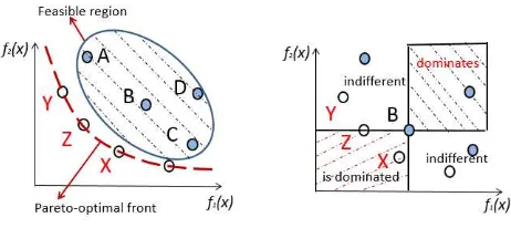
Figure 1: Pareto optimality in objective space(left) and the possible relations of solutions in objective space(right) (Zitzler, 1999).

2.2. Multi-Objective Optimisation

Although, a single objective optimisation technique performs a search to

ob-tain a single solution to a given problem instance, a multi-objective optimisation

is concerned with simultaneous minimisation and/or maximisation of multiple

objectives yielding a set of trade-off solutions which are broadly equivalent

(Zit-zler, 1999).

2.2.1. Basic Concepts of Multi-Objective Optimisation

Generally, multi-objective problems includendecision variables,mobjective

functions andj constraints. Objective functions and constraints are functions

of the decision variables indicated as follows;

minimise f(x)= (f1(x), f2(x), ..., fm(x))

subject to: e(x)= (e1(x), e2(x), ..., ej(x))≤0

where x= (x1, x2, ...xn)∈X,

y= (y1, y2, ..., ym)∈Y

(5)

where x represents decision vector while y is objective vector in X decision

space and Y objective space. Condition ofe(x)≤0 provides the set of feasible

Definition 2.4. Feasible Set (Zitzler, 1999); The set of decision vectors x

which satisfies constraintse(x)is named as the feasible setFS(x):

FS(x)={x∈X|e(x)≤0} (6)

In a single objective optimisation problem, the feasible set is totally ordered

according to objective function f(x): for two solutions x1, x2 ∈ FS(x) either

f1(x)≥f2(x) or f1(x)≤f2(x). The aim is to findf(x)with maximum value.

Nevertheless, when a number of objectives is considered, the feasible set is

partially ordered (Zitzler, 1999).

As an example, in Figure 1, wheref1(x) represents risk,f2(x) denotes cost.

In this example, two objectives generally conflict with each other: high risk

increases the cost while low risk decreases the cost. In Figure 1 on the left,

there are several points as solutions; A, B, C. The solution Z is better than the

solution B with higher performance and lower cost. On the other hand, the

solution Y is better than solution A. Therefore, decision maker can choose an

appropriate solution from the “equivalent” trade-off solutions (Zitzler, 1999).

Definition 2.5. Pareto Dominance (Zitzler, 1999); For any two decision

vectorsx1 andx2;

x1x2 if f1(x)> f2(x)

x1x2 if f1(x)≥f2(x)

x1∼x2 if f1(x)f2(x)∧f2(x)f1(x)

(7)

where x1 x2, x1 x2 and x1 ∼ x2 represent ‘x1 dominates x2’, ‘x1

weakly dominates x2’ and ‘x1 is indifferent tox2’ in a sequence. In Figure 1

on the right, the light grey rectangle area shows the region in objective space

dominated by the solution B while the dark grey rectangles represent the areas

which contain the solution vectors dominating the solution B. All solutions in

the remaining region of the objective space are indifferent to the solution B as

expressed in the last line of Equation 7.

FS(x)is nondominated considering a setPS(x)⊆FS(x)if;

∀xf s∈FS(x):xf sx (8)

All pareto-optimal solutions are referred to as pareto-optimal set where the

corresponding objective vectors form the pareto-optimal front or surface. In

Figure 1, white points demonstrate pareto-optimal solutions: there is no single

optimal solution, but a set of optimal trade-off solutions.

Definition 2.7. Non-dominated Sets and Fronts (Zitzler, 1999);

Let PS(x) ⊆ FS(x), the function p(PS(x)) gives the set of non-dominated

decisions vectors inPS(x).

p(PS(x))={xf s∈FS(x)|xf sis non-dominated consideringFS(x)} (9)

The setp(PS(x))is the non-dominated set inFS(x), the corresponding set of

objective vectorsf(p(PS(x)))is non-dominated front with respect to FS(x).

In addition, the setXp = p(FS(x)) is namely the pareto-optimal set and the

setYp = f(Xp)is called as the pareto-optimal front.

2.3. Multi-objective Evolutionary Algorithms

As the goal in multi-objective optimisation based on a metaheuristic is to

obtain a set of trade-off solutions at the end of the search process for the decision

makers, population based search techniques (which use multiple solutions during

the search), in particular multi-objective evolutionary algorithms (MOEAs) are

naturally preferred. A variety of MOEAs with differing algorithmic components,

such as diversity maintenance, replacement, have been previously proposed and

more can be found in Zitzler & Thiele (1999); Zitzler et al. (2000); Konak et al.

(2006). This work considers three MOEAs: Non-dominated Sorting Genetic

Algorithm II (NSGA-II) (Deb et al., 2002), Strength Pareto Evolutionary

Algo-rithm 2 (SPEA2) (Zitzler et al., 2002), Indicator-Based Evolutionary AlgoAlgo-rithm

(IBEA) (Zitzler & K¨unzli, 2004).

NSGA-II is an elitist MOEA based on a non-dominated sorting method. In

solutions, NSGA-II uses a crowding distance approach to sort individuals (Deb

et al., 2002). Initially, a population P1 of size N is randomly generated and

then thoseN individuals are sorted into different non-domination levels. Then,

an offspring populationQ1of size N is created using the individuals inP1 and

applying crossover and mutation operators with associated probabilities (rates).

P1 andQ1 are merged to formR1 of size 2N which includes elite members of

both parent and offspring populations. All individuals inR1 are sorted into a

number of non-domination levels such asF1, F2 and so on. Starting from F1,

the next populationP2is formed until the size ofP2 achievesN. The crowding

distance approach is used to obtain N member P2 accepting the last levelFn

partially. This process is repeated until to reach a termination criterion (Deb

et al., 2002; Sadeghi et al., 2014; Deb & Jain, 2014).

SPEA2 is also an elitist evolutionary algorithm and works similarly. One

of the main differences is that SPEA2 uses an external archive that consists

of the previously found non-dominated solutions. In addition, SPEA2 uses

an advanced fitness assignment strategy which considers both dominated and

dominating individuals. Moreover, the nearest neighbour density measure is

used in order to maintain the diversity (Zitzler et al., 2002).

IBEA, on the other hand, uses a different approach. The main idea is to

compute the quality of each individual using a predetermined indicator

reduc-ing multiple objectives into a sreduc-ingle “fitness” value. This enables the use of

generic single optimisation methods and so the evolutionary algorithm however

requires maintaining a set of trade-off solutions. In addition, only pairs of

indi-viduals are compared instead of considering entire pareto-front set and diversity

preservation mechanism is not required (Zitzler & K¨unzli, 2004).

2.4. Performance Metrics

The performance of Multi-objective Evolutionary Algorithms are assessed

using various metrics, including the distance of the final pareto set to the global

pareto-optimal front, distribution of the final pareto set with respect to the

Rodemann, 2012). When dealing with multi-objective optimisation problems,

the purpose is to achieve a desirable non-dominated set. However, for a number

of reasons, the assessment of results becomes difficult; i) several solutions are

generated rather than one as in a single objective optimisation problem, ii) a

number of runs needs to be performed to assess the performance of EAs due

to their stochastic nature, iii) different entities, such as, coverage, diversity of

a set of solutions could be measured and used as a guidance during the search

process (Sarker & Coello Coello, 2002). The MOEA performance metrics used

in this study are explained in the following subsections.

2.4.1. Generational Distance (GD)

GD is a method to estimate how far the elements in solutions obtained are

fromP Fglobal set and defined as (Veldhuizen & Veldhuizen, 1999);

GD = 1

n n

X

i=1

dp_i

!1p

(10)

wheren is the number of solutions, di is the Euclidean distance between each

of solutions and the nearest member ofP Fglobal. The value of GD = 0 shows

that all individuals generated are inP Fglobal (Coello et al., 2006), hence lower

the GD better the performance of an algorithm is.

2.4.2. Inverted Generational Distance (IGD)

The IGD metric was first proposed by Czyzak & Jaszkiewicz (1998)

calculat-ing the distance between an objective vector and a reference point. However, the

term itself, “inverted generational distance” was introduced in (Coello Coello &

Reyes Sierra, 2004; Sierra & Coello, 2004).

IGD = 1

m





m

X

j=1

dp_j



 1

p

(11)

where m is the number of vectors in P Fglobal, dj is the Euclidean distance

of p is fixed as 1 in this work. Lower the IGD better the performance of an

algorithm is.

2.4.3. Hypervolume (HV)

Zitzler et al. (2007) proposed a hypervolume indicator (in the literature, it

is found named as ‘Size of the Space Covered’ or ‘Size of Dominated Space’

by Zitzler & Thiele (1999)). The size of a pareto-front set is computed in

objective space by the non-dominated vectors and generally, the definition of

hypervolume indicator is (Brockhoff et al., 2008);

IH(A) =λ

[

a∈A

[f1(a), r1]× ...×[fm(a), rm]

!

(12)

whereIH(A) denotes the hypervolume indicator of a solution setA⊆X and it

is bounded by a reference pointr= (r1, ..., rm)∈Rmwhile it is assumed that

m objective functions f = (f1(x), f2(x), ..., fm(x)) that map solutions x ∈ X

from the decision spaceX to maximize the hypervolume indicatorIH(A). The

Lebesgue measure of a hypervolume set is depicted asλ(HV) where [f1(a), r1]×

[f2(a), r2]× ×[fm(a), rm] is the m-dimensional hypercuboid consisting of all

points that are weakly dominated by the individualabut not weakly dominated

by the reference point. Unlike the other metrics used in this study, higher the

HV better the performance of an algorithm is.

3. Methodology

We propose a two-stage fuzzy based optimisation approach to deal with

the multi-objective integrated supply chain management problem. The first

stage of suppliers are ranked using an IT2FS method while in the second stage,

three MOEAs are studied to solve the supplier selection and inventory planning

problem considering the information provided from the first stage.

3.1. Stage One: Ranking of Suppliers

In this stage, the purpose is to achieve an appropriate approach to rank

Table 1: Linguistic weights of the attributes represented by Interval Type-2 Fuzzy Set (Turk et al., 2014)

Linguistic terms Interval Type-2 Fuzzy Sets

Low importance ((0.0,0.0,0.2,0.3),(0.0,0.0,0.2,0.5))

Moderate importance ((0.3,0.4,0.4,0.5),(0.1,0.4,0.4,0.7))

High importance ((0.5,0.6,0.6,0.7),(0.3,0.6,0.6,0.9))

Very High importance ((0.7,0.8,1.0,1.0),(0.5,0.8,1.0,1.0))

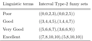
Table 2: Linguistic performance rates represented Interval Type-2 Fuzzy Set (Turk et al., 2014)

Linguistic terms Interval Type-2 fuzzy sets

Poor ((0,0,2,3),(0,0,2,5))

Good ((3,4,4,5),(1,4,4,7))

Very Good ((5,6,6,7),(3,6,6,9))

Excellent ((7,8,10,10),(5,8,10,10))

and assessing the performance of vendors for choosing suppliers Turk et al.

(2015).

3.1.1. Membership Functions

In the study proposed by Ordoobadi (2009), decision makers have examined

two attributes; importance of each criterion to evaluate vendors, performance

rating of suppliers. Turk et al. (2014) developed this work, investigating

uncer-tainty in the proposed problem using IT2FS in order to provide a guideline to

choose an appropriate vendor.

Each criterion is rated using linguistic weights: ‘low importance’, ‘moderate

importance’, ‘high importance’ and ‘very high importance’ (Ordoobadi, 2009).

The numeric scale defined between 0 and 1 corresponds to the fuzzy numbers

shown in Table 1 which indicates the IT2 membership functions used to depict

each of the linguistic weights. Table 1 shows the parameters of a trapezoidal

IT2FS where a trapezoidal is represented by four numbers. In this case, we do

this for both the lover and upper membership functions.

linguis-tic weights: ‘excellent’, ‘very good’, ‘good’ and ‘poor’. The numeric scale

de-termined between 0 and 10 corresponded to the fuzzy numbers of each criterion

value (Ordoobadi, 2009; Turk et al., 2014). The IT2FS are created in the same

manner as denoted previously for modelling the importance weights, and their

values are demonstrated in Table 2 (Turk et al., 2014).

3.1.2. Proposed Method for Ranking Suppliers

After identifying the selection criteria and generating appropriate fuzzy

membership functions, to measure the performance of suppliers and elicit their

ranks, fuzzy mathematical operators are used to calculate a fuzzy score for each

vendor and then to obtain crisp values, these scores are converted through a

type-reduction and defuzzification process. Using these crisp values, the rank

of supplier is achieved. For completeness, further explanation of processes are

given as follows:

Firstly, each importance of criterion chosen by decision makers is used to

generate trapezoidal IT2FSs. These criteria are expressed in linguistic terms

with respect to experts’ perceptions. For example, if a criterion’s importance

weight is ‘high’ then is assigned as ((0.5,0.6,0.6,0.7),(0.3,0.6,0.6,0.9)) as seen

in Table 1. After all criteria are converted into fuzzy numbers, all criteria on the

same branch are multiplied by the previous criterion as indicated in Figure 2.

Letwiindicates the fuzzy importance weight of criterioniwherei= 1,2, ...,10.

For instance,w5 is achieved by multiplying the importance weight of reliability

by the importance weight of the service as:

w8= ((0.5,0.6,0.6,0.7),(0.3,0.6,0.6,0.9))((0.5,0.6,0.6,0.7),(0.3,0.6,0.6,0.9))

= ((0.25,0.36,0.36,0.49),(0.09,0.36,0.36,0.81))

(13)

After all weights are computed in the same manner, trapezoidal IT2FSs for the

performance of vendors are generated in the same way as criteria importance.

And then the aggregate fuzzy set for each vendor is computed by multiplying

the fuzzy performance rates matrix by the fuzzy importance weights as detailed

in Turk et al. (2014). Finally, fuzzy values are converted through Centroid

Figure 2: The criteria and sub-criteria used for selection of suppliers (Ordoobadi, 2009).

3.2. Stage Two: Inventory Planning with Consideration of Supplier Risk

The problem addressed in this study captures features of multi-product

pro-duction while considering the different components. It consists of multiple

sup-pliers, manufacturing plants and potential customers varying from experiment

to experiment. The time for planning is broken down to ‘chunks’ of time. The

first time period depends on what the original stock levels are(Turk et al., 2015).

Other assumptions:

1. Every supply can supply all plants with all components.

2. Every supply and plant has limited capacity for each component and

prod-uct.

3. The cost of the whole operation is the cost of: product, order, transport,

holding of inventory and stock out.

4. Distance between nodes are fixed and known.

Moreover, if an order is not in stock, stock out cost is computed and where

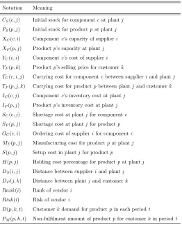
Table 3: Notation for Decision Variables (Turk et al., 2015)

Variable Meaning

PA(p, j, k, t) Amount of productpfrom plantj to customerkin periodt

CA(c, i, j, t) Amount of componentcfrom supplierito plantj in periodt

PI(p, j, t) Inventory of productpat plantj in periodt

CI(c, j, t) Inventory of componentcat plantj in periodt

competitors(Turk et al., 2015).

3.2.1. Multi-objective Model

Presented below is the formulation of the supply chain problem where i, j

andkrepresent a supplier, manufacturing plant and customer, respectively. In

addition, a product, indicated byp, is formed usingc components in discrete

time period denoted by t. Tables 3 and 4 provide the notation to build the

model.

In this work, two objectives are minimised; (i) potential risk endured T R

(Equation 15) as a result of the supplier selection and (ii) the total cost of the

supply chainT C (Equation 14).

The equation 14 computes the total cost summing up the following entities

for each time period/step. In the first row of the equation, the total cost of

inventory is shown for the components and products successively. The

trans-portation cost is accumulated considering the products and then components in

the second and third row, respectively. The next row adds the component order

and setup costs. The manufacturing and shortage costs for each product are

included in the following row. Finally, the total shortage cost for components

and penalty are added to the overall. The penalty cost is incurred when the

Table 4: Notation for Parameters (Turk et al., 2015)

Notation Meaning

CS(c, j) Initial stock for componentcat plantj

PS(p, j) Initial stock for productpat plantj

XC(c, i) Componentc’s capacity of supplieri

XP(p, j) Productp’s capacity at plantj

YC(c, i) Componentc’s cost of supplieri

YP(p, k) Productp’s selling price for customerk

TC(c, i, j) Carrying cost for componentcbetween supplieriand plantj

TP(p, j, k) Carrying cost for productpbetween plantj and customerk

IC(c, j) Componentc’s inventory cost at plantj

IP(p, j) Productp’s inventory cost at plantj

SC(c, j) Shortage cost at plantj for componentc

SP(p, j) Shortage cost at plantj for productp

OC(c, i) Ordering cost of supplierifor componentc

MP(p, j) Manufacturing cost for productpat plantj

S(p, j) Setup cost in plantj for productp

H(p, j) Holding cost percentage for productpat plantj

DS(i, j) Distance between supplieri and plantj

DP(j, k) Distance between plantj and customerk

Rank(i) Rank of vendori

Risk(i) Risk of vendori

D(p, k, t) Customerkdemand for productpin each periodt

PM(p, k, t) Non-fulfilment amount of productpfor customerk in periodt

T C =X

t   X p X j

IP(p, j)×PI(p, j, t) +

X

c

X

j

IC(c, j)×CI(c, k, t)

+X p X j X k

PA(p, j, k, t)×DP(j, k)×TP(p, j, k)

+X c X i X j

CA(c, i, j, t)×DS(i, j)×TC(c, i, j)

+X c X i X j

OC(c, i)×CA(c, i, j, t) +

X p X j X k

S(p, j)×PA(p, j, k, t)

+X p X j X k

MP(p, j)×PA(p, j, k, t) +

X

p

X

j

SP(p, j)×PI(p, j, t)

+XXSC(c, j)×CI(c, j, t) +

XX

PM(p, k, t)YP(p, k)



.

T R=X t

X

c

X

i

X

j

CA(c, i, j, t)×Risk(i) ₍₁₅₎

Equation 15 demonstrates total risk of suppliers with respect to Equation 16

which shows the calculation of a coefficient for the risk of each supplier by

normalising the supplier rank indicated in Table 7.

Risk(i) =

P

iRank(i)

Rank(i) (16)

Equation 17 depicts the supplier capacity for each period and Equation 18 shows

the capacity of the plant for each period.

X

j

CA(c, i, j, t)≤XC(c, i) for∀c, i, t ₍₁₇₎

X

k

PA(p, j, k, t)≤XP(p, j) for∀p, j, t ₍₁₈₎

Equation 19 shows that demand is satisfied by the production units and if, the

production units are not less than the order amount of customer, it is provided

from retailers explained as non-fulfilment amount of a product in Table 4. And

Equation 20 guarantees that the production units are not more than the order

amount of customer. In this model, it is assumed that the first product

com-poses of the first and second components and the second one is produced using

the third and fourth components. Equation 21 describes the inventory-control

constraints for these components and Equation 22 represents inventory-control

constraints for each product.

PM(p, k, t) =D(p, k, t)−

X

j

PA(p, j, k, t) for∀p, k, t. ₍₁₉₎

X

j

X

i

CA(c, i, j, t) +CS(c, j) =

X

k

PA(p, j, k, t) +PI(p, j, t) +CI(c, j, t) ₍₂₁₎

for∀j, twherep= 1 forc={1,2} and wherep= 2 forc={3,4}.

X

j

X

k

PA(p, j, k, t) +

X

j

PS(p, j) =

X

k

D(p, k, t) +X

j

PI(p, j, t)

+X

k

PM(p, k, t) for∀p, t.

(22)

Turk et al. (2015) studied two generic single point based heuristic

opti-misation algorithms, each using a different scalarisation method to solve the

two-objective problem. That study illustrated the multi-objective nature of

the problem testing the proposed approaches on a simple single problem

in-stance. This study extends the previous work and investigates three proper

multi-objective meta-heuristic algorithms to solve the problem with an attempt

to detect the best performing approach.

4. Preliminary Experiments

In this section, we cover the common experimental and algorithmic design,

problem instances and their characteristics as well as preliminary experiments

discussing the results from application of stage one approach and parameter

tuning of NSGA-II, SPEA2 and IBEA.

4.1. Experimental Design

We implemented a fuzzy model and run the stage one approach resulting

with risk of using a particular supplier as explained in Section 3.1. Then this

information is fed into the multi-objective evolutionary algorithms to solve the

integrated problem of supplier selection and inventory planning.

The Jmetal suite (Durillo & Nebro, 2011; Durillo et al., 2010) is used to run

all experiments with the multi-objective evolutionary algorithms. Each trial is

trade-off solutions. A runterminates whenever the 5000 iterations/generations

are exceeded.

A real-valued chromosome representation is used to represent a potential

inventory plan. This plan is encoded into a 4 dimensional array. Each dimension

points out the source node, destination node, component/product and time

period, successively. Each array entry contains a value∈[0,1], representing the

ratio of raw material or goods added to the inventory with respect to the full

capacity of the chosen product at a given source and destination node within a

specific time period. For instance, if the value ofcurrentP lan[3,1,4,2] is 0.5, this

would demonstrate that in period 2, source node 3 is holding 50% of its capacity

of product 4 for destination node 1. The holding can never exceed 100% within

any time period with the proposed encoding. In addition to this, order amount

are decided in certain increments starting from a specified minimum value. For

example, assuming an increment of 100 units and a minimum order of 300 units

for a particular product at a particular node, the orders are restricted to the

increments of 100 starting from 300 (e.g. 300, 400, 500 etc.).

The initial populationis generated randomly. A binary tournament selection

is employed to create a offspring population. Simulated Binary (SBX)Crossover

and PolynomialMutation operator are used by all MOEAs. The common

pa-rameters of SPEA2 and IBEA includepopulation size (P), crossover

probabil-ity (Pc),distribution index for crossover (Dm),distribution index for mutation

(Dc) andarchive size (A). NSGA-II has the same algorithmic control

parame-ters, excluding the archive size. Crossover and mutation probability is utilised

to maintain the frequency of operations. Distribution index for crossover and

mutation are used to control the spread of offspring solutions for which larger

values support “nearer parent” solutions. All the algorithmic control parameters

are tuned for each particular algorithm.

4.2. Problem Instances

In this study, four groups of six problem instances are used, totalling up

Figure 3: Representation of systems consisting of fixed number of suppliers, manufacturing plants and customers, namely 2×2×2, 3×2×3, 3×3×3 and 5×5×5 that 24 instances are derived from.

from S1 to S5 are considered for simplicity. Each group is formed of fixed

number of suppliers, manufacturing plants and customers, namely 2×2×2,

3×2×3, 3×3×3 and 5×5×5 as illustrated in Figure 3. The flow of goods

is also shown in Figure 3 using arrows. The planning horizon contains three

discrete time periods. The production cost, capacity, minimum order

quan-tity, order quantity and initial stock (see Section 3 for more details) are all

parametrised for the instances. Two different settings are used for the problem

instances as summarised in Table 5. The first instances of each group, namely

Inst1, Inst7, Inst13 and Inst19 are real-world problem instances (Miller et al.,

2012) and use a fixed parameter setting. The remaining instances are

ran-domly generated using a certain range for each parameter setting as shown

in Table 6. The problem instances will be made publically available from

Table 5: Configuration of problem instance parameters

Node

Configuration Label

Production Cost Capacity

Minimum Order

Quantities

Order Quantities Initial Stock

Components Products Components Products Components Products Components Products Components Products

Fixed C1 (0.9,0.15,0.3,0.5) (0.5,0.2) 1000 1000 100 100 100 100 250 250

Random C2 [0.20,0.80] [0.20,0.80] [500,1000] [500,1000] [50,200] [50,200] [10,50] [10,50] [0,500] [0,500]

Table 6: Characteristics of the problem instances (S: the number of suppliers, P: the number of manufacturing plants, C: the number of customers, CO: configuration)

Inst S P C CO Inst S P C CO Inst S P C CO Inst S P C CO

Inst1 2 2 2 C1 Inst7 3 2 3 C1 Inst13 3 3 3 C1 Inst19 5 5 5 C1

Inst2-7 2 2 2 C2 Inst8-13 3 2 3 C2 Inst14-19 3 3 3 C2 Inst20-24 5 5 5 C2

4.3. Results from Ranking of Suppliers

Although the overall two-stage approach operates in an integrated manner,

we report the results from stage one separately for the ease of empirical analysis.

The stage one fuzzy method for ranking of relevant suppliers for each instance

is executed as explained in Section 3.1, yielding an output of score, ranking and

risk for each supplier as shown in Table 7. Depending on the number of

sup-pliers in the associated problem instance, the results obtained from the IT2FS

approach for the relevant suppliers are used in the next stage. For example,

considering Inst1, whereS = 2, associated risk values for S1 and S2 are fed into

the stage two approach.

4.4. Parameter Tuning of NSGA-II, SPEA2 and IBEA

The Taguchi orthogonal arrays (Taguchi & Yokoyama, 1993) as a design of

experiments method is used for parameter tuning of each MOEA for improved

performance. We investigated four control parameters for NSGA-II with the

following potential settings: P ∈ {25, 50, 100, 200}, Pc ∈ {0.6,0.7,0.8,0.9}, Dc

and Dm ∈ {5, 10, 15, 20}, and five control parameters for SPEA2 and IBEA

with the addition ofA∈ {25,50,100,200}. The best parameter configuration is

determined based on theL16 Taguchi orthogonal arrays design.

Table 7: Rank and Risk Values of Suppliers for each Instance

Suppliers Crisp Score

Inst1-Inst6 Inst7-Inst18 Inst19-Inst24

Rank Risk Rank Risk Rank Risk

S1 10.88 2 3.28 3 4.90 4 6.60

S2 24.80 1 1.44 1 2.15 1 2.90

S3 17.59 - - 2 3.03 2 4.10

S4 5.96 - - - - 5 12.05

S5 12.56 - - - - 3 5.72

Inst19} and Each of the sixteen parameter settings as provided in Table 8 is

tested using each MOEA applying to the selected problem instances as required

by theL16_{Taguchi orthogonal array design. In order to assess the performance}

of each setting for an MOEA, mean rank (per run), which is obtained by ranking

each setting with respect to hypervolume of the pareto set for each run and then

averaging the ranks of a setting over all runs and problem instances. A lower

value indicates a better performance. As an example in Table 8 the parameter

settings and average rank of three MOEAs are shown.

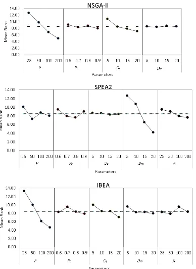
A mean rank for a particular parameter value setting to indicate its main

ef-fect is computed by taking the average of the rank of all runs with that setting on

all instances. For example, let us consider the mean effect of a population size 25

for NSGA-II, which gets computed as (14.87 + 12.14 + 12.27 + 11.00)/4 = 12.60

where this parameter setting corresponds to the first 4 in Table 8. Figure 4

provides the main effects plot indicating the performance of each parameter

value setting. The best configuration for NSGA-II is attained as 200 for P,

0.9 for Pc, 20 for Dc and 10 forDm. Moreover, ANOVA is utilised to analyse

the contribution of each parameter setting on the performance of MOEAs.

Ta-ble 9 summarises the results. The population size as well as distribution index

Table 8: Average rank for three multi-objective algorithms, with a particular parameter con-figuration based on theL16_{Taguchi orthogonal array}

Experiment

number

P Pc Dc Dm A

Average Rank

NSGA-II SPEA2 IBEA

1 25 0.6 5 5 25 14.87 15.8 15.0

2 25 0.7 10 10 50 12.14 11.3 2.6

3 25 0.8 15 15 100 12.27 6.0 10.5

4 25 0.9 20 20 200 11.00 4.8 5.0

5 50 0.6 10 15 200 10.80 13.6 6.4

6 50 0.7 5 20 100 11.84 10.2 8.5

7 50 0.8 20 5 50 8.59 6.3 5.0

8 50 0.9 15 10 25 7.86 5.8 11.6

9 100 0.6 15 20 50 6.71 11.1 7.6

10 100 0.7 20 15 25 4.74 11.4 13.7

11 100 0.8 5 10 200 9.52 6.5 4.8

12 100 0.9 10 5 100 6.09 2.8 11.8

13 200 0.6 20 10 100 3.79 10.1 9.2

14 200 0.7 15 5 200 4.43 9.9 8.0

15 200 0.8 10 20 25 4.53 7.1 12.8

16 200 0.9 5 15 50 6.80 3.3 3.4

Table 9: ANOVA test results for dismissing the contribution of each parameter for MOEAs in terms of percent contribution

MOEAs P Pc Dc Dm A Error Total

NSGA-II 79.28 1.64 17.93 0.12 - 1.03 100%

SPEA2 8.07 4.46 0.17 86.46 0.84 0 100%

IBEA 84.41 2.65 7.82 2.85 2.27 0 100%

settings have significant contribution within a confidence level of 95% on the

performance of NSGA-II, SPEA2 and IBEA, respectively.

In the same manner, the parameters of the other two MOEAs are tuned

and the results achieved are depicted in Table 10. For three instances, the best

parameters setting is performed to confirm that optimum parameters setting is

Figure 4: Main effects plot with mean rank values in three multi-objective algorithms

Table 10: Tuned Parameters of three MOEAs

MOEAs P Pc Dc Dm A

NSGA-II 200 0.9 20 10

-SPEA2 50 0.8 15 20 200

IBEA 200 0.9 20 20 50

three MOEAs outperform all the other setting with the highest hypervolume

values for each instance.

5. Computational Results for Inventory Planning with Consideration

of Supplier Risk

NSGA-II, SPEA2 and IBEA are applied to the twenty four problem instances

the described multi-objective model (See Section 3.2). These MOEAs provide

flexibility for the decision makers enabling them to choose a solution from a set

of ‘equal’ quality solutions reflecting the different levels of trade-off between the

total supplier risk and cost of the supply chain operation.

Table 11 provides the performance comparison of all MOEAs across all

prob-lem instances based on hypervolume, generational distance and inverse

genera-tional distance. We have further performed statistical analysis of results based

on Wilcoxon signed-rank test. In the overall, NSGA-II is the best performing

multi-objective algorithm on average across all instances in terms of all metrics

as shown in Table 11 and we use the following notation in the table.

H0: PN SGA−II > PO

HA: PN SGA−II 6=PO

where H0 represents null hypothesis which asserts that the probability

dis-tributions of the pareto-optimal solutions for NSGA-II are better than other

multi-objective algorithm O and HA represents alternative hypothesis which

the distributions of results differ for NSGA-II and the multi-objective algorithm

considered. The confidence level (significance level) for the non-parametric test

of Wilcoxon signed-rank is set to 95% (p-value under 0.05). The following

nota-tions are used in Table 11. Let us consider two algorithms; NSGA-II versus S,

>(<) indicates that NSGA-II (S) is better than S (NSGA-II) and this

perfor-mance difference is statistically significant within a confidence interval of 95%

and NSGA-II≥S(NSGA-II) ≤S) denotes that NSGA-II (S) performs slightly

better on average than S (NSGA-II) with no statistical significance.

NSGA-II performs significantly better than SPEA2 and IBEA based on

hy-pervolume on all and fourteen out of twenty four instances, respectively. As

for the remaining instances, NSGA-II is slightly better than IBEA on Inst1,

Inst14, Inst16 and IBEA is slightly better than NSGA-II for seven instances.

When the size of problem is enlarged, NSGA-II still provides significantly better

Secondly, with respect to the generational distance, NSGA-II performs

sig-nificantly better than SPEA2 and IBEA for twenty three and fourteen out of

twenty four instances, respectively. For Inst4, SPEA2 is slightly better than

NSGA-II. IBEA is slightly better than NSGA-II over ten instances achieving

lower values of generational distance. NSGA-II provides significantly better

results as the size of the problem grows.

Finally, considering inverse generational distance, NSGA-II outperforms SPEA2

and IBEA for all and seventeen out of twenty four instances, respectively. This

performance variation is statistically significant. IBEA is slightly better than

NSGA-II on seven instances. NSGA-II produces better results when compared

to SPEA2 and IBEA across the last relatively large six instances formed by the

5×5×5 model.

As a sample, we plotted the pareto-front achieved by each MOEA on one

small and one relatively large arbitrarily chosen instances of Inst1 (Figure 5(a))

and Inst19 (Figure 5(b)). As it can be observed from Figure 5(a), NSGA-II and

IBEA produce a wider spread of solutions on the pareto- front when compared

to SPEA2. However, when the size of problem gets larger, the spread of

pareto-front achieved by NSGA-II is better than the others as illustrated in Figure 5(b).

The proposed multi-objective approach provides means to the decision

mak-ers to select a solution among multiple trade-off solutions. A common way of

(automatically) reducing all solutions into a ‘preferable’ reasonable single

solu-tion is detecting the solusolu-tion at the knee point on the pareto-front. We have

used the method presented in (Bechikh et al., 2010) to obtain the a single

solu-tion based on the knee point for the selected problem instances of Inst2, Inst7,

Inst13 and Inst23 from each group of instances. The total cost (T C) and risk

(T R) objectives computed for each such solution to each instance is summarised

in Table 12 which also provides all constituent costs considered.

We have observed that all three MOEAs achieved knee solutions for the

majority of the instances satisfying at least 95% of the customer demand. In

our model, we have merged all cost related entities into a single quantity. The

(a)

(b)

Table 11: Performance comparison of NSGA-II, SPEA2 and IBEA for the two-objective supply chain problem based on three metrics

Inst. HyperVolume

Generational

Distance

Inverse Generational

Distance

NSGA-II SPEA2 IBEA NSGA-II SPEA2 IBEA NSGA-II SPEA2 IBEA

Inst1 Mean 0.7670 > 0.7499 ≥ 0.7640 38,788.8 > 46,646.3 > 38,853.6 80,868.5 > 112,660.2 > 81,344.6 Stnd. 0.007 0.006 0.007 14,576.7 12,136.2 15,011.4 8,937.1 9,624.3 7,693.6

Inst2 Mean 0.7524 > 0.7443 > 0.7522 21,050.6 > 20,784.4

≤ 17,795.4 28,626.2 > 38,201.2 ≤ 28,466.5 Stnd. 0.006 0.006 0.005 7,700.8 10,081.2 8,934.7 3,469.5 8,462.3 6,151.6

Inst3 Mean 0.6798 > 0.6690 ≤ 0.6827 16,155.0 > 23,343.1 > 17,111.6 43,813.0 > 58,283.2 ≤ 42,289.5 Stnd. 0.010 0.009 0.007 7,530.8 13,191.1 8,875.5 13,496.2 11,558.3 11,106.2

Inst4 Mean 0.7118 > 0.6975 > 0.7102 25,067.7

≤ 24,448.8 ≤ 19,732.0 19,232.5 > 27,137.7 ≤ 17,924.7 Stnd. 0.007 0.007 0.007 11,364.0 11,204.9 6,863.9 4,192.6 5,090.4 3,050.3

Inst5 Mean 0.7389 > 0.7261 ≤ 0.7419 29,973.3 > 35,671.8 ≤ 27,021.3 32,679.3 > 44,841.3 ≤ 29,225.3 Stnd. 0.006 0.006 0.007 15,064.0 13,572.4 11,915.6 7,658.2 5,438.9 6,255.5

Inst6 Mean 0.7231 > 0.7139 ≤ 0.7262 19,643.4 > 27,964.4 > 20,936.1 55,117.9 > 65,028.8 ≤ 48,949.9 Stnd. 0.007 0.008 0.008 8,812.7 11,106.9 9,802.2 12,730.1 15,851.2 10,339.5

Inst7 Mean 0.7950 > 0.7807 > 0.7937 73,194.2 > 98,454.5 ≤ 68,210.8 46,447.7 > 71,969.3 > 48,982.1 Stnd. 0.006 0.007 0.005 22,948.1 27,730.4 28,363.9 9,400.8 9,990.9 8,734.1

Inst8 Mean 0.7963 > 0.7890 ≤ 0.7971 51,292.6 > 65,146.7 ≤ 44,247.6 44,620.1 > 65,960.0 > 46,190.9 Stnd. 0.003 0.003 0.003 20,828.8 18,818.9 15,131.2 5,758.3 7,674.1 6,641.7

Inst9 Mean 0.8167 > 0.8099 ≤ 0.8179 41,184.7 > 51,616.5 ≤ 40,559.6 43,557.1 > 63,681.4 > 44,826.9 Stnd. 0.005 0.005 0.004 12,590.0 14,988.6 14,571.4 7,275.9 5,910.5 5,746.3

Inst10 Mean 0.7895 > 0.7820 ≤ 0.7902 50,470.7 > 55,166.1 ≤ 38,779.9 58,429.9 > 81,430.4 ≤ 56,579.2 Stnd. 0.003 0.003 0.004 19,588.8 24,624.4 10,963.8 9,340.2 9,852.3 6,743.8

Inst11 Mean 0.7869 > 0.7803 > 0.7867 37,727.4 > 69,514.3 > 52,187.0 37,494.6 > 58,278.5 > 41,695.2 Stnd. 0.006 0.006 0.004 15,863.5 23,270.4 20,171.1 6,786.3 6,945.6 3,979.2

Inst12 Mean 0.8042 > 0.7964 > 0.8020 34,812.8 > 42,102.8 ≤ 31,673.3 54,967.0 > 79,563.3 > 57,055.7 Stnd. 0.004 0.004 0.004 11,956.9 16,960.9 15,861.2 8,548.7 9,003.0 11,706.3

Inst13 Mean 0.6995 > 0.6844 > 0.6970 65,594.3 > 95,628.9

≤ 62,425.4 101,000.3 > 160,100.0 > 114,165.6 Stnd. 0.006 0.008 0.010 32,003.3 49,046.4 28,715.9 18,361.7 24,095.1 23,797.7

Inst14 Mean 0.6984 > 0.6888 ≥ 0.6983 49,654.3 > 83,012.7 > 54,136.2 49,903.8 > 84,339.3 > 55,597.6 Stnd. 0.004 0.005 0.006 28,079.0 26,854.8 25,396.3 11,236.8 14,165.9 9,390.5

Inst15 Mean 0.7193 > 0.7072 > 0.7164 51,341.3 > 71,084.4 > 53,453.3 56,462.2 > 83,328.4 > 58,799.3 Stnd. 0.003 0.006 0.006 24,657.5 35,538.5 25,487.2 10,613.4 10,306.7 9,442.5

Inst16 Mean 0.6989 > 0.6866 ≥ 0.6988 42,731.6 > 68,389.7 ≤ 41,797.0 65,099.6 > 90,003.3 ≤ 64,687.5 Stnd. 0.007 0.005 0.007 22,905.0 31,368.8 20,417.5 14,635.1 13,199.8 13,303.7

Inst17 Mean 0.6937 > 0.6818 ≤ 0.6940 36,036.0 > 49,477.5 > 43,127.5 47,349.5 > 68,096.5 > 49,781.2 Stnd. 0.006 0.005 0.004 18,783.2 25,172.4 21,004.7 9,664.4 8,401.4 8,492.4

Inst18 Mean 0.7274 > 0.7160 > 0.7248 55,019.1 > 86,545.5 > 59,281.9 38,229.7 > 60,904.3 > 42,108.6 Stnd. 0.006 0.006 0.005 25,699.5 25,917.0 21,631.8 8,980.9 6,022.9 6,144.5

Inst19 Mean 0.7007 > 0.6896 > 0.6994 207,552.1 > 312,479.3 > 255,933.3 202,000.0 > 340,033.3 > 239,933.3 Stnd. 0.005 0.005 0.005 85,716.5 118,172.5 92,387.1 36,561.7 42,619.0 31,514.6

Inst20 Mean 0.7307 > 0.7208 > 0.7271 220,267.2 > 350,882.1 > 305,253.8 95,429.6 > 133,300.0 > 107,733.7 Stnd. 0.004 0.005 0.005 93,103.3 155,641.5 133,632.4 22,586.7 22,557.4 24,639.8

Inst21 Mean 0.7067 > 0.6977 > 0.7049 167,196.4 > 295,800.0 > 192,532.3 196,833.3 > 322,600.0 > 228,033.3 Stnd. 0.004 0.005 0.004 71,342.0 120,451.6 85,651.1 46,431.3 45,895.4 35,427.9

Inst22 Mean 0.7026 > 0.6926 > 0.7049 170,505.4 > 293,433.3 > 167,462.6 138,746.6 > 238,966.7 > 150,369.3 Stnd. 0.006 0.005 0.004 81,088.8 114,547.6 73,489.6 43,605.3 31,957.4 26,484.5

Inst23 Mean 0.7272 > 0.7190 > 0.7258 213,425.3 > 260,961.5 > 178,546.9 129,838.5 > 218,833.3 > 144,924.0 Stnd. 0.004 0.003 0.004 110,600.2 98,614.1 83,908.9 15,750.4 19,206.2 24,959.2

Table 12: Comparison of three MOEAs for two-objective supply chain problem in terms of different cost results which compose the total cost

Inst. Total Risk Total Cost Service Level Batch Cost Production Cost Transportation Cost Stockout Costs Holding Cost

Inst2 NSGA-II 17,220.8 9,648.2 98.24% 450.0 6,571.8 221.3 2,235.1 170.0 SPEA2 15,023.0 10,887.0 98.44% 400.0 7,616.1 195.0 2,505.9 170.0

IBEA 15,282.9 10,907.1 98.44% 420.0 7,544.9 197.2 2,575.0 170.0

Inst7 NSGA-II 30,116.3 21,677.5 95.50% 700.0 17,525.0 443.0 2,034.5 975.0 SPEA2 34,691.0 24,153.5 96.89% 720.0 19,930.0 454.0 2,299.5 750.0

IBEA 37,171.0 22,166.5 98.42% 690.0 18,850.0 405.0 1,871.5 350.0

Inst13 NSGA-II 57,172.0 26,937.5 98.61% 900.0 21,570.0 552.0 3,540.5 375.0 SPEA2 57,558.4 25,355.5 98.03% 910.0 20,365.0 571.0 3,009.5 500.0

IBEA 58,166.6 24,311.0 98.15% 850.0 19,400.0 493.0 3,118.0 450.0

Inst23 NSGA-II 293,495.9 86,074.0 96.92% 2,300.0 64,535.2 2,336.9 14,540.7 2,651.0 SPEA2 301,443.0 88,673.1 96.12% 2,310.0 65,358.0 2,210.0 15,355.5 3,439.0

IBEA 299,561.5 88,115.6 97.88% 2,370.0 66,971.1 2,024.9 14,878.6 1,871.0

costs. For example, Table 12 shows that the SPEA2 solution is better than the

IBEA solution in terms of both total cost and risk. However, service levels and

holding costs are the same and more importantly, SPEA2 solution provides a

better batch, transportation and stock out cost while IBEA solution provides a

relatively better production cost in return worsening the cost for the remaining

items. Considering Inst23, although in the overall, the IBEA solution is better

(dominates) the SPEA2 solution, however again SPEA2 solution is better in

terms of the production cost.

6. Conclusions

In this study, we addressed a supply chain management problem

consider-ing both supplier selection and inventory plannconsider-ing and used an Interval Type-2

Fuzzy System combined with an MOEA. We designed a two-stage approach for

solving the problem; i) suppliers are ranked using IT2FSs, ii) supplier risk and

operational costs for inventory planning are minimised using an MOEA. Hence,

the proposed overall approach is capable of capturing the trade-off between risk

and cost performing a search over the solution space accordingly and providing

a set of ‘equivalent’ solutions. This gives decision makers the flexibility of

choos-ing a solution from a set of trade-off solutions for supply chain management.

three well known MOEAs, namely NSGA-II, SPEA2 and IBEA for solving the

integrated problem. Although, there are several studies on multi-objective

Sup-ply Chain Management (SCM)(Liao et al., 2011; Shankar et al., 2013; Zhang

et al., 2016), to the authors’ knowledge, this is one of the first studies in which

the integrated problem of supplier selection and inventory planning has been

investigated as a multi-objective problem.

Firstly, parameter settings of an MOEA does influence its performance and

in most of the previous studies, parameter tuning appears to be a missing

pro-cess (Liao et al., 2011; Shankar et al., 2013; Zhang et al., 2016). After

param-eter tuning, we used each MOEA at its best performance and tested them on

twenty four problem instances. The empirical results indicate the overall

suc-cess of NSGA-II interacting well with IT2FSs for SCM. All MOEAs achieved

high quality trade-off solutions satisfying the customer demand almost fully in

majority of the cases. A trivial future study could be applying the approach

to new unseen instances possibly even larger than the ones used in this study

and/or changing the decision makers’ supplier related preferences creating more

instances. We provide the problem instances used in this study as a benchmark

along with our implementation of the approach for future research.

The empirical results indicate that there are even more conflicting

objec-tives which can be considered in the solution model and then simultaneously

optimised. Although MOEAs performed reasonably well in this study for the

two-objective problem, this might not be the case when the number of objectives

are increased. Recently, there has been a growing interest into many-objective

(four or more objectives) optimisation considering that existing MOEAs could

struggle in solving such problems (Deb & Jain, 2014) requiring algorithmic

improvement. For example, Deb & Jain (2014) developed NSGA-III as an

extension to NSGA-II with significant chances in the selection operator to

over-come these difficulties. In future work, we intend to investigate the trade-off

all contributing factors to the total cost and risk separately treating each as

a separate objective as well as performances of many-objective approaches to

Acknowledgement

The authors deeply grateful to Simon Miller for assistance with the model

building code.

References

Altiparmak, F., Gen, M., Lin, L., & Paksoy, T. (2006). A genetic algorithm

ap-proach for multi-objective optimization of supply chain networks. Computers

& Industrial Engineering,51, 196 – 215.

A.Sarkar, & Mohapatra, P. (2006). Evaluation of supplier capability and

per-formance: A method for supply base reduction. Journal of Purchasing and

Supply Management, 12, 148 – 163.

Bechikh, S., Ben Said, L., & Gh´edira, K. (2010). Searching for knee regions in

multi-objective optimization using mobile reference points. InProceedings of

the 2010 ACM Symposium on Applied Computing SAC ’10 (pp. 1118–1125).

New York, NY, USA: ACM.

Brockhoff, D., Friedrich, T., & Neumann, F. (2008). Analyzing Hypervolume

Indicator Based Algorithms. In G. Rudolph et al. (Eds.), Conference on

Parallel Problem Solving From Nature (PPSN X) (pp. 651–660). Springer

volume 5199 ofLNCS.

Chen, C.-T., Lin, C.-T., & Huang, S.-F. (2006). A fuzzy approach for supplier

evaluation and selection in supply chain management. International Journal

of Production Economics,102, 289 – 301.

Coello, C. A. C., Lamont, G. B., & Veldhuizen, D. A. V. (2006). Evolutionary

Algorithms for Solving Multi-Objective Problems (Genetic and Evolutionary

Computation). Secaucus, NJ, USA: Springer-Verlag New York, Inc.

Coello Coello, C., & Reyes Sierra, M. (2004). A study of the parallelization

G. Arroyo-Figueroa, L. Sucar, & H. Sossa (Eds.),MICAI 2004: Advances in

Artificial Intelligence(pp. 688–697). Springer Berlin Heidelberg volume 2972

ofLecture Notes in Computer Science.

Czyzak, P., & Jaszkiewicz, A. (1998). Pareto simulated annealing - a

meta-heuristic technique for multiple-objective combinatorial optimization.Journal

of Multi-Criteria Decision Analysis, 7, 34–47.

Deb, K. (2007). Evolutionary multi-objective optimization without additional

parameters. In F. G. Lobo, C. F. Lima, & Z. Michalewicz (Eds.),

Param-eter Setting in Evolutionary Algorithms (pp. 241–257). Berlin, Heidelberg:

Springer Berlin Heidelberg.

Deb, K., & Jain, H. (2014). An evolutionary many-objective optimization

al-gorithm using reference-point-based nondominated sorting approach, part i:

Solving problems with box constraints. IEEE Transactions on Evolutionary

Computation,18, 577–601.

Deb, K., Pratap, A., Agarwal, S., & Meyarivan, T. (2002). A fast and elitist

multiobjective genetic algorithm: Nsga-ii. Evolutionary Computation, IEEE

Transactions on,6, 182–197.

Durillo, J., Nebro, A., & Alba, E. (2010). The jmetal framework for

multi-objective optimization: Design and architecture. In CEC 2010 (pp. 4138–

4325). Barcelona, Spain.

Durillo, J. J., & Nebro, A. J. (2011). jmetal: A java framework for

multi-objective optimization. Advances in Engineering Software,42, 760–771.

Esmin, A. A., Coelho, R. A., & Matwin, S. (2015). A review on particle swarm

optimization algorithm and its variants to clustering high-dimensional data.

Artif. Intell. Rev., 44, 23–45.

Ghodsypour, S., & Brien, C. O. (2001). The total cost of logistics in supplier

constraint. International Journal of Production Economics, 73, 15 – 27.

Supply Chain Management.

Gong, Y. (2013). Fuzzy multi-attribute group decision making method based

on interval type-2 fuzzy sets and applications to global supplier selection.

International Journal of Fuzzy Systems,15.

Greenfield, S., Chiclana, F., John, R., & Coupland, S. (2012). The sampling

method of defuzzification for type-2 fuzzy sets: Experimental evaluation.

In-formation Sciences,189, 77 – 92.

Ho, W., Xu, X., & Dey, P. K. (2010). Multi-criteria decision making approaches

for supplier evaluation and selection: A literature review.Eur. J. Oper. Res.,

202, 16 – 24.

Hu, J., Zhang, Y., Chen, X., & Liu, Y. (2013). Multi-criteria decision

mak-ing method based on possibility degree of interval type-2 fuzzy number.

Knowledge-Based Systems,43, 21–29.

Kim, I., & de Weck, O. (2006). Adaptive weighted sum method for

multiobjec-tive optimization: a new method for pareto front generation. Structural and

Multidisciplinary Optimization,31, 105–116.

Konak, A., Coit, D. W., & Smith, A. E. (2006). Multi-objective optimization

us-ing genetic algorithms: A tutorial.Reliability Engineering and System Safety,

91, 992 – 1007. Special Issue - Genetic Algorithms and ReliabilitySpecial Issue

- Genetic Algorithms and Reliability.

Liao, S.-H., Hsieh, C.-L., & Lai, P.-J. (2011). An evolutionary approach for

multi-objective optimization of the integrated locationˆa¿“inventory

distri-bution network problem in vendor-managed inventory. Expert Systems with

Applications,38, 6768 – 6776.

Mahnam, M., Yadollahpour, M. R., Famil-Dardashti, V., & Hejazi, S. R. (2009).

Supply chain modeling in uncertain environment with bi-objective approach.

Mastrocinque, E., Yuce, B., Lambiase, A., & Packianather, M. (2013). A

multi-objective optimization for supply chain network using the bees algorithm.

International Journal of Engineering Business Management,5, 1–11.

Mendel, J. M., John, R., & Liu, F. (2006). Interval type-2 fuzzy logic systems

made simple. IEEE T. Fuzzy Systems,14, 808–821.

Mendel, J. M., & John, R. B. (2002). Type-2 fuzzy sets made simple. Fuzzy

Systems, IEEE Transactions on,10, 117–127.

Miller, S., Gongora, M., Garibaldi, J., & John, R. (2012). Interval type-2 fuzzy

modelling and stochastic search for real-world inventory management. Soft

Computing,16, 1447–1459.

Miller, S., Gongora, M., & John, R. (2011). Interval type-2 fuzzy modelling

and simulated annealing for real-world inventory management. In Hybrid

Artificial Intelligence Systems 2011 (HAIS2011) 23-25 May, 2011 Wroclaw,

Poland (pp. 231–238).

Miller, S., & John, R. (2010). An interval type-2 fuzzy multiple echelon supply

chain model. Knowledge-Based Systems, 23, 363 – 368. Artificial

Intelli-gence 2009 AI-2009 The 29th{SGAI}International Conference on Artificial

Intelligence.

Mohammaditabar, D., & Ghodsypour, S. H. (2014). A supplier-selection model

with classification and joint replenishment of inventory items. International

Journal of Systems Science,0, 1–10.

Narukawa, K., & Rodemann, T. (2012). Examining the performance of

evolu-tionary many-objective optimization algorithms on a real-world application.

In Proceedings of the 2012 Sixth International Conference on Genetic and

Evolutionary Computing ICGEC ’12 (pp. 316–319). Washington, DC, USA:

IEEE Computer Society.

Ordoobadi, S. M. (2009). Development of a supplier selection model using fuzzy

Parhizkari, M., Amiri, M., & Mousakhani, M. (2013). A multiple criteria

deci-sion making technique for supplier selection and inventory management

strat-egy: A case of multi-product and multi-supplier problem. Decision Science

Letters,2, 185 – 190.

Pattnaik, M. (2011). Supplier selection strategies on fuzzy decision space.

Gen-eral Mathematics Notes,4, 49 – 69.

Rezaei, J., & Davoodi, M. (2008). A deterministic, multi-item inventory model

with supplier selection and imperfect quality. Applied Mathematical

Mod-elling,32, 2106 – 2116.

Ross, T. J. (2004). Fuzzy Logic with Engineering Applications. John Wiley &

Sons.

Sadeghi, J., Sadeghi, S., & Niaki, S. T. A. (2014). A hybrid vendor managed

inventory and redundancy allocation optimization problem in supply chain

management: An nsga-ii with tuned parameters. Computers & Operations

Research,41, 53 – 64.

Sarker, R., & Coello Coello, C. (2002). Assessment methodologies for

multiob-jective evolutionary algorithms. InEvolutionary Optimization (pp. 177–195).

Springer US volume 48 ofInternational Series in Operations Research &

Man-agement Science.

Setak, M., Sharifi, S., & madian, A. A. (2012). Supplier selection and order

allocation models in supply chain management: a review. World Applied

Sciences Journal, 18, 55 – 72.

Shankar, B. L., Basavarajappa, S., Kadadevaramath, R. S., & Chen, J. C.

(2013). A bi-objective optimization of supply chain design and distribution

operations using non-dominated sorting algorithm: A case study. Expert

Sierra, M. R., & Coello, C. A. C. (2004). A new multi-objective particle swarm

optimizer with improved selection and diversity mechanisms. In Proceeding

of the 2004 Congress on Evolutionary Computation (pp. 1–39).

Taguchi, G., & Yokoyama, Y. (1993). Taguchi methods: design of experiments.

TAGUCHI METHODS SERIES. ASI Press.

Thomas, D. J., & Griffin, P. M. (1996). Coordinated supply chain management.

Eur. J. Oper. Res.,94, 1 – 15.

Turk, S., John, R., & ¨Ozcan, E. (2014). Interval type-2 fuzzy sets in supplier

selection. In 14th UK Workshop on Computational Intelligence UKCI2014

(pp. 1–7).

Turk, S., Miller, S., ¨Ozcan, E., & John, R. I. (2015). A simulated annealing

approach to supplier selection aware inventory planning. InIEEE Congress

on Evolutionary Computation, CEC 2015, Sendai, Japan, May 25-28, 2015

(pp. 1799–1806).

Veldhuizen, D. A. V., & Veldhuizen, D. A. V. (1999). Multiobjective

Evolution-ary Algorithms: Classifications, Analyses, and New Innovations. Technical

Report Evolutionary Computation.

Vonderembse, M. A., & Tracey, M. (1999). The impact of supplier selection

criteria and supplier involvement on manufacturing performance. Journal of

Supply Chain Management,35, 33–39.

Zadeh, L. (1965). Fuzzy sets. Information and Control,8, 338 – 353.

Zhang, S., Lee, C. K. M., Wu, K., & Choy, K. L. (2016). Multi-objective

optimization for sustainable supply chain network design considering multiple

distribution channels. Expert Systems with Applications,65, 87 – 99.

Zitzler, E. (1999). Evolutionary algorithms for multiobjective optimization:

Zitzler, E., Brockhoff, D., & Thiele, L. (2007). The hypervolume indicator

revisited: On the design of pareto-compliant indicators via weighted

integra-tion. In S. Obayashi, K. Deb, C. Poloni, T. Hiroyasu, & T. Murata (Eds.),

Evolutionary Multi-Criterion Optimization (pp. 862–876). Springer Berlin

Heidelberg volume 4403 ofLecture Notes in Computer Science.

Zitzler, E., Deb, K., & Thiele, L. (2000). Comparison of multiobjective

evolu-tionary algorithms: Empirical results. Evol. Comput.,8, 173–195.

Zitzler, E., & K¨unzli, S. (2004). Indicator-Based Selection in Multiobjective

Search. In X. Yao et al. (Eds.),Conference on Parallel Problem Solving from

Nature (PPSN VIII)(pp. 832–842). Springer volume 3242 ofLNCS.

Zitzler, E., Laumanns, M., & Thiele, L. (2002). Spea2: Improving the strength

pareto evolutionary algorithm for multiobjective optimization. In

Evolution-ary Methods for Design, Optimisation, and Control (pp. 95–100). CIMNE,

Barcelona, Spain.

Zitzler, E., & Thiele, L. (1999). Multiobjective evolutionary algorithms: a

com-parative case study and the strength pareto approach. Evolutionary