Modeling and impedance analysis of a single DC bus based multiple source multiple load electrical power system

Abstract—The impedance based stability assessment method has been widely used to assess the stability of interconnected systems in different application areas. This paper deals with the source/load impedance analysis of the droop-controlled multiple sources multiple loads system which is a promising candidate in the future more-electric aircraft (MEA). This paper develops a mathematical model of the PMSG-based variable frequency generation system, derives the output impedance of the source subsystem including converter dynamics and shows the effect of parameters variation on source impedance and load impedance. A dynamic droop controller is proposed to provide the active damping to the system. In addition, the impedance analysis is extended to a generalized single bus-based multiple sources multiple loads system in which power losses are also investigated. The aforementioned analytical result is confirmed by experimental results.

Index Terms—Impedance, droop control, constant power load, stability, more electric aircraft, DC power distribution.

I. INTRODUCTION

The more electric aircraft (MEA) concept is one of the major trends in modern aerospace engineering aiming for reduction of the overall aircraft weight, operation cost and environmental impact. Electrically powered systems are employed to replace existing hydraulic, pneumatic and mechanical devices. Hence the onboard installed electrical power increases significantly and this results in challenges in the design of electrical power systems (EPS). Different EPS architectures are currently being studied by the engineering community. At present, the tendency is to replace traditional ac distribution with high-voltage dc. This has several advantages such as increased efficiency, reduced weight and the absence of reactive power compensation devices [1]-[3].

Different power system architectures have been reviewed in [5]. Comparing with ac systems and used primarily on military vehicles and military aircraft, high voltage DC (HVDC) power distribution structure has advantages with respect to the ease of paralleling dc electrical bus bars and integration with loads such as actuators. Fig. 1 shows a promising EPS architecture with multiple generators feeding into a common dc bus. Two generators G1 and G2 connected directly to a shaft in the turbine and output the electrical power directly to the aircraft’s electrical system through the active front-end converters (AFE

Manuscript received April 20, 2016; revised June 19, 2016; accepted July 11, 2016. This work was supported by the CleanSky JTI Project, a FP7 European Integrated Project-http: //www.cleansky.eu.

F. Gao and S. Bozhko are with the Department of Electrical and Electronic Engineering, University of Nottingham, Nottingham, NG7 2RD, U.K. (e-mail: [email protected], [email protected]).

1, AFE 2). Permanent magnet synchronous generators (PMSGs) have been widely used in aerospace applications due to several advantages such as higher efficiency and power density [4]. This variable-frequency system has the advantage such as a simple and reliable configuration in which gear box is not needed between the generator output and the electrical power system.

The parallel operation topology of multiple generators connecting to one engine is promising in the MEA EPS. Appropriate power sharing among the sources is of importance in such multi-source configuration. So far, two methods have been widely used. The first option is master-slave control [6]. The master module acts as a voltage source and works out the current/voltage reference for slaves. However, communication among the parallel modules is needed. System failure can occur if communication fails. Alternatively, appropriate power sharing can also be achieved by employing droop characteristics [7]-[9]. It is much easier for implementation since no communication among the sources is needed. Meanwhile, higher modularity, higher reliability and lower cost of the system can be realized as well.

In addition, as one can see from Fig. 1, there are plenty of loads such as motor drives and power electronic interfaced converters which can be tightly regulated as constant power loads (CPLs). The negative incremental impedance characteristic of CPLs may result in system oscillations and even instability [10]-[12]. Thus, the candidate architecture should be carefully examined for stability in order to guarantee safe EPS operation for a wide range of operation scenarios. The stability of a 270V dc EPS has been analyzed in [13]. A switch reluctance motor is used to investigate the small signal stability. Since it is a standalone generation system, droop control is not used. In terms of small signal stability analysis, two dominant approaches are eigenvalues theorem and the impedance/admittance method. The impedance analysis method has been successfully applied for MEA EPS studies in [14], [15] since it provides an insight into shaping the impedance to assure a stable system. Stability for hybrid ac-dc MEA EPS is investigated in [16], [17] and the influence of some parameters variations on system stability is presented. However, so far there are no published works in regard to the stability analysis of the new power system architecture consisting of multiple sources and multiple loads (see Fig. 1). The main contributions of this paper can be summarized as follows:

Modeling and Impedance Analysis of a Single

DC Bus-based Multiple Sources Multiple Loads

Electrical Power System

G1

G2

270 V DC Bus

DC

DC

DC

AC

Source Load

DC

AC M

28 V DC Bus

LV DC Load

AC Bus

M AC

AC

M AC

DC DC

AC

HV DC Load AFE 1

[image:2.612.57.289.47.204.2]

AFE 2

Fig. 1. Single line diagram of one power system architecture in future MEA. (1) Mathematical equation of source and load impedance of the droop-controlled EPS in future MEA applications is derived taking into account the generator-converter control dynamics. A set of parameters (mainly control parameters) are analyzed in order to specify the power interface characteristic of the cascaded system, such as the output impedance.

(2) A dynamic droop controller, which reshapes the impedance under stability challenging condition, is proposed to provide active damping to the system.

(3) Impedance analysis and subsequent stability investigation has been extended to a generalized power system of multiple loads feeding by parallel sources.

The rest of the paper is organized as follows: In Section II, the control design for the generator-active front end rectifier is presented. The transfer function for dc voltage tracking performance is also derived in the small signal manner. Section III derives the source impedance expression including system dynamics, discusses the source and load impedance for varying parameters and leads to stability assessment. Section IV extends the impedance analysis to a generalized multiple source multiple load dc power system. Experimental validation is shown in Section V in order to confirm the corresponding theoretical results. Section VI draws together the conclusions in this paper.

II. SYSTEM MODELING AND CONTROL DESIGN

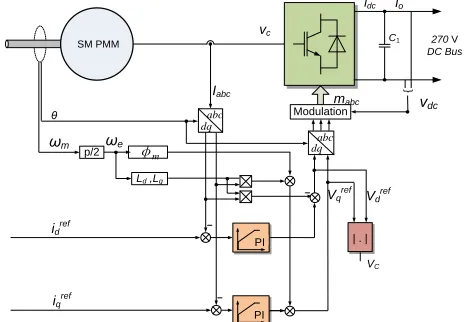
Fig. 2 presents the vector control scheme of the core system. The synchronously rotating reference frame has been widely used to model the PMSG [18]. After transforming the three phase measured currents into the rotating reference frame, conventional PI controllers adjust the stator currents in the dq domain and output dq voltage demands. The voltage demands are inversely transformed into 3-phase modulation indexes for PWM. By controlling the flux in the d-axis and the active power in the q-axis, the PMSG can operate in generating mode within the high speed region. Detailed control design for the PMSG system is discussed in [19].

The dynamic voltage equations of the PMSG can be expressed as follows:

abc dq

mabc

Iabc

PI

PI

abc dq

Ld ,Lq

θ Modulation

iqref

p/2 φ_m

C1

{

SM PMM 270 V

DC Bus

Vdref

Vq ref

| . |

VC

ωm

vdc

vc

idc io

ωe

[image:2.612.325.559.49.210.2]

idref

Fig. 2. Vector control scheme in the single generator-AFE based core system [19].

, d

d s d q

q

q s d d

d d d m q q q

d d

v R i

d t d t

d _d

v R i

d t d t

L i L i

 



 



  



  

  

  

 

  

  

(1)

where vd, vq: d-axis, q-axis component of stator voltage; id, iq:

d-axis, q-axis component of stator current; λd, λq: d-axis, q-axis

component of flux linkage; Rs: stator resistance; ϕm: the flux linkage of permanent magnet; θ:rotor position; Ld, Lq: d-axis,

q-axis inductance. In this study, a surface-mounted permanent magnet machine (SMPMM) is used. The inductance in the d

and q axes are the same and are both expressed as Ls in the

subsequent discussions.

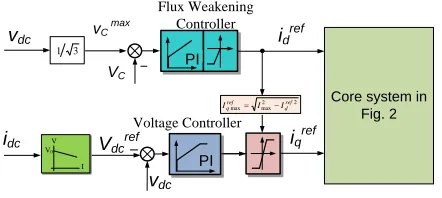
Conventional PI controllers are used to deflux the machine (d-axis) and control the dc voltage (q-axis). The stator current references in d and q axes are obtained from the output of the flux weakening controller and Vdc controller respectively. The

reference of the ac voltage (vc) is dependent on the dc voltage.

The peak convention is used for the transformation from three phase to synchronous rotating frame. The dc voltage reference (vdcref) is dependent on the desired droop characteristic.

A. Inner Current Loop

Considering the inner stator current loop, vd and vq yield:

( )

( )

r e f

d d d C e s q

r e f

q q q C e s d e m

v i i G L i

v i i G L i



  

   

 

   



(2)

where Gc stands for the stator current controller in dq domain.

Inner current loop is designed to be a first-order system and thus, the zero of the PI compensator is set to cancel the pole of the plant. The proportional gain kpc and integral gain kic are

given by:

,

p c c s i c c s

k  L k   R (3)

[image:2.612.373.496.254.349.2]

PI

vC max

Flux Weakening Controller

vdc idc

3 1

PI Voltage Controller

Vdcref V

I

V0

vdc

Core system in Fig. 2

VC

2 2 max max refd ref

q I I

I  

[image:3.612.193.552.44.301.2]

iqref idref

Fig. 3. Outer loop control scheme

B. Flux Weakening Control

In terms of flux weakening control, one can obtain,

m a x

( )

r e f

d c c f w

i  v v G (4)

where vcmax is the maximum phase voltage of the converter and

vc is the ac side phase voltage.

m a x 2 2

, 3 d c

c c d q

v

v  v  v v (5)

where vdc represents the voltage on the local capacitor C1. C. DC Voltage Control

The dc voltage reference Vdcref is obtained by the droop

characteristic (shown in Fig. 4) which is expressed as follows:

r e f

d c o L

V V k I (6)

where k is the droop coefficient, vo is the nominal voltage (270

V in this study) and IL is the load current. The rated voltage of

the main bus is 270 V, but the acceptable steady state range is between 250 V and 280 V as depicted in the standard MIL-STD-704F (see Fig. 5) [20]. If only one source is working in the power system, this control strategy is also feasible for the constant voltage control (droop coefficient k is set to 0).

Fig. 6 shows the control block diagram for the droop-controlled system. According to (1), the linearized q-axis voltage, vq , can be expressed as:

( )

q s s q e s d

v  R  L s i  L i (7) Using the amplitude invariant transformation, the active power can be expressed in dq frame as:

3

( )

2 d d q q

P  v i i v (8)

where vd,vq are theconverter terminal voltages and id, iqare the

ac currents in dq frame.

Assuming the reactive power component equals zero (id =

0), equation (8) can be linearized about an operating point (indicated with the subscript “o”):

3

( )

2 q q o q q o

P  v i  i v (9)

By substituting equation (7) into (9), the active power in small signal can be written as:

I

max

I

dc

V

dc

ref

k

V

o

V

o

lt

ag

e,

V

Time, seconds 0.01 0.02 0.03 0.04 0.05 0.06 0.07 0.08 150

200 250 300 350

280 330

250

Fig. 4. Droop Characteristic. Fig. 5. Voltage requirement for 270 V dc system-MIL-STD-704F.

Vdc

G 1

1 s

  vq

*

q

i

d di

v

3 / 2

dc

v dc

i

o V

L i

Vdc control loop 1

1

C s dc

v k

1

Cs

q

i

Fig. 6. Control block diagram for the droop-controlled system.

3

[ ( ( ) ) ]

2

3

( )

2

s s q o q o q e s q o d

s q o s q o q o q

P R L s i v i L i i

L i s R i v i



   

  

(10)

Thus, the control-to-output (Δidc to Δiqref) can be expressed as:

1 .5 ( )

( 1)

q o s s q o q o

d c

r e f

q d c o

i L s R i v i

i V s

 



 (11)

The control-to-output (Δvdc to Δiqref) transfer function Gp_V(s)

yields,

_

1 .5 ( )

( )

( 1)

q o s s q o q o

d c

P V r e f

q d c o

i L s R i v v

G s

i V C s s

 

 

 (12)

Since vqo is positive and iqo is negative, it can be inferred from (12) that a right half plane (RHP) zero exists in the plant, which can be derived as follows:

s q o q o

q o s

R i v z

i L



  (13)

Due to this RHP zero, a faster bandwidth of the Vdc control

will challenge stability. A PI compensator Gvdc can be used as follows to control the dc voltage,

_

_

i V d c

V d c p V d c

k

G k

s

  (14)

Assuming the 2nd _{order system response with damping ratio ζ} and natural frequency ωVdc, the dc voltage controller gain can

[image:3.612.70.291.47.146.2]

2

_ _

4 2

,

3 3

V d c d c d c V d c d c d c

p V d c i V d c

q q

C V C V

k k

E E

  

  (15)

where Eq is the back electromotive force (EMF) of the

machine. Hence, the voltage control dynamics can be expressed as:

_

_

1

V d c P V

d c D y

o V d c P V

G G

v G

v G G

 



(16)

Substituting (12) and (14) into (16), the voltage control dynamics GDy can be obtained as follows:

1 .5 ( ) ( )

( 1) ( ) 1 .5 ( ) ( )

q o s s q o q o p V d c iV d c

D y

o

d c o q o s s q o q o p V d c iV d c

d c o

i L s R i v k s k

G

P

s s V C s i L s R i v k s k

V 

  



     

(17)

If the load disturbance is neglected, it can be inferred that the voltage dynamics are mainly determined by the controller bandwidth instead of the droop coefficient.

III. IMPEDANCE ANALYSIS

To investigate the influence of parameter variation on stability, it is essential to get a clear view of system characteristic with single source before looking into the complex system with multiple sources and multiple loads.

A. Source and Load Impedance

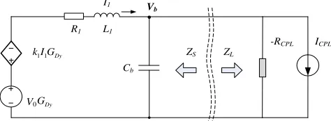
The equivalent circuit for the case of single source operation is presented in Fig. 7. Droop characteristic is implemented by means of an additional current source which is controlled by the main bus voltage Vb. Since the parasitic

capacitance is much smaller than the bus capacitance (Cb) and

the local capacitance (C1), the cabling is represented by series Rc-Lc branch in this section. As mentioned previously, tightly

controlled power electronic converters and motor drives in the EPS can behave like CPLs. As a result the input impedance of the load subsystem can be seen as a negative incremental resistance. As discussed in [21] and [22], a linearized CPL can be approximately expressed by a negative incremental impedance (-RCPL) in parallel with a current source (ICPL).

2

, 2

b C P L

C P L C P L

C P L b

V P

R I

P V

  (18)

where PCPL is the power for the CPL.

The small signal stability of the system is determined by checking the impedance interaction between the source subsystem and load subsystem [23], [24]. Before applying the stability criterion to the cascaded system, it is worth noting that there is a prerequisite for this criterion. The source subsystem and load subsystem must be stable in stand-alone operation. The source impedance in Fig. 6 can be expressed as:

1 1 1

1 1 1

( )

( ) 1

D y

s

b D y

L s R k G Z s

C s L s R k G

 



   (19)

where GDy is the dc voltage tracking performance shown in

(16).

R1 L1

Cb

Vb

ZS ZL

-RCPL I1

V0

ICPL

1 1 Dy k I G

[image:4.612.316.553.49.136.2]

Dy G

Fig. 7. Linearized circuit for cascaded system (source and load subsystem). It is obvious that cable impedance (R1, L1), bus capacitance (Cb) and droop coefficient (k1) will affect the source impedance. Furthermore, parameters such as load power and control bandwidth, which have an effect on GDy, may also

change the output impedance. It is already well known that a large bus capacitance will stabilize the system and increased CPL power will destabilize the system. In the case of a single source feeding a CPL with fixed dc voltage control (k1 = 0), an equilibrium point exists only if the following inequality is satisfied [25],

2

1

4 b C P L

V P

R

 (20)

Neglecting the source dynamics, the overall impedance can be written as

1 1

1 1

2 1 1

1 1

2 2 2

( )

1

( ) / /

( ) (1 )

C P L C P L C P L

b b b

b b b

R L s

Z R L s

P L P R P

C s C L s C R s

V V V



  

    

(21)

In order to rule out any RHP poles to ensure a stable operation, the following conditions should be satisfied:

1 1

1 2 2

( _b C P L) 0 , (1 C P L) 0

b b

L P R P

C R

V V

    (22)

Provided that (20) is satisfied, the second term of (22) is already true. Thus, another upper limit of the CPL can be expressed as:

2 1

1

b b

C P L

C R V P

L

 (23)

Combing (20) and (23), the overall upper limit for the CPL power can be given by:

2 2

1

1 1

m i n ( , )

4

b b b

C P L

V C R V P

R L

 (24)

This paper will focus on the control parameters (droop coefficient, control bandwidth) on source/load impedance. The parameters used for the subsequent bode analysis is listed in Table I.

B. Effect of Vdc Control Bandwidth

It is mentioned at the beginning of this Section that the prerequisite of the impedance method is that both source and load subsystems are stable in standalone condition. Thus, no RHP poles should appear in the impedance expression.

SYSTEM PARAMETERS

Category Parameter Symbol Value

Inner Current Loop

Inner current controller

bandwidth ωc

500 Hz Proportional and integral

gain kpc, kic

6.28, 628.3

DC Link

Cable resistance _Ri 30 mΩ

Cable inductance _Li 1 µH

Local capacitor _Ci 1.6 mF

Bus capacitor Cb 0.8 mF

ac Side ac inductor _LS 2 mH

Fig. 8 shows the layout of the poles of the source impedance (see (19)) with different control bandwidths. It is seen in Fig. 8(a) that a RHP pole appears when the control bandwidth increases to 60 Hz, which indicates that the source subsystem is unstable in standalone condition. When the control bandwidth increases, the proportional (KpVdc) and integral gain (KiVdc) increases correspondingly. The root of the polynomial equation of the denominator of the source impedance in (19) will change and could move from left half plane (LHP) to RHP with the increase of the bandwidth. When the control bandwidth reaches over 60 Hz, one pole of the source impedance is located in the RHP. The source subsystem is unstable in standalone condition and consequently, the overall system (source subsystem + load subsystem) will go unstable as well.

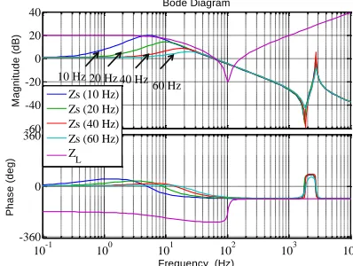
Fig. 9 shows the source impedance with varying Vdc control

bandwidth. It can be seen that the source impedance decreases with the increase of the control bandwidth. The load impedance is invariant to the source control bandwidth. Although the magnitude of the source impedance tends to become smaller when a higher control bandwidth is applied, the standalone subsystem is unstable as shown in Fig. 8.

Therefore, it can be concluded here that a lower control bandwidth would cause the interaction between source and load subsystem, and the phase discrepancy exceeds 180º. As a consequence, the cascaded system is unstable due to this interaction. Alternatively, a very high control bandwidth (e.g., 60 Hz) will result in instability for the source subsystem itself and as a result, the overall system is still unstable.

C. Effect of Droop Coefficient

The effect of droop coefficient variations on the source/load impedances is illustrated in Fig. 10. In terms of the steady state value, the voltage at the main bus will be further reduced under the same load when a higher droop coefficient is applied. As can be inferred from (18), the load impedance will be reduced due to the reduced bus voltage. It can be seen from Fig. 10(b) that the magnitude of the load impedance decreases, which is in alignment with the analysis. Alternatively, the magnitude of the source impedance in low frequency domain increases with the increment of droop coefficient. It can be observed from Fig. 10(b) that when the droop coefficient k is set to 1, the source impedance intersects with the load impedance. Meanwhile, the phase discrepancy between the source and

load impedance is over 180º, leading to an unstable operating point. Overall, it can be concluded that the system stability margin is reduced if a higher droop coefficient is applied.

(a)

(b)

[image:5.612.40.301.61.225.2]

Fig. 8. Pole of the source impedance with respect to different control bandwidth. (a) Overview, (b) Zoomed part of the selected area in (a).

Fig. 9. Source/load impedance with different control bandwidth.

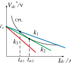
It shows in Fig. 11 that a larger droop constant will cause bigger bus voltage deviation and can even give rise to no intersection point between the source droop curve and CPL hyperbola curve (for example the k3 curve). As a result, no steady-state solution can be found, leading to instability.

As shown in Fig. 11, the V-I characteristic of the main bus can be expressed as

( )

b o i i L

V V  k R I (25)

For the load side, a CPL creates a hyperbolic line which can be expressed as

-2 -1 0 1 2

x 104 -1.5

-1 -0.5 0 0.5 1 1.5

x 104 Pole-Zero Map

Real Axis (seconds-1₎

Im

a

g

in

a

ry

Ax

is

(s

e

c

o

n

d

s

-1)

10 Hz 20 Hz 30 Hz 40 Hz 50 Hz 60 Hz

-600 -500 -400 -300 -200 -100 0 100 -1.5

-1 -0.5 0 0.5 1 1.5

x 104 Pole-Zero Map

Real Axis (seconds-1₎

Im

a

g

in

a

ry

Ax

is

(s

e

c

o

n

d

s

-1)

10 Hz 20 Hz 30 Hz 40 Hz 50 Hz 60 Hz

-60 -40 -20 0 20 40

M

a

g

n

it

u

d

e

(d

B)

10-1 100 101 102 103 104

-360 0 360

Ph

a

s

e

(d

e

g

)

Bode Diagram

Frequency (Hz)

Zs (10 Hz) Zs (20 Hz) Zs (40 Hz) Zs (60 Hz) Z_L

[image:5.612.346.530.85.396.2] [image:5.612.338.537.442.592.2]

(a)

(b)

Fig. 10. Source impedance with different droop coefficients under a 6 kW CPL. (a) Overview of the source/load impedance. (b) Zoomed area of the interaction point.

C P L b L

P  V I (26)

where PCPL is the power of CPL and Io is the load current. The

system can operate normally only if the two curves have an intersection point (equilibrium point). The stable equilibrium point can be derived as follows:

2

2

1

( 4 ( ) ) ,

2 1

( 4 ( ) )

2

b o o i i C P L

L o o i i C P L

i

V V V k R P

I V V k R P

k

   

   

(27)

Considering the existing condition of the operating point in (27), the maximum droop coefficient can be derived as

2

4 o

i i

C P L

V

k R

P

  (28)

Thus, the upper limit of the droop gain can be formulated using (28) and absence of source/load impedance interactions.

D. Proposed Dynamic Droop Controller

In order to enhance the system damping, a dynamic droop coefficient is proposed as:

( ) D

d y

D

k

K s

s

 



 (29)

V

dc*/V

I

dc

/

A Idc1

k

1 CPL

k

3

Vo

k

2

Idc2

Fig. 11. Intersection between the droop-controlled source subsystem and the CPL load subsystem.

PI

vC max

Flux Weakening Controller

vdc

idc

3 1

PI

Voltage Controller Vdcref

vdc

Core system in Fig. 2

VC

2 2 max max

ref d ref

q I I

I  

iqref

id ref

Kdy(s)

Vo

Dynamic Droop

Fig. 12. Proposed dynamic droop controller.

The proposed dynamic droop control is shown in Fig. 12. It can be seen that the proposed dynamic droop controller is employed to replace the conventional fixed droop coefficient. It is virtually a low pass filter with the cutoff frequency

ω

D followed by a gain as the conventional fixed droop coefficient. The principle is to attenuate peak value around the certain resonant frequency region while keeping the other frequency response invariant. The cut off frequency can be designed according to the Vdc control bandwidth with the damping coefficient D.

v d c D

D



  (30)

If the control bandwidth (ωvdc) is set to 10 Hz and the

damping coefficient D is chosen as 2, it can be clearly seen in Fig. 13 that the resonance peak is attenuated by applying the proposed dynamic droop controller. In contrast, the source impedance rarely changes when the droop coefficient is 0.1 or 0.2, as shown in Fig. 14. It can be concluded here that the proposed dynamic droop controller can effectively damp the system under stability challenging condition whilst keeps the performance under lower droop coefficient.

Thus, the system stability cannot be improved by simply increasing Cb. As the eigenvalue sensitivities, with respect to 2

mF or 3 mF Cb, are reduced compared to the case of 1 mF Cb,

it can be inferred that all the modes including the critical modes will gradually converge to a single point in the s-plane.

-60 -40 -20 0 20 40

M

a

g

n

it

u

d

e

(d

B)

10-1 100 101 102 103 104

-270 -180 -90 0 90

Ph

a

s

e

(d

e

g

)

Bode Diagram

Frequency (Hz) Zs(k = 0.1)

Z_L(k = 0.1) Zs(k = 0.2) Z

L(k = 0.2) Zs(k = 0.5) Z_L(k = 0.5) Zs(k = 1) Z_L(k = 1)

Zs (k increases from 0.1 to 1) ZL(k increases from 0.1 to 1)

12 14 16 18 20 22

M

a

g

n

it

u

d

e

(d

B)

100 101

-270 -180 -90 0 90

Ph

a

s

e

(d

e

g

)

Bode Diagram

Frequency (Hz) Zs(k = 0.1)

Z_L(k = 0.1) Zs(k = 0.2) Z_L(k = 0.2) Zs(k = 0.5) Z_L(k = 0.5) Zs(k = 1) Z

L(k = 1)

ZL(k = 1)

[image:6.612.377.501.46.155.2] [image:6.612.75.290.52.358.2] [image:6.612.317.561.193.296.2] [image:6.612.94.244.497.550.2]

(a)

(b)

Fig. 13. Bode plot for the proposed dynamic droop controller for

stability challenging condition (k = 1).

IV. GENERALIZED MULTIPLE SOURCES MULTIPLE LOADS SYSTEM

As one can see from the power system in Fig. 1, multiple sources provide electrical power to the single dc bus to feed multiple loads. Thus, it is worthwhile looking into the stability of the overall system via impedance as well. This section will extends the impedance analysis to a generalized single dc bus-based multiple source multiple load power system.

A. Input Impedance of Multiple Load Subsystem

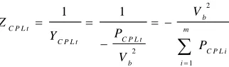
In a modern EPS, there are plenty of power electronic interfaced loads which may behave like CPLs. For the impedance analysis, the parallel CPLs can be modelled in a small signal manner and thus, the total input load admittance of the cumulative CPLs can be expressed as

2

2

1

1 1 _b

C P L t m

C P L t C P L t

C P L i i b

V Z

P Y

P

V _

   



_

(31)

where PCPLi is the power of ith CPL. Hence, similar to the

model of a single CPL in (18), the total CPLs can be represented as a cumulative negative impedance (-RCPLt) in

parallel with a current source (ICPLt).

(a)

(b)

Fig. 14. Bode plot for the proposed dynamic droop controller for smaller droop coefficient: (a) k = 0.1, (b) k = 0.2.

2

1

1

, 2

m

C P L i

b i

C P L t m C P L t

b C P L i

i

P V

R I

V P





  





(32)

Fig. 15 shows the load impedance with the increased number of CPLs. M denotes the number of parallel CPLs. It can be seen that the increased number of CPLs will reduce the magnitude of the load impedance, particularly in low frequency domain. This may result in interactions with the source impedance and as a consequence, cause instability of the system. Thus, in the view of the impedance analysis, it is in alignment with the well-known destabilizing effect of the CPL power.

B. Output Impedance of Multiple Sources Subsystem

The bus voltage with multiple sources can be expressed as follows:

1 1 1

b N N N

V V  I R  V I R (33)

Considering each voltage terminal is droop-controlled and it can be written as:

i o i i

V V I k (34)

Using (34) to substitute the terminal voltage in (33) yields:

1( 1 1) ( )

b o o N N N

V V I R k  V  I R k (35)

-60 -40 -20 0 20

M

a

g

n

it

u

d

e

(

d

B

)

10-1 100 101 102 103 104

-135 -90 -45 0 45 90

P

h

a

se

(

d

e

g

)

Bode Diagram

Frequency (Hz)

Proposed dynamic droop controller Conventional

droop controller

-5 0 5 10 15

M

a

g

n

it

u

d

e

(

d

B

)

100 101

-90 -45 0 45

P

h

a

se

(

d

e

g

)

Bode Diagram

Frequency (Hz)

Proposed dynamic droop controller Conventional

droop controller

-60 -40 -20 0 20

M

a

g

n

it

u

d

e

(d

B)

10-1 100 101 102 103 104

-90 -45 0 45 90

Ph

a

s

e

(d

e

g

)

Bode Diagram

Frequency (Hz) Zs(Conventional Droop)

Zs(Dynamic Droop)

-60 -40 -20 0 20

M

a

g

n

itu

d

e

(d

B)

10-1 100 101 102 103 104

-90 -45 0 45 90

Ph

a

se

(d

e

g

)

Bode Diagram

Frequency (Hz) Zs(Conventional Droop)

[image:7.612.66.275.50.358.2] [image:7.612.341.528.53.358.2] [image:7.612.352.565.403.461.2] [image:7.612.91.252.578.625.2]

[image:8.612.311.560.50.201.2]

Fig. 15. Load impedance with different number of parallel CPLs (dc/dc buck converters).

Reformatting (35), the total load current which is equal to the sum of the branch current can be derived as:

1 1

1

( )

N N

L i o b

i i i i

I I V V

k R

 

  







(36)

Thus, the bus voltage can be written as:

1

1 N

b o L

i i i

V V I

k R



 





(37)

It can be inferred from (37) that the main bus V-I characteristic still follows a droop line which has a stiffer slope compared to individual droop slopes.

Fig. 16 shows the source subsystem consisting of multiple sources and the corresponding impedance model. Similarly as the derivation process in for the single source system in Section III, the overall source impedance can be computed by the ratio of open circuit voltage and short circuit current of the bus bar. Based on Kirchhoff’s circuit laws, open circuit voltage and short circuit current can be calculated as follows:

_

1

1

1

( )

s t N

b

i i i i d y i

Z

C s L s R k G

 



 



(38)

Fig. 17 shows the output impedance of the source subsystem consisting of multiple sources. N stands for the number of multiple sources. Assuming that the power is shared equally among the parallel sources, it can be seen from Fig. 17 that the magnitude of the source impedance reduces with the increased number of parallel sources. The gain in low frequency domain reduces, indicating that at the steady state, the bus voltage deviation is less with the increment of the number of sources.

C. Loss Analysis

Assume that the single source can provide enough power to feed the load, it is worthwhile investigating the optimal operating style to minimize the system losses including distribution losses and converter losses.

DC Bus Cable 1

G1

C1

R1 L1

V2 C2

R2 L2

G2

Cb

Cable 2

Vb

AR2

AR1

Vn Cn

RN LN

GN

Cable N

ARN

I1

I2

IN

Source bank

R1 L1

Cb

Vb

ZS_t

I1

R2 L2

I2

RNLN

IN

(a) _(b)

Source 1

Source 2

Source N V0

1 1 D y1 k I G

V0 2 2 D y2 k I G

V0

N N D y N

k I G

[image:8.612.77.268.56.195.2]

Fig. 16. Modeling of multiple sources. (a) Topology of a single dc bus based multiple sources system. (b) Equivalent circuit.

Fig. 17. Source impedance with different number of parallel sources. Assuming that N sources are operating together in parallel through N parallel AFEs, the line losses can be expressed as follows:

2

1

L l o s s d c d c

P I R

N

  (39)

where Idc is the total dc link current and Rdc is the equivalent dc line resistance connecting from each converter to the bus bar. It can be inferred that the line losses in dc transmission/distribution lines are significantly reduced and further loss reduction could be obtained with more number of parallel sources. Alternatively, the converter losses which take switching loss and conduction loss into consideration can be examined as well. Based on a generalized converter loss expression in [26], [27], a single converter loss can be written as:

2

C l o s s a c a c

P _  a I b I c (40)

The ac side current of each converter is reduced with the increase of the parallel converters. Assuming that the parallel sources share the power equally, the generalized converters loss of N parallel AFEs can be expressed as follows:

2

_

1

*

C l o s s p a r a l l e l a c a c

P a I b I N c

N

    (41)

10-1 100 101 102 103 104

-20 -10 0 10 20 30 40

M

a

g

n

it

u

d

e

(d

B)

Bode Diagram

Frequency (Hz)

M = 1 M = 2 M = 3

-80 -60 -40 -20 0 20

M

a

g

n

it

u

d

e

(d

B)

10-1 100 101 102 103 104

-90 -45 0 45 90

Ph

a

s

e

(d

e

g

)

Bode Diagram

Frequency (Hz) N = 1

[image:8.612.332.549.237.393.2] [image:8.612.48.299.264.358.2]

[image:9.612.328.579.38.366.2]

Fig. 18. Power losses with respect to the number of sources.

where Iac is the total ac side current; a, b, c is the coefficient defined in per unit [27]. Combining the line loss and converter loss shown (39) and (41) respectively, the total loss of N parallel AFEs operation yields,

2 2

_

1

( * )

lo s s p a r a lle l d c d c a c a c

a

P I R I b I N c

N N

    (42)

Fig. 18 shows the power losses (line loss + converter loss) with respect to the number of sources/converters using (39), (41) and (42). It can be seen that the line losses keep reducing with the increase of the number of parallel AFEs. Alternatively, the converter losses reduce to a certain threshold value with the increase of the number of parallel sources initially and then increases with the number of sources. Therefore, with proper selected number of the multiple sources, parallel operation can effectively reduce the losses to some extent.

V. EXPERIMENTAL RESULTS

To perform the aforementioned analysis, the experimental rig (shown in Fig. 19) was built in the lab to support the theoretical analysis of the proposed multi-source paralleled EPS architecture. As depicted in Fig. 20, the experimental setup contains two active front-end converters AFE 1andAFE 2 with a programmable ac source (CHROMA QuadTech 31120) isolated by three-winding step-down transformers (TF 1 and TF 2). Two dc/dc (buck) converters (Chopper 1, Chopper 2) are tightly regulated as CPLs. The experimental system parameters are listed in Table II.

A. Effect of Control Bandwidth

As discussed in Section III-B, due to the existing RHP zero, the Vdc control bandwidth needs to be limited for stable

operation. The experiment with a single converter AFE 1 has been conducted to see the effect of the control bandwidth on system stability. Fig. 21 shows the experimental results with different Vdc control bandwidths when the droop coefficient is

fixed to k1 = 2. It can be seen that with a 8 Hz control bandwidth the system is stable over a CPL power ranging from 0 to 3 kW whilst the system with 80 Hz control bandwidth shows significant oscillation when the load power reaches 3 kW. The result supports the instability discussion in Section III-B.

Fig. 19. Lab prototype.

270 V DC Bus

Cable 1

V1

C1

R1 L1

V2

C2

R2 L2

Cb

Cable 2

Vb

Chopper 2

I2 I1

IL2 AFE 1

AFE 2 TF 1

TF 2 Chroma _{415V/160V, Y/y}

415V/160V, Y/y Lc

Lc

Chopper 1

IL1

Fig. 20. Schematic of the experimental system. TABLE II

EXPERIMENTAL SYSTEM PARAMETERS

Category Parameter Value

Transformer (TF1, TF2) Transformer 415 V/160 V, Y-y

ac Side Inductor (Lin1, Lin2) ac side inductor _{1.2 mH}

dc/dc Converter (Chopper 1, Chopper 2)

Load _{12 Ω}

Inductor _{1.3 mH}

Ratings _{3 kW}

PWM Rectifier (AFE 1, AFE 2)

Switching

frequency 20 kHz Local capacitor _{1.6 mF}

Ratings _{100 kW}

dc Link

dc link capacitor _{0.8 mF} Nominal bus

voltage 270 V

Cable (Rc, Lc) Line resistance 30 mΩ Line inductance _{5 µH}

B. Effect of Droop Coefficient

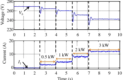
As investigated in Section III-C, the increased droop coefficient will degrade the stability margin. Fig. 22(a) and (b) shows the result when the droop coefficient k1 is set to 1 and 0.1, respectively. Load power demand increases step-wise every 1.5 s. When the load power demand exceeds 3 kW, Chopper 2 is activated. It is shown in Fig. 22(a) that the system is oscillating at a higher power load (6 kW), which indicates

1 2 3 4 5 6 7 8

0 0.005 0.01 0.015 0.02 0.025 0.03 0.035

Number of Sources

L

os

s

(pu)

line loss converter loss total loss

AFE 2

AFE 1

DSP/FPGA Boards Power Supply Oscilloscope

DC Bus

Chopper load

AC Inductor Transformer

Power Supply

Chopper Inductor 2

[image:9.612.68.260.53.205.2] [image:9.612.307.570.420.629.2]

the interaction between the source and load impedance (see Fig. 10). When the droop coefficient is modified to 0.1, the system can work stably with a 6 kW load, as shown in Fig. 22(b). Thus, it confirms that a smaller droop coefficient can obtain more stability margin and the experimental result agrees with the analysis in Section III-C.

(a)

(b)

[image:10.612.326.532.50.366.2]

(c)

Fig. 21. Experimental result of a single AFE with different control bandwidths when k1 = 2. (a) 8 Hz; (b) 20 Hz; (c) 80 Hz.

(a)

[image:10.612.65.278.133.653.2]

(b)

Fig. 22. Experimental result of a single AFE with droop coefficient (a) k1 = 1, (b) k1 = 0.1.

Fig. 23. Experimental result of the proposed dynamic droop controller with 8 Hz control bandwidth (k1 = 2).

C. Effect of Proposed Dynamic Droop Controller

The proposed dynamic droop controller is also tested with the lab prototype. As discussed in Section III.D, two parameters need to be specified for the proposed dynamic droop controller Kdy: damping coefficient D and droop

coefficient k1. The damping coefficient D is set to 2.

For the sake of comparison between the proposed dynamic droop controller and conventional droop controller, the droop coefficient k1 is set to 2 and it is identical to the droop coefficient setting in Fig. 21(a). Fig. 23 shows the experimental result when the proposed dynamic droop controller is activated. In contrast with the result shown in Fig.

-4 -3 -2 -1 0 1 2 3 4 5

220 240 260 280

-4 -3 -2 -1 0 1 2 3 4 5

0 5 10 15

0 0.5 1 1.5 2 2.5 3 3.5 4 4.5 5 240

260

V

ol

tage (V)

280

220

0

Cu

rren

t

(A) 10

5 15

0.5 kW

1 kW 2 kW

3 kW Vb

I₁

Time (s)

0 0.5 1 1.5 2 2.5 3 3.5 4 4.5 5 0 1 2 3 4 5 6 7 8 9 10 0 1 2 3 4 5 6 7 8 9 10

-4 -3 -2 -1 0 1 2 3 4 5

220 240 260 280

-4 -3 -2 -1 0 1 2 3 4 5

0 10 20

Time (s)

0 1 2 3 4 5 6 7 8 9 0 1 2 3 4 5 6 7 8 9 220

240

V

ol

tage (V)

260

0

Current (A)

20

10 280

Vb

I₁

0.5 kW 1 kW

2 kW 3 kW

-4 -3 -2 -1 0 1 2 3 4 5

200 250 300

-4 -3 -2 -1 0 1 2 3 4 5

0 10 20

0 1 2 3 4 5 6 7 8 9

0 1 2 3 4 5 6 7 8 9

Current (A)

0 10 20 200 250 300

V

ol

tage (V)

0.5 kW 1 kW 2 kW 3 kW

Vb

I1

Time (s)

-4 -3 -2 -1 0 1 2 3 4 5

100 200 300 400

-4 -3 -2 -1 0 1 2 3 4 5

0 20 40

0 1 2 3 4 5 6 7 8 9 Time (s)

0 1 2 3 4 5 6 7 8 9

C

ur

rent

(

A

)

0 20 40 200 300

V

ol

tag

e

(V

)

100 400

1 kW 2 kW 3 kW 4 kW 5 kW 6 kW

Vb

I1

Chopper 1 Chopper 1 and 2

-4 -3 -2 -1 0 1 2 3 4 5

250 260 270 280

-4 -3 -2 -1 0 1 2 3 4 5

0 10 20 30

Time (s)

Curr

ent

(A)

0 20 30 270 280

V

ol

tage (V)

260

0 1 2 3 4 5 6 7 8 9

0 1 2 3 4 5 6 7 8 9 250

10

1 kW 2 kW 3 kW 4 kW 5 kW

I1

Vb

6 kW

Chopper 1 Chopper 1 and 2

-4 -3 -2 -1 0 1 2 3 4 5

220 240 260 280

-4 -3 -2 -1 0 1 2 3 4 5

0 10 20

0 1 2 3 4 5 6 7 8 9 10 0 1 2 3 4 5 6 7 8 9 10

V

ol

tage (V)

Cu

rren

t

(A)

Vb

I1

0.5 kW 1 kW 2 kW

3 kW

[image:10.612.332.544.411.550.2]

21(a), it can be seen in Fig. 23 that with the proposed dynamic droop controller, the system is working stably up to 3 kW CPL. Thus, it confirms the effectiveness and damping performance of the proposed dynamic droop approach.

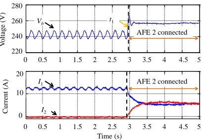
D. Multiple Sources Operation

The parallel operation of AFE 1 and AFE 2 were tested and the result is shown in Fig. 24. Following the result shown in Fig. 21(a), at t = t1, AFE 2 is connected to the bus with the same droop coefficient (k2 = 2) and control bandwidth (8 Hz). It is seen that the bus voltage increases to 258 V and the overall system is stabilized with the parallel operation. The result is consistent with the analysis in Section IV-B (see Fig. 17). The load impedance magnitude increases with the increase of bus voltage whilst the source impedance reduces at the low frequency region. Hence, it demonstrates that in comparison with single source operation, parallel sources can improve the system stability.

VI. CONCLUSION

This paper deals with the stability study of a multi-source multi-load based dc EPS using the impedance approach. A mathematical model of the droop-controlled dc system has been developed and the corresponding source/load impedance has been derived taking into account the converter dynamics. The effect of a set of parameters, e.g., droop coefficient, dc voltage control bandwidth, etc on the source impedance and system stability has been discussed. Furthermore, the impedance analysis has been extended to a generalized system consisting of multiple sources and multiple loads. The impedance of the parallel sources and multiple loads has been analyzed and as a consequence, the stability of the parallel operation has been investigated. The main findings of this paper can be summarized here.

(1) Droop coefficient affects both source and load impedance and consequently, influence system stability. In the voltage droop control strategy, the upper limit of the droop coefficient is determined by two factors. One is the interaction between the source impedance and load impedance. The other is the availability of the steady-state equilibrium point between the source droop curve and CPL hyperbola curve.

(2) A dynamic droop controller is proposed to provide the active damping to the system. The experimental results validate the performance and effectiveness of this proposed method.

(3) Parallel sources can improve the system stability margin. In addition, the losses including converter losses and line losses can be effectively reduced by selecting proper number of parallel source converters.

REFERENCES

[1] X. Liu, P. Wang, and P. C. Loh, “A hybrid ac/dc microgrid and its coordination control,” IEEE Trans. Smart Grid, vol. 2, no. 2, pp. 278– 286, Jun. 2011.

[2] H. Kakigano, Y. Miura, and T. Ise, “Low-voltage bipolar-type dc microgrid for super high quality distribution,” IEEE Trans. Power Electron., vol. 25, no. 12, pp. 3066–3075, Dec. 2010.

[image:11.612.328.533.51.192.2]

[3] D. Salomonsson and A. Sannino, “Low-voltage dc distribution system for commercial power systems with sensitive electronic loads,” IEEE Trans. Power Del., vol. 22, no. 3, pp. 1620–1627, Jul. 2007.

Fig. 24. Experimental result of the multiple sources operation when the AFE 2 is connected (k1 = k2 = 2).

[4] M. E. Haque, Y. C. Saw, and M. M. Chowdhury, “Advanced control scheme for an IPM synchronous generator-based gearless variable speed wind turbine,” IEEE Trans. Sustain. Energy, vol. 5, no. 2, pp.354–362, Apr. 2014.

[5] P. Wheeler and S. Bozhko, “The more electric aircraft: technology and challenges,” IEEE Electrif. Mag., vol. 2, no. 4, pp. 6–12, Dec. 2014. [6] S. K. Mazumder, M. Tahir, and K. Acharya, “Master–slave current

sharing control of a parallel dc–dc converter system over an RF communication interface,” IEEE Trans. Ind. Electron., vol. 55, no. 1, pp. 59–66, Jan. 2008.

[7] S. Anand and B.G. Fernandes, “Modified droop controller for paralleling of dc–dc converters in standalone dc system,” IET Power Electron., vol. 5, no. 6, pp. 782–789, 2012.

[8] J. M. Guerrero, M. Chandorkar, T.-L. Lee, and P. C. Loh, “Advanced control architectures for intelligent microgrids–Part I: Decentralized and hierarchical control,” IEEE Trans. Ind. Electron., vol. 60, no. 4, pp. 1254–1262, Apr. 2013.

[9] J. M. Guerrero, J. C. Vasquez, J. Matas, etc, “Hierarchical control of droop-controlled ac and dc microgrids–A general approach toward standardization,” IEEE Trans. Ind. Electron., vol. 58, no. 1, pp. 158– 172, 2011.

[10] A. Emadi, A. Khaligh, C. Rivetta, and G. Williamson, “Constant power loads and negative impedance instability in automotive systems: Definition, modeling, stability, and control of power electronic converters and motor drives,” IEEE Trans. Veh. Technol., vol. 55, no. 4, pp. 1112–1125, Jul. 2006.

[11] P. Liutanakul, A. Awan, S. Pierfederici, B. Nahid-Mobarakeh, and F. Meibody-Tabar, “Linear stabilization of a dc bus supplying a constant power load: A general design approach,” IEEE Trans. Power Electron., vol. 25, no. 2, pp. 475–488, Feb. 2010.

[12] A. M. Rahimi and A. Emadi, “Active damping in dc/dc power electronic converters: A novel method to overcome the problems of constant power loads,” IEEE Trans. Ind. Electron., vol. 56, no. 5, pp. 1428–1439, May 2009.

[13] L. Han, J. Wang, and D. Howe, “Small-signal stability studies of a 270V dc more-electric aircraft power system,” in Proc. Power Electronics Machines and Drives 2006. The 3rd IET International Conference (PEMD), Apr. 2006, pp. 197–201.

[14] A. Radwan and Y. Mohamed, “Linear active stabilization of converter dominated dc microgrids,” IEEE Trans. Smart Grid, vol. 3, no. 1, pp. 203–216, Mar. 2012.

[15] A. Radwan and Y. Mohamed, “Assessment and mitigation of interaction dynamics in hybrid ac/dc distribution generation systems,”

IEEE Trans. Smart Grid, vol. 3, no. 3, pp. 1382–1393, Sep. 2012. [16] K-N. Areerak, T. Wu, S. V. Bozhko, G. M. Asher, and D. W. P.

Thomas, “Aircraft power system stability study including effect of voltage control and actuators dynamic,” IEEE Trans. Aerosp. Electron. Syst., vol. 47, no. 4, pp. 2574–2589, Oct. 2011.

[17] K-N. Areerak, S. V. Bozhko, G. M. Asher, L. De Lillo, and D. W. P. Thomas, “Stability study for a hybrid ac-dc more-electric aircraft power system,” IEEE Trans. Aerosp. Electron. Syst., vol. 48, no. 1, pp. 329– 347, Jan. 2012.

[18] P. C. Krause, O. Wasynczuk, and S. D. Sudhoff, “Analysis of electric machinery and drive system,” Wiley-IEEE Press, 2002.

-4 -3 -2 -1 0 1 2 3 4 5

220 240 260 280

-4 -3 -2 -1 0 1 2 3 4 5

0 10 20

Time (s)

0 0.5 1 1.5 2 2.5 3 3.5 4 4.5 5 0 0.5 1 1.5 2 2.5 3 3.5 4 4.5 5 240

260

V

ol

tage (V)

280

220

0

Current (A)

20

10 Vb

I₁

I2

t₁

AFE 2 connected

[19] S. Bozhko, S. Yeoh, F. Gao, and C. Hill, “Aircraft starter-generator system based on permanent-magnet machine fed by active front-end rectifier,” in Proc. IECON 2014, 40th Annual Conference of the IEEE, Dallas, USA, Nov. 2014, pp. 2958–2964.

[20] Aircraft Electric Power Characteristics, American Military St. MIL-STD-704F, Mar. 2004.

[21] T. Dragicevic, J. Guerrero, J. Vasquez, and D. Skrlec, “Supervisory control of an adaptive-droop regulated dc microgrid with battery management capability,” IEEE Trans. Power Electron., vol. 29, no. 2, pp. 695–706, Feb. 2014.

[22] P. Karlsson and J. Svensson, “DC bus voltage control for a distributed power system,” IEEE Trans. Power Electron., vol. 18, no. 6, pp. 1405– 1412, Nov. 2003.

[23] A. Riccobono, and E. Santi, “Comprehensive review of stability criteria for DC power distribution systems,” IEEE Trans. Ind. Appl., vol. 50, no. 5, pp. 3525–3535, Sept.-Oct. 2014.

[24] R. D. Middlebrook, “Input filter considerations in design and application of switching regulators,” in Conf. Rec. IEEE IAS Annu. Meeting, 1976, pp. 366–382.

[25] P. Karlsson and J. Svensson, “DC bus voltage control for a distributed power system,” IEEE Trans. Power Electron., vol. 18, no. 6, pp 1405– 1412, Nov. 2003.

[26] A. de la Villa Jaen, E. Acha, and A. G. Exposito, “Voltage source converter modeling for power system state estimation: STATCOM and VSC-HVDC,” IEEE Trans. Power Syst., vol. 23, no. 4, pp. 1552–1559, Nov. 2008.

[27] J. Cao, W. Du, H. Wang, and S. Q. Bu, “Minimization of transmission loss in meshed ac/dc grids with VSC-MTDC networks,” IEEE Trans. Power Syst., vol. 28, no. 3, pp. 3047–3055, Aug. 2013.

Fei Gao received his M.Sc. degree in Electrical Engineering from Shanghai Jiao Tong University, Shanghai, China, in 2010.

From Mar. 2010 to Sep. 2012, he has worked in JiangSu Electric Power Research Institute, State Grid Corporation of China. Currently he is working towards the Ph.D. degree in the Power Electronics, Machines and Control Research Group at The University of Nottingham. His current research interests include modelling and control of electrical power systems, dc microgrids and power system stability.

Serhiy Bozhko (M’96) received his M.Sc. and Ph.D. degrees in electromechanical systems from the National Technical University of Ukraine, Kyiv City, Ukraine, in 1987 and 1994, respectively. Since 2000, he has been with the Power Electronics, Machines and Controls

Research Group of the University of