Object size determines the spatial spread of visual time

rspb.royalsocietypublishing.org

Research

Cite this article:

Fulcher C, McGraw PV, Roach

NW, Whitaker D, Heron J. 2016 Object size

determines the spatial spread of visual time.

Proc. R. Soc. B

283

: 20161024.

http://dx.doi.org/10.1098/rspb.2016.1024

Received: 13 May 2016

Accepted: 4 July 2016

Subject Areas:

cognition, neuroscience

Keywords:

time perception, spatial selectivity,

duration adaptation, visual, size, after-effect

Author for correspondence:

Corinne Fulcher

e-mail: corinne.fulcher@gmail.com

Electronic supplementary material is available

at http://dx.doi.org/10.1098/rspb.2016.1024 or

via http://rspb.royalsocietypublishing.org.

Object size determines the spatial spread

of visual time

Corinne Fulcher

_{, Paul V. McGraw}

_{, Neil W. Roach}

_{, David Whitaker}

and James Heron

1_{Bradford School of Optometry and Vision Science, University of Bradford, BD7 1DP Bradford, UK} 2_{Visual Neuroscience Group, School of Psychology, The University of Nottingham, Nottingham NG7 2RD, UK} 3_{School of Optometry and Vision Sciences, University of Cardiff, Maindy Road, Cathays, Cardiff CF24 4HQ, UK}

CF, 0000-0002-6668-2396; JH, 0000-0003-3857-5056

A key question for temporal processing research is how the nervous system extracts event duration, despite a notable lack of neural structures dedicated to duration encoding. This is in stark contrast with the orderly arrangement of neurons tasked with spatial processing. In this study, we examine the link-age between the spatial and temporal domains. We use sensory adaptation techniques to generate after-effects where perceived duration is either com-pressed or expanded in the opposite direction to the adapting stimulus’ duration. Our results indicate that these after-effects are broadly tuned, extending over an area approximately five times the size of the stimulus. This region is directly related to the size of the adapting stimulus—the larger the adapting stimulus the greater the spatial spread of the after-effect. We construct a simple model to test predictions based on overlapping adapted versus non-adapted neuronal populations and show that our effects cannot be explained by any single, fixed-scale neural filtering. Rather, our effects are best explained by a self-scaled mechanism underpinned by duration selective neurons that also pool spatial information across earlier stages of visual processing.

1. Introduction

Although sub-second timing information is critical to the accuracy of most sen-sory and motor processing, human receptor surfaces do not appear to encode time directly in the way they initiate the analysis of non-temporal features such as pitch, location or temperature. Even at less peripheral locations within the ner-vous system, evidence remains sparse for any neural structures whose primary function relates to the encoding of temporal information. Despite this, we are capable of formulating temporal estimates that, although noisy [1,2] are made see-mingly without conscious effort and form one of the only perceptual metrics that transcends all sensory modalities [3]. This ‘supramodal’ quality has contributed to the dominance of dedicated, modular mechanisms for time perception such as a the pacemaker-accumulator [4–6], oscillator/coincidence-detector [7,8] or memory decay [9] systems. To varying degrees, all of these systems facilitate tem-poral perception by monitoring ongoing background neural activity around the time of stimulus presentation.

In computational terms, centralized models have the attraction of economy in that they avoid the potentially superfluous proliferation of independent, loca-lized timing mechanisms across primary sensory areas. However, the convergence of sensory inputs onto specialized processing modules necessitates an a prioripooling of information across these inputs. It therefore follows that stimulus-specific time perception of any kind presents non-trivial challenges to centralized timing processes. For sub-second duration perception, the possi-bility of multiple localized timing mechanisms is given credence by reports of sensory-specific distortions of perceived duration. For example, perceived

&

visual (but not auditory) duration is compressed around the time of a saccade [10] or via repeated presentation of identical images [11]. More generally, estimates of auditory duration are expanded relative to those for visual stimuli, as well as being significantly less variable [12 –15], in-consistent with a singular central mechanism for the two sensory modalities.

Further examples of sensory-specificity have been revealed by adaptation experiments where exposure to consistent duration information leads to a ‘duration after-effect’ (DAE): adaptation to relatively short/long auditory or visual durations induces perceptual expansion/compression of subsequently viewed/heard intermediate duration stimuli. These repulsion-type after-effects are bidirectional, limited to the adapting stimulus modality and tuned around the adapt-ing duration [16–19]. The neural basis of these effects remains unclear. One possibility is that they reflect a human analogue of the ‘channel-based’ analysis predicted by neurons with bandwidth-limited duration tuning found in a range of neural structures across several amphibian and mammalian species (as recently reviewed in [20]). In the visual domain, the activity of these neurons could form a relatively late-stage, ‘dedicated’, duration-encoding mechanism [21] that—while sensory-specific—could operate at level where basic stimulus features have been pooled to allow selectivity for more com-plex, object-based analysis [22]. Alternatively, if visual event duration forms part of a ‘primal sketch’ [23], duration-tuned neurons would extract duration information alongside low-level stimulus features, prior to any pooling.

Here we address this question by using the orderly relationship between spatial selectivity and visual cortical hierarchy. Specifically, neurons located in extrastriate visual cortex, which perform more complex forms of visual analysis, often inherit pooled inputs from lower-level structures [24,25]. This pooling of information over larger spatial regions supports the analysis of more global image proper-ties, produces receptive fields that are necessarily larger than their inputs and exhibit correspondingly coarser spatial selectivity. Conversely, primary sensory or (even pre-cortical) areas are more closely associated with high degrees of spatial selectivity [26 –31].

By measuring the spatial tuning of DAEs, we are able to show that the effects of adaptation extend well beyond the adapted location. This broad spatial tuning could be consistent with a single, large-diameter receptive field size such as those found in the inferotemporal visual cortex [32]. However, we also show that increasing stimulus size induces a proportional increase in the width of the spatial tuning profiles. We con-struct a simple model based on the degree of overlap between adapted and non-adapted neural populations that allows us to quantify the scale-dependent relationship between size and adaptation spread. We propose DAEs to be a signature of mid-level visual neurons that pool spatial information across proportionally smaller lower-level inputs.

2. Material and methods

(a) Observers

Six observers (three naive) took part in the main experiments (figures 1–3). All observers gave their informed, written consent to participate, and had normal or corrected to normal vision and hearing at the time of the experiment.

(b) Stimuli and apparatus

All visual stimuli were presented on a gamma-corrected Compaq P1220 CRT monitor with a refresh rate of 100 Hz and a resolution of 12801024. This was connected to a 22.26 GHz quad-core Apple Mac Pro desktop computer running Mac OS 10.6.8. All stimuli were generated using MATLAB v. 7.9.0 (Mathworks,

USA) running the Psychtoolbox Extension v. 3.0 (Brainard and Pelli, 1997, www.psychtoolbox.org). The physical durations of all auditory and visual stimuli were verified using a dual-channel oscilloscope. The auditory stimulus was a 500 Hz tone presented through Sennheiser HD 280 headphones. Visual stimuli were isotropic, luminance-defined Gaussian blobs (mean luminance 77 cd m22_{) presented against a uniform grey}

background of 37 cd m22, whose luminance (L) profile was defined as follows:

L¼Lmaxð1þeðx

2_=2s2 stimÞÞ,

whereLmaxis the peak luminance value (set to 94 cd m22) and

sstimis the standard deviation of the Gaussian.

In the initial experiment (figures 2a –cand 3b)s_stimwas set to 18. In subsequent experiments, stimulus size was modified by increasing (s_stim¼1.58, figure 3c) or decreasing (s_stim¼0.58, figure 3a) this value.

(c) Procedure

Observers viewed the visual stimuli binocularly in a quiet, dar-kened room while maintaining fixation on a white 0.078

circular fixation marker presented 5.338to the left of the centre of the screen. Viewing distance was controlled (via chin rest) to ensure one pixel subtended one arc minute. A block of trials began with an initial adapting phase consisting of 100 serially presented visual stimuli. Within a block the duration of these stimuli was fixed at either 160 ms or 640 ms. Interstimulus inter-val (ISI) was randomly jittered between 500 and 1000 ms. The adaptation phase was followed by a further four ‘top up’ adapt-ing stimuli and a subsequent test phase (figure 1) consistadapt-ing of a fixed (320 ms) duration auditory reference stimulus and a variable duration visual test stimulus. Observers then made a two alterna-tive forced choice (2AFC) duration discrimination judgement as to ‘which was longer, flash or beep?’ Visual test stimuli varied in seven approximately logarithmic steps: 240, 260, 290, 320, 350, 390 and 430 ms, which were randomly interleaved within a method of constant stimuli.

Observers responded via key press, which triggered the next top-up and test cycle, until all test durations had been presented 10 times per block of trials. The adapting stimulus was presented at fixation, 58 or 108 to the right of fixation. Test stimuli were either presented at the adapting location or locations providing 58 or 108 adapt –test spatial intervals (figure 1). This provided nine adapt –test spatial configurations (three adapt locationsthree test locations), each of which remained constant within a block of trials. Each adapt –test spatial configuration was repeated for both adapting durations giving a total of 18 conditions. Blocks pertaining to each condition were completed in a random order. Each observer completed three blocks per condition to give 30 repetitions per data point, per observer. In total, data collection lasted approximately 27 h per observer.

The resulting psychometric functions were fitted with a logistic function of the form

y¼ 100

1þeðxPSEu ÞÞ

where PSE represents the point of subjective equality, corre-sponding to the physical test duration that is perceptually equivalent to the 320 ms auditory reference stimulus and u is an estimate of the observer’s duration discrimination threshold

rspb.r

oy

alsocietypublishing.org

Pr

oc.

R.

Soc.

B

283

:

20161024

(half the difference between the values corresponding of 27 and 73% test longer responses). From these functions, PSE values were extracted for each observer for both the 160 and 640 ms adaptation conditions, across each of the nine adapt –test spatial configurations.

(d) Modelling

To aid us in making inferences regarding the spatial scale of duration coding mechanisms, we developed a simple filtering model. We simulated the neural representation (rep) of each stimulus across retinotopic cortex by convolving its horizontal contrast envelope with a Gaussian spatial filter

rep¼eðx2_=2s2

stimÞ eðx

2_=2s2 filtÞ,

where sstim and sfilt are the standard deviations of the

sti-mulus and filter, respectively, and x indicates the spatial distance from the centre of the stimulus/filter (all in degrees of visual angle).

Because both stimulus and filter are Gaussians, rep is itself a Gaussian centred at the location of the stimulus, with a standard deviationsrepgiven by

srep¼

ffiffiffiffiffiffiffiffiffiffiffiffiffiffiffiffiffiffiffiffiffiffiffi

s2

stimþs2filt

q

:

The proportional overlapObetween adapting and test neural representations can be calculated by

O¼2

ð0

1

1

s2 rep

ffiffiffiffiffiffi

2p

p eððxd=2Þ2

=2s2 repÞ_dx,

whered is the centre-to-centre distance between adapting and test stimuli.

The expected DAE was assumed to be a linear function of this overlap

DAE¼kO,

wherekis the peak DAE obtained with identical adapting and test stimuli.

adapt 160 ms duration at fixation

320 ms duration tone

test 320 ms duration at fixation

...or test at 5° eccentricity

...or test at 10° eccentricity time

test phase

adaptation phase

320

ms

320

ms

320

ms

320

ms

160

ms

160

ms

160

ms

160

ms

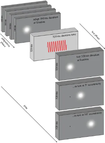
Figure 1.

A schematic showing the adapt – test paradigm. In the adaptation phase, observers view a series of visual stimuli of fixed duration (160 ms in this example) at

one of three possible adapt locations (fixation in this example). In the following test phase, observers make a duration discrimination judgement between a 320 ms

auditory reference duration, and a variable visual test duration (320 ms in this example). The test stimulus may occur at fixation, at 5

8

eccentricity or at 10

8

eccentricity

(constant within a block), forming nine possible adapt – test spatial configurations.

rspb.r

oy

alsocietypublishing.org

Pr

oc.

R.

Soc.

B

283

:

20161024

For each stimulus size, we fitted the spatial filter model to the tuning function relating DAE magnitude to separation, finding the values of srep and k that minimized the sum

of squared residual errors between expected and measured after-effect magnitudes.

3. Results

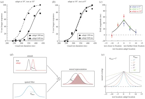
Figure 2ashows sample psychometric functions from a single representative observer. The proportion of responses where the visual test was perceived as longer than the auditory reference is plotted as a function of visual test duration for the condition where both the adapting stimulus and test stimuli were pre-sented at 108 from fixation (i.e. with no spatial separation). Repeated presentations of the 640 ms adapting stimulus (solid black curve, black squares) depresses the number of ‘test longer than reference’ responses, which reflects a perceived com-pression in the duration of the test stimulus: a physical test duration of 377 ms is judged as perceptually equivalent to a physical auditory reference duration of 320 ms. Conversely, the function relating to the 160 ms adaptation condition (dashed curve, black circles) is shifted leftwards, reflecting an expansion of the perceived duration of the test stimulus: a physical test stimulus of 315 ms now has perceptual equivalence with the

reference stimulus. These temporal distortions are consistent with previous reports of bi-directional, repulsive DAEs [17,19].

The extent of the lateral separation between the two func-tions provides a measure of DAE magnitude and can be expressed as the arithmetic difference between PSE values for the two adapting duration conditions

DAE¼PSE640–PSE160,

where PSE640 is the PSE value obtained from the 640 ms

adapting duration and PSE160 is the PSE value obtained

from the 160 ms adapting duration. For the observer shown in figure 2a, DAE¼62 ms when adapting and test durations are both presented at the same location. Of particular interest in this study was to establish how DAE varied during manipulation of the adapt –test spatial interval. Figure 2b

shows psychometric functions for the same observer when the adapting and test stimuli were separated by 108(‘Adapt at 108, test at fixation’). The superimposition of the two func-tions is in stark contrast with the lateral separation shown in figure 2a. This represents a reduction in the effectivity of the adapting stimuli: the perceived duration of the test stimulus shows negligible variation across both adapting durations.

Figure 2cshows data from the same observer where DAE is plotted as a function of all nine adapt–test spatial configur-ations. For all three adapting locations, robust DAEs are

adapt at 10°, test at 0°

0 20 40 60 80 100

200 250 300 350 400 450 adapt at 10°, test at 10°

adapt 160 ms adapt 640 ms

% test longer responses

0 20 40 60 80 100

% test longer responses

visual test duration (ms)

200 250 300 350 400 450 visual test duration (ms)

–20 0 20 40 60 80 100

–15 –10 –5 0 5 10 15

–15 –10 –5 0 5 10 15

adapt at 0° adapt at 5°

adapt at 10°

DAE magnitude (ms)

test closer to fixation test further from fixation

test

adapt

stimuli

spatial filter

neural representation

X

test location-adapt location

0

neural overlap

test location–adapt location 1° 2°

4°

8° 16° sstim1°

srep

sfilter

sfilter

sstim

adapt 160 ms adapt 640 ms

(a) (b) (c)

(d) (e)

Figure 2.

(

a

) Psychometric functions for a single representative observer making duration discrimination judgements following duration adaptation. Circles refer to

the 160 ms adaptation condition and the squares show the 640 ms adaptation condition. In this condition, adapting and test duration were presented at 10

8

temporal to fixation. (

b

) Data from the same observer under identical conditions except for the introduction of a 10

8

spatial interval between adapting and testing

locations. (

c

) A spatial tuning plot showing the variation in duration after-effect (DAE) magnitude across a range of adapt – test spatial configurations (see Methods

and figure 2 for details). An

x

-axis value of zero represents conditions where adapt and test duration were presented at the same spatial location. Positive (negative)

x

-axis values represent conditions in which the test stimulus was presented further from (closer to) fixation than the adapting stimulus. Blue circles represent

conditions where the adapting stimuli were presented at fixation, green circles represent conditions where the adapt location was 5

8

eccentricity and red circles

represent conditions where the adapt location was 10

8

eccentricity. Error bars represent the SEM. (

d

), (

e

) See the main text for details.

rspb.r

oy

alsocietypublishing.org

Pr

oc.

R.

Soc.

B

283

:

20161024

generated by presenting adapt and test stimuli at the same spatial location (figure 2c, central data points). As the adapt– test spatial interval is increased, DAE magnitude shows a progressive decrease, indicating a reduction in the perceptual bias induced by adaptation. This pattern of spatial tuning is manifest for all three adapting locations, as demonstrated by the red, green and blue data points forming a single function. Spatially tuned DAEs are evidence that—at some level— event timing must be segregated into distinct regions of visual space, a finding that could signal the presence of neur-ons that are selective for both the durationandspatial location of a visual event. But what is the spatial scale of duration coding mechanisms? To address this question quantitatively, we developed a simple spatial filtering model based on the assumption that DAEs occur when (and only when) adapting and test stimuli stimulate overlapping neural populations (see Material and methods for details). As illustrated in figure 2d, we first convolved the horizontal contrast profiles of our stimuli with a Gaussian filter corresponding to neural blur, then calculated the proportional overlap between the resulting neural representations of the adapt and test stimuli. The proportion of overlap was then calculated for a range of different adapt –test spatial separations. Figure 2e

shows the resulting spatial tuning functions obtained with a range of neural representation sizes. Application of the model to the individual data shown in figure 2c, revealed a best-fittingsrepof 3.678, which is several multiples of sstim

(the spatial spread of the stimulus). In other words, duration adaptation extends into spatial regions well beyond the physical confines of the adapting stimuli themselves.

A relatively large after-effect spread across space could be consistent with late-stage processing subserved by a coarse, fixed scale of spatial filtering [33]. If this scale (sfilter) is larger

than the stimulus, (sstim—as depicted in figure 2d) the

degree of overlap between adapting and test neural represen-tations (srep) would be similar across modest changes in

stimulus sizes above and below 18. We examined this possi-bility by repeating our experiment using smaller (0.58) and larger (1.58) Gaussian stimuli. Group averaged results for each of the three size conditions are shown in figure 3a–c. Irrespective of stimulus size, DAE magnitude declines system-atically with adapt–test spatial interval; however, the rate of decline varies with stimulus size. This progressive broadening of spatial tuning with increasing stimulus size is summarized in figure 3d, where best-fittingsrepvalues are plotted as a

func-tion ofsstim. In comparison, the dotted lines show a family of

model predictions for different levels of neural blur. Clearly, changes in the spatial tuning of the DAE with stimulus size are not consistent with any fixed scale of spatial filtering.

From the best-fittingsrepvalues, we can work back in our

model to calculate the neural blur of the filter sfilter, which

would have produced this pattern of results. The data predict filter sizes of 2.768, 3.918and 7.868for our three stimulus sizes of 0.58, 18and 1.58. Rather than a fixed level of coarse spatial

0 20 40 60 80 100

0 20 40 60 80 100

0 20 40 60 80 100

–15 –10 –5 0 5 10 15

DAE magnitude (ms)

test further from fixation test closer to fixation

adapt at 0°

adapt at 5°

adapt at 10°

test location–adapt location

–15 –10 –5 0 5 10 15

test further from fixation test closer to fixation

test location–adapt location

–15 –10 –5 0 5 10 15

test further from fixation test closer to fixation

test location–adapt location

sstim1.5°

sstim1°

sstim0.5°

(a) (b) (c)

100

10

1

0.1

0.1 1 10

fixed filter

scaled filter

0°

1° 2°

4°

8° 16° 0°

sstim(°)

srep

(°)

100

10

1

0.1 srep

(°)

0.1 1 10

sstim(°)

sfilter sfilter

1 ×sstim 2 ×sstim

4 ×sstim

5.2 ×sstim 8 ×sstim

(d) (e)

Figure 3.

(

a – c

) Mean spatial tuning plots for the three stimulus sizes (

s

¼

0.5

8

, 1

8

and 1.5

8

), showing DAE magnitude as a function of the spatial separation

between adapt and test locations. Blue circles represent conditions where adaption occurred at 0

8

, green circles represent conditions where adaptation occurred at 5

8

and red circles represent conditions where adaptation occurred at 10

8

. For each adapt – test spatial configuration, stimulus size was held constant between adapting

and test phases. Error bars represent the s.e.m. (

n

¼

6). (

d

), (

e

) See the main text for details.

rspb.r

oy

alsocietypublishing.org

Pr

oc.

R.

Soc.

B

283

:

20161024

filtering, this suggests a ‘self-scaled’ relationship in which the spatial scale of the filter determining after-effect tuning forms a multiple of the spatial scale of the stimulus. Simulations based on this principle are shown in figure 3e where the best-fitting scaled filter is 5.2sstim(figure 3e—black line).

4. Discussion

We sought to investigate the interaction between spatial infor-mation, recent sensory history and the perception of duration. Adaptation techniques were used to generate bidirectional repulsive DAEs, which were tested for their sensitivity to adapt–test changes in spatial location. This sensitivity was found to be coarse: the effects of adaptation spread into a region considerably larger than the adapting stimulus itself (figures 2cand 3b). The size of this region is proportional to the size of the adapting stimulus (figure 3a–c). Our model simulations allowed us to assess our spatial tuning data along-side predictions based on a range of fixed, coarse-scale spatial filters (figure 3d) versus scaled filtering which forms a multiple of stimulus size (figure 3e). Fixed-scale filters were unable to capture the relationship between stimulus size and after-effect spread. Instead, our data are better described by modelling based on the principle that DAEs are generated by a mechanism with self-scaled filtering properties. The effect of this self-scaling is to spread DAEs across an area that is approximately five-times larger than the adapting stimulus.

Broad spatial tuning has practical implications for how adaptation-induced biases are measured. Because duration adaptation do not transfer between sensory modalities [17], our observers judged the perceived duration of a visual test stimulus relative to an auditory reference. An alternative is to use a visual reference that is presented at an unadapted spatial location. However, our data show that it is critical to sufficiently separate the stimuli (particularly if the stimuli themselves are large), otherwise adaptation will influence both the reference and test stimuli during the 2AFC judge-ment. This provides a possible explanation for why robust DAEs have not been reported in experiments using large visual test and reference stimuli presented in relatively close spatial proximity [34].

The spatial tuning reported here contradicts the conclusions of a very recent study where after-effects were generated in one hemisphere (e.g. 108left of fixation) and then tested in the oppo-site hemisphere (e.g. 108right of fixation) [35]. In the Liet al.

study, adapting and test stimuli were always presented at 108 either side of fixation. This raises the possibility that interhemi-spheric communication between corresponding areas of cortical eccentricity (e.g. [36]) could facilitate the transfer of DAEs around an iso-eccentric annulus centred on fixation. This scenario would produce spatial tuning across the annulus’ diameter (as per this study) but not around its circumference (as per the Li et al. study). To investigate this possibility, we repeated our experiment using a 0.58sized stimulus and a 208 adapt–test spatial interval that spanned 108 either side of fixation. The results are shown in the electronic supplementary material, figure S1. In keeping with earlier experiments, (figure 3a–c) all observers show robust DAEs when adapting and test stimuli were both presented 108right of fixation. How-ever, no significant after-effects were generated when adapting stimuli were presented at 108right of fixation and test stimuli were presented 108left of fixation, despite matching eccentricity

across hemispheres. This is consistent with a spatial filtering account of our ‘within-hemisphere’ data (figure 3a), which predicts a negligible (more than 5%) after-effect magnitude for the 0.58sized stimulus across a 208adapt–test spatial interval.

At the opposite extreme to position-invariant accounts of temporal processing, effects are generated when observers view continuous periods of temporally dynamic (flickering or drifting) visual patterns. Subsequently viewed test stimuli typically undergo perceptual compression, (but see [37]) within the same region of the visual field [38,39]. These after-effects show very narrow (approx. 18) spatial tuning [40] and no interocular transfer, leading some to propose an adaptation locus within the magnocellular layers of the LGN ([41], but see [42]). Similarly ‘repetition suppression’ paradigms show that the presentation of two or more identi-cal visual stimuli in close temporal proximity leads the underestimation of the second stimulus’ duration [43]. This effect is exaggerated when the two stimuli share the same orientation and are presented within approximately 28 of each another. Again, these effects have been attributed to mechanisms driven by early striate visual neurons [44].

This group of duration phenomena appear to share some common features: unidirectional (mostly compressive) percep-tual distortion, which is tightly tuned to low-level stimulus characteristics such as spatial location. These features contrast sharply with the DAEs reported here which could suggest that the two types of after-effect (unidirectional, narrowly tuned versus bidirectional, broadly tuned) might be signatures of distinct temporal processing mechanisms.

However, recent advances in our understanding of visual spatial adaptation offer an alternative interpretation. Adaptation to stimulus features such as contrast, temporal frequency, motion and orientation modulates neural activity across a wide range of areas from the retina, to the striate and extrastriate cortices (as recently reviewed in [45]). Neurophysiological advances have revealed an adaptation cascade where the activity at any given site is a product of adaptation intrinsic to neurons at that siteandadaptation inherited from earlier visual areas [46,47]. In some cases [47,48], the ‘downstream’ recipients of ‘upstream’ adaptation are unable to distinguish between adapted and non-adapted inputs, leading to a cumulative superimposition of distinct adaptation effects [49,50].

Could adaptation effects from different levels of neural pro-cessing also occur for temporal information? Because receptive field size increases systematically throughout pre-cortical, stri-ate and extrastristri-ate visual areas [26–30], our broad spatial tuning dictates that bidirectional, repulsive DAEs must orig-inate at a cortical location beyond that responsible for the narrowly tuned, unidirectional effects discussed above. What-ever the relationship between these two after-effects, simple inheritance of earlier adaptation would predict that our repul-sive DAEs should display similarly narrow spatial tuning [24,51]. Instead, our tuning profiles suggest repulsive DAEs are generated by subsequent phase of adaptation that is embo-died with the spatial selectivity of neurons whose larger receptive field size reflects their downstream location [46,52,53]. In this context, the output duration signal from early mechanisms [39,43,44] would feed forward to form the (compressed) input signal for a downstream mechanism responsible for the repulsion-type after-effects reported here.

As argued elsewhere [17], channel-based duration encoding by neurons with bandwidth-limited sensitivity to a range of dur-ations [54] is consistent with repulsion-type after-effects. In the

rspb.r

oy

alsocietypublishing.org

Pr

oc.

R.

Soc.

B

283

:

20161024

visual domain, a relevant example is the duration tuning seen across the millisecond range in ‘off response’ neurons within areas 17 and 18 of cat visual cortex [55]. Within these regions (and their primate homologues V1 and V2), individual neurons show tuning for a raft of stimulus features such as orientation, spatial frequency, contrast and motion [56,57]. Neurons with bandpass duration selectivity have also been documented in the auditory systems of a wide range of species including cat auditory cortex [58], the auditory midbrain nuclei of amphibians [59], bats [60,61], guinea pigs [62,63], rats [64] and mice [65]. In addition to stimulus duration, these same neurons invariably show selectivity for auditory pitch [20] and, in some cases, spatial location [66]. Cross-species and cross-sensory modality generality points towards duration being a generic feature to which a wide variety of neurons can show tuning.

Which neurons might be responsible for mediating channel-based processing of duration in humans? Recent neurophysiological evidence suggests a duration processing role for sub-regions within the inferior parietal lobule [67–69]. How-ever, visually responsive parietal areas have large, often bilateral receptive fields [70], the vast majority of which are at least 58in diameter [71–73]. It therefore seems likely that the adaptation-induced perceptual distortions described here and elsewhere [37,39,43,44] reflect intrinsic adaptation in upstream visual areas, which undergo subsequent duration encoding in extrastriate areas such as LIP and SMG. Motor, premotor and supplementary motor cortices are also reported to show duration-dependent pat-terns of neural activity [74–76] but again, how intrinsic duration adaptation within these areas could facilitate even broadly tuned spatial specificity (or indeed perceptual distortions in the absence of any motor action) remains unclear.

When considering the neural underpinnings of DAEs, it is important to acknowledge the relationship between stimulus size and spatial tuning (figure 3). This size dependency is incompatible with the uniformly broad tuning predicted by a large fixed-scale spatial filter that encodes duration across a range of stimulus sizes (see horizontal sections of dashed lines in figure 3d). Is there any evidence for a visual processing stage which not only summates low-level information across a moderate spatial extent, but also whose scale is fundamentally linked to the scale of its inputs? A prime example of exactly this relationship is provided by the interdependency between mechanisms encoding spatial variations in luminance (first-order) and those encoding variations in texture/contrast (second-order). It is widely accepted that the rectified output of small, linear first-order filters form the input to subsequent, larger second-order filters (for a recent review see [77]). To extract contrast/texture modulations each second-order filter performs ‘spatial pooling’ by combining the outputs of several neighbouring first-order filters [78,79]. As a result, second-order perceptual phenomena are more spatially diffuse than their first-order counterparts [80–82].

Critically, second-order pooling of first-order inputs creates spatial scale-dependency between the two stages: second-order filter size forms a multiple of its first-second-order input [83]. Psychophysical estimates place this multiple between 3 and 50 [82,84–86], dependent on the stimulus and task [87]. Single-unit recordings have demonstrated that this relationship is underpinned by neurons whose spatial frequency tuning for contrast or texture-defined information is between 5 and 30

lower than for luminance-defined information [88–90]. If DAEs are indeed a product of duration tuning within neurons also selective for second-order image statistics then

two clear predictions follow: (i) after-effects should propagate into a region larger than that predicted by first-order filtering (i.e. the borders of the stimulus itself) and (ii) the size of this region will be a fixed multiple of adapting stimulus size, reflecting the proportionality between first- and second-order size tuning. Our data and model simulations show precisely this effect. Ongoing experiments in our laboratory will test a further prediction of the second-order hypothesis: it should be possible to induce DAEs by adapting to repeated presen-tations of fixed-duration second-order information (e.g. sinusoidal contrast modulation) superimposed on first-order information which does not provide any consistent duration signal (e.g. dynamic luminance noise). In this situation, the adapting duration signal would be available to second-order mechanisms alone and its effects would therefore only be manifest with second-order test stimuli. This scenario would be compatible with a recent report of DAEs transferring across first-order orientation [91].

In summary, our data and model are suggestive of a mid-level form of duration encoding by visual neurons that are selective for a stimulus’ spatial characteristics and its duration. These behavioural data are consistent with neurophysiological evidence of neurons showing bandwidth-limited tuning to duration alongside a raft of other stimulus features across a wide range of species. Although such a mechanism has the apparent disadvantage of relatively coarse spatial resolution, it could provide duration estimates that avoid some of the ambiguities associated with the earliest stages of visual proces-sing. For example, using first-order luminance alone during object identification can yield spurious results that are cor-rupted by shadows and shading gradients [92]. By pooling across a larger spatial area, it is possible to disambiguate object–background borders via second-order changes in tex-ture or contrast. Relatedly, changes in viewing distance alter absolute first- and second-order spatial scale but, for any given object, the size ratio between these cues does not change. This ‘scale invariance’ [93–95] ensures that our ability to detect and discriminate between stimulus features defined by second-order cues remains constant across distances in a way that does not hold for first-order cues [96]. Therefore, if duration selectivity were a feature of neurons tasked with more complex image attributes it would afford perceived dur-ation a degree of object specificity that could be robust enough to cope with occasions where lower-level information is less reliable. Studies examining after-effects of temporal perception while systematically varying stimulus feature complexity will help localize the strata occupied by time perception within the sensory processing hierarchy.

Ethics. All experiments were conducted in line with the principles expressed in the Declaration of Helsinki and received approval by the Local Ethical Committee.

Data accessibility. The datasets supporting this article have been uploaded as part of the electronic supplementary material.

Authors’ contributions.J.H. and D.W. developed the concept for the study and designed the experiments with C.F. C.F. collected and analysed the data with support from J.H. and D.W. C.F. and D.W. carried out the statistical analyses. N.W.R. designed and implemented the modelling. All authors discussed the results of the study. J.H. and C.F. prepared the manuscript’s first draft. All authors contributed to subsequent manuscript drafts.

Competing interests.We have no competing interests.

Funding. J.H. is supported by the Vision Research Trust (43069). N.W.R. is supported by a Wellcome Trust Research Career Development Fellowship (WT097387).

rspb.r

oy

alsocietypublishing.org

Pr

oc.

R.

Soc.

B

283

:

20161024

References

1. Gibbon J, Malapani C, Dale CL, Gallistel C. 1997 Toward a neurobiology of temporal cognition: advances and challenges.Curr. Opin. Neurobiol.7, 170 – 184. (doi:10.1016/S0959-4388(97)80005-0) 2. Morgan MJ, Giora E, Solomon JA. 2008 A single

‘stopwatch’ for duration estimation, a single ‘ruler’ for size.J. Vis.14, 11 – 18. (doi:10.1167/8.2.14) 3. Gorea A. 2011 Ticks per thought or thoughts per

tick? A selective review of time perception with hints on future research.J. Physiol.105, 153 – 163. (doi:10.1016/j.jphysparis.2011.09.008)

4. Treisman M. 1963 Temporal discrimination and the indifference interval. Implications for a model of the ‘internal clock’.Psychol. Monogr.77, 1 – 31. (doi:10. 1037/h0093864)

5. Gibbon J, Church RM. 1984 Sources of variance in an information processing theory of timing. In Animal cognition(eds HL Roitblat, TG Bever, HS Terrace), pp. 465 – 487. Hillsdale, NJ: Erlbaum. 6. Creelman CD. 1962 Human discrimination of

auditory duration.J. Acoust. Soc. Am.34, 582 – 593. (doi:10.1121/1.1918172)

7. Miall C. 1989 The storage of time intervals using oscillating neurons.Neural Comput.1, 359 – 371. (doi:10.1162/neco.1989.1.3.359)

8. Matell MS, Meck WH. 2004 Cortico-striatal circuits and interval timing: coincidence detection of oscillatory processes.Cogn. Brain Res.21, 139 – 170. (doi:10.1016/j.cogbrainres.2004.06.012)

9. Staddon JER, Higa JJ. 1999 Time and memory: towards a pacemaker-free theory of interval timing. J. Exp. Anal. Behav.71, 215 – 251. (doi:10.1901/ jeab.1999.71-215)

10. Morrone MC, Ross J, Burr D. 2005 Saccadic eye movements cause compression of time as well as space. Nat. Neurosci.8, 950–954. (doi:10.1038/nn1488) 11. Pariyadath V, Eagleman D. 2007 The effect of

predictability on subjective duration.PLoS ONE2, e1264. (doi:10.1371/journal.pone.0001264) 12. Wearden JH, Edwards H, Fakhri M, Percival A. 1998

Why ‘sounds are judged longer than lights’: application of a model of the internal clock in humans.Q. J. Exp. Psychol. Sect. B51, 97 – 120. 13. Westheimer G. 1999 Discrimination of short time intervals by the human observer.Exp. Brain Res. 129, 121 – 126. (doi:10.1007/s002210050942) 14. Burr D, Silva O, Cicchini GM, Banks MS, Morrone

MC. 2009 Temporal mechanisms of multimodal binding.Proc. R. Soc. B276, 1761 – 1769. (doi:10. 1098/rspb.2008.1899)

15. Walker JT, Scott KJ. 1981 Auditory – visual conflicts in the perceived duration of lights, tones, and gaps. J. Exp. Psychol. Human7, 1327 – 1339. (doi:10. 1037/0096-1523.7.6.1327)

16. Becker MW, Rasmussen IP. 2007 The rhythm aftereffect: support for time sensitive neurons with broad overlapping tuning curves.Brain Cogn.64, 274 – 281. (doi:10.1016/j.bandc.2007.03.009) 17. Heron J, Aaen-Stockdale C, Hotchkiss J, Roach NW,

McGraw PV, Whitaker D. 2012 Duration channels

mediate human time perception.Proc. R. Soc. B

279, 690 – 698. (doi:10.1098/rspb.2011.1131) 18. Walker JT, Irion AL, Gordon DG. 1981 Simple and

contingent aftereffects of perceived duration in vision and audition.Percept. Psychophys.29, 475 – 486. (doi:10.3758/BF03207361)

19. Heron J, Hotchkiss J, Aaen-Stockdale C, Roach NW, Whitaker D. 2013 A neural hierarchy for illusions of time: duration adaptation precedes multisensory integration.J. Vis.13, 4. (doi:10.1167/13.14.4) 20. Aubie B, Sayegh R, Faure PA. 2012 Duration tuning

across vertebrates.J. Neurosci.32, 6373 – 6390. (doi:10.1523/JNEUROSCI.5624-11.2012) 21. Ivry RB, Schlerf JE. 2008 Dedicated and intrinsic

models of time perception.Trends Cogn. Sci.12, 273 – 280. (doi:10.1016/j.tics.2008.04.002) 22. Cox DD. 2014 Do we understand high-level vision?

Curr. Opin. Neurobiol.25, 187 – 193. (doi:10.1016/j. conb.2014.01.016)

23. Marr D. 1982Vision: a computational investigation into the human representation and processing of visual information. Cambridge, MA: MIT Press. 24. Kohn A, Movshon JA. 2003 Neuronal adaptation

to visual motion in area MT of the macaque.Neuron39, 681–691. (doi:10.1016/S0896-6273 (03)00438-0) 25. Freeman J, Simoncelli EP. 2011 Metamers of the

ventral stream.Nat. Neurosci.14, 1195 – 1201. (doi:10.1038/nn.2889)

26. Cheong SK, Tailby C, Solomon SG, Martin PR. 2013 Cortical-like receptive fields in the lateral geniculate nucleus of marmoset monkeys.J. Neurosci.33, 6864 – 6876. (doi:10.1523/JNEUROSCI.5208-12.2013) 27. Gattass R, Gross CG, Sandell JH. 1981 Visual

topography of V2 in the macaque.J. Comp. Neurol. 201, 519 – 539. (doi:10.1002/cne.902010405) 28. Gattass R, Sousa APB, Gross CG. 1988 Visuotopic

organization and extent of V3 and V4 of the macaque.J. Neurosci.8, 1831 – 1845.

29. Van Essen DC, Newsome WT, Maunsell JHR. 1984 The visual-field representation in striate cortex of the macaque monkey—asymmetries, anisotropies, and individual variability.Vis. Res.24, 429 – 448. (doi:10.1016/0042-6989(84)90041-5)

30. Allman JM, Kaas JH. 1974 Organization of second visual area (V Ii) in owl monkey—second-order transformation of visual hemifield.Brain Res.76, 247 – 265. (doi:10.1016/0006-8993(74)90458-2) 31. Dumoulin SO, Wandell BA. 2008 Population

receptive field estimates in human visual cortex. Neuroimage39, 647 – 660. (doi:10.1016/j. neuroimage.2007.09.034)

32. Logothetis NK, Pauls J, Poggio T. 1995 Shape representation in the inferior temporal cortex of monkeys.Curr. Biol.5, 552 – 563. (doi:10.1016/ S0960-9822(95)00108-4)

33. Maunsell JHR, Newsome WT. 1987 Visual processing in monkey extrastriate cortex.Annu. Rev. Neurosci.10, 363–401. (doi:10.1146/annurev.ne.10.030187.002051) 34. Curran W, Benton CP, Harris JM, Hibbard PB, Beattie L. 2016 Adapting to time: duration channels do not

mediate human time perception.J. Vis.16, 4. (doi:10.1167/16.5.4)

35. Li B, Yuan X, Chen Y, Liu P, Huang X. 2015 Visual duration aftereffect is position invariant.Front. Psychol.6, 1536. (doi:10.3389/fpsyg.2015.01536) 36. Rochefort NL, Buza´s P, Quenech’du N, Koza A,

Eysel UT, Milleret C, Kisva´rday ZF. 2009 Functional selectivity of interhemispheric connections in cat visual cortex.Cereb. Cortex19, 2451 – 2465. (doi:10. 1093/cercor/bhp001)

37. Ortega L, Guzman-Martinez E, Grabowecky M, Suzuki S. 2012 Flicker adaptation of low-level cortical visual neurons contributes to temporal dilation.J. Exp. Psychol. Human38, 1380. (doi:10.1037/a0029495) 38. Burr D, Tozzi A, Morrone MC. 2007 Neural mechanisms

for timing visual events are spatially selective in real-world coordinates.Nat. Neurosci.10, 423–425. (doi:10.1038/nn1874)

39. Johnston A, Arnold DH, Nishida S. 2006 Spatially localized distortions of event time.Curr. Biol.16, 472 – 479. (doi:10.1016/j.cub.2006.01.032) 40. Ayhan I, Bruno A, Nishida S, Johnston A. 2009 The

spatial tuning of adaptation-based time compression.J. Vis.9, 1 – 12. (doi:10.1167/9.11.2) 41. Ayhan I, Bruno A, Nishida S, Johnston A. 2011 Effect of the luminance signal on adaptation-based time compression.J. Vis.11, 22. (doi:10.1167/11.7.22) 42. Burr DC, Cicchini GM, Arrighi R, Morrone MC. 2011

Spatiotopic selectivity of adaptation-based compression of event duration.J. Vis.11, 21. (doi:10.1167/11.2.21)

43. Pariyadath V, Eagleman DM. 2008 Brief subjective durations contract with repetition.J. Vis.8, 1 – 6. (doi:10.1167/8.16.11)

44. Zhou B, Yang S, Mao L, Han S. 2014 Visual feature processing in the early visual cortex affects duration perception.J. Exp. Psychol. Gen.143, 1893 – 1902. (doi:10.1037/a0037294)

45. Solomon SG, Kohn A. 2014 Moving sensory adaptation beyond suppressive effects in single neurons.Curr. Biol.24, R1012 – R1022. (doi:10. 1016/j.cub.2014.09.001)

46. Larsson J, Harrison SJ. 2015 Spatial specificity and inheritance of adaptation in human visual cortex. J. Neurophysiol.114, 1211 – 1226. (doi:10.1152/ jn.00167.2015)

47. Dhruv NT, Carandini M. 2014 Cascaded effects of spatial adaptation in the early visual system.Neuron

81, 529 – 535. (doi:10.1016/j.neuron.2013.11.025) 48. Patterson CA, Stephanie C, Kohn A. 2014 Adaptation

disrupts motion integration in the primate dorsal stream.Neuron81, 674 – 686. (doi:10.1016/j. neuron.2013.11.022)

49. Series P, Stocker AA, Simoncelli EP. 2009 Is the homunculus ‘aware’ of sensory adaptation?Neural Comput.21, 3271 – 3304. (doi:10.1162/neco.2009. 09-08-869)

50. Stocker AA, Simoncelli EP. 2009 Visual motion aftereffects arise from a cascade of two isomorphic adaptation mechanisms.J. Vis.9, 9. (doi:10.1167/9.9.9)

rspb.r

oy

alsocietypublishing.org

Pr

oc.

R.

Soc.

B

283

:

20161024

51. Xu H, Dayan P, Lipkin RM, Qian N. 2008 Adaptation across the cortical hierarchy: low-level curve adaptation affects high-level facial-expression judgments.J. Neurosci.28, 3374 – 3383. (doi:10. 1523/JNEUROSCI.0182-08.2008)

52. Priebe NJ, Lisberger SG. 2002 Constraints on the source of short-term motion adaptation in macaque area MT. II. Tuning of neural circuit mechanisms. J. Neurophysiol.88, 370 – 382.

53. Larsson J, Landy MS, Heeger DJ. 2006 Orientation-selective adaptation to first- and second-order patterns in human visual cortex.J. Neurophysiol.95, 862 – 881. (doi:10.1152/jn.00668.2005)

54. Ivry RB. 1996 The representation of temporal information in perception and motor control.Curr. Opin. Neurobiol.6, 851 – 857. (doi:10.1016/S0959-4388(96)80037-7)

55. Duysens J, Schaafsma SJ, Orban GA. 1996 Cortical off response tuning for stimulus duration.Vis. Res.36, 3243 – 3251. (doi:10.1016/0042-6989(96)00040-5) 56. Webster MA. 2011 Adaptation and visual coding.

J. Vis.11, 3. (doi:10.1167/11.5.3) 57. Kohn A. 2007 Visual adaptation: physiology,

mechanisms, and functional benefits.J. Neurophysiol. 97, 3155 – 3164. (doi:10.1152/jn.00086.2007) 58. He JF, Hashikawa T, Ojima H, Kinouchi Y. 1997

Temporal integration and duration tuning in the dorsal zone of cat auditory cortex.J. Neurosci.17, 2615 – 2625.

59. Gooler DM, Feng AS. 1992 Temporal coding in the frog auditory midbrain—the influence of duration and rise-fall time on the processing of complex amplitude-modulated stimuli.J. Neurophysiol.67, 1 – 22.

60. Casseday JH, Ehrlich D, Covey E. 1994 Neural tuning for sound duration—role of inhibitory mechanisms in the inferior colliculus.Science264, 847 – 850. (doi:10.1126/science.8171341)

61. Sayegh R, Aubie B, Faure P. 2011 Duration tuning in the auditory midbrain of echolocating and non-echolocating vertebrates.J. Comp. Physiol. A197, 571 – 583. (doi:10.1007/s00359-011-0627-8) 62. Wang J, Van Wijhe R, Chen Z, Yin SK. 2006 Is

duration tuning a transient process in the inferior colliculus of guinea pigs?Brain Res.1114, 63 – 74. (doi:10.1016/j.brainres.2006.07.046)

63. Yin SK, Chen ZN, Yu DZ, Feng YM, Wang J. 2008 Local inhibition shapes duration tuning in the inferior colliculus of guinea pigs.Hearing Res.237, 32 – 48. (doi:10.1016/j.heares.2007.12.008) 64. Perez-Gonzalez D, Malmierca MS, Moore JM,

Hernandez O, Covey E. 2006 Duration selective neurons in the inferior colliculus of the rat: topographic distribution and relation of duration sensitivity to other response properties. J. Neurophysiol.95, 823 – 836. (doi:10.1152/jn. 00741.2005)

65. Brand A, Urban A, Grothe B. 2000 Duration tuning in the mouse auditory midbrain.J. Neurophysiol. 84, 1790 – 1799.

66. Macı´as S, Hechavarrı´a JC, Ko¨ssl M, Mora EC. 2013 Neurons in the inferior colliculus of the mustached

bat are tuned both to echo-delay and sound duration.Neuroreport24, 404 – 409.

67. Hayashi MJ, Ditye T, Harada T, Hashiguchi M, Sadato N, Carlson S, Walsh V, Kanai R. 2015 Time adaptation shows duration selectivity in the human parietal cortex.PLoS Biol.13, e1002262. (doi:10. 1371/journal.pbio.1002262)

68. Wiener M, Kliot D, Turkeltaub PE, Hamilton RH, Wolk DA, Coslett HB. 2012 Parietal influence on temporal encoding indexed by simultaneous transcranial magnetic stimulation and electroencephalography.J. Neurosci.32, 12 258 – 12 267. (doi:10.1523/JNEUROSCI.2511-12.2012) 69. Jazayeri M, Shadlen MN. 2015 A neural mechanism

for sensing and reproducing a time interval. Curr. Biol.25, 2599 – 2609. (doi:10.1016/j.cub.2015. 08.038)

70. Motter BC, Mountcastle VB. 1981 The functional properties of the light-sensitive neurons of the posterior parietal cortex studied in waking monkeys: foveal sparing and opponent vector organization. J. Neurosci.1, 3 – 26.

71. Quraishi S, Heider B, Siegel RM. 2007 Attentional modulation of receptive field structure in area 7a of the behaving monkey.Cereb. Cortex17, 1841 – 1857. (doi:10.1093/cercor/bhl093) 72. Ben Hamed S, Duhamel JR, Bremmer F, Graf W.

2001 Representation of the visual field in the lateral intraparietal area of macaque monkeys: a quantitative receptive field analysis.Exp. Brain Res. 140, 127 – 144. (doi:10.1007/s002210100785) 73. Blatt GJ, Andersen RA, Stoner GR. 1990 Visual

receptive field organization and cortico-cortical connections of the lateral intraparietal area (area LIP) in the macaque.J. Comp. Neurol.299, 421 – 445. (doi:10.1002/cne.902990404) 74. Lebedev MA, O’Doherty JE, Nicolelis MAL. 2008

Decoding of temporal intervals from cortical ensemble activity.J. Neurophysiol.99, 166 – 186. (doi:10.1152/jn.00734.2007)

75. Mita A, Mushiake H, Shima K, Matsuzaka Y, Tanji J. 2009 Interval time coding by neurons in the presupplementary and supplementary motor areas. Nat. Neurosci.12, 502 – 507. (doi:10.1038/nn.2272) 76. Merchant H, Pe´rez O, Zarco W, Ga´mez J. 2013

Interval tuning in the primate medial premotor cortex as a general timing mechanism.J. Neurosci. 33, 9082 – 9096. (doi:10.1523/JNEUROSCI.5513-12. 2013)

77. Graham NV. 2011 Beyond multiple pattern analyzers modeled as linear filters (as classical V1 simple cells): useful additions of the last 25 years.Vis. Res.

51, 1397 – 1430. (doi:10.1016/j.visres.2011.02.007) 78. Chubb C, Sperling G. 1988 Drift-balanced random stimuli—a general basis for studying non-fourier motion perception.J. Opt. Soc. Am. A5, 1986 – 2007. (doi:10.1364/JOSAA.5.001986) 79. Cavanagh P, Mather G. 1989 Motion: the long and

short of it.Spat. Vis.4, 103 – 129. (doi:10.1163/ 156856889X00077)

80. Ellemberg D, Allen HA, Hess RF. 2004 Investigating local network interactions underlying first- and

second-order processing.Vis. Res.44, 1787 – 1797. (doi:10.1016/j.visres.2004.02.012)

81. Hutchinson CV, Ledgeway T. 2010 Spatial summation of first-order and second-order motion in human vision.Vis. Res.50, 1766 – 1774. (doi:10. 1016/j.visres.2010.05.032)

82. Sukumar S, Waugh SJ. 2007 Separate first- and second-order processing is supported by spatial summation estimates at the fovea and eccentrically. Vis. Res.47, 581 – 596. (doi:10.1016/j.visres.2006. 10.004)

83. Bergen JR. 1991 Theories of visual texture perception. InVision and visual dysfunction(ed. D Regan). New York, NY: Macmillan.

84. Sutter A, Sperling G, Chubb C. 1995 Measuring the spatial frequency selectivity of second-order texture mechanisms.Vis. Res.35, 915 – 924. (doi:10.1016/ 0042-6989(94)00196-S)

85. Sagi D. 1990 Detection of an orientation singularity in Gabor textures: effect of signal density and spatial-frequency.Vis. Res.30, 1377 – 1388. (doi:10.1016/0042-6989(90)90011-9) 86. Kingdom FA, Keeble DR. 1996 A linear systems

approach to the detection of both abrupt and smooth spatial variations in orientation-defined textures.Vis. Res.36, 409 – 420. (doi:10.1016/0042-6989(95)00123-9)

87. Westrick ZM, Landy MS. 2013 Pooling of first-order inputs in second-first-order vision.Vis. Res.91, 108 – 117. (doi:10.1016/j.visres.2013.08.005) 88. Zhou YX, Baker CL. 1996 Spatial properties of

envelope-responsive cells in area 17 and 18 neurons of the cat.J. Neurophysiol.75, 1038 – 1050. 89. Mareschal I, Baker CL. 1999 Cortical processing of

second-order motion.Vis. Neurosci.16, 527 – 540. (doi:10.1017/S0952523899163132)

90. Li GX, Yao ZM, Wang ZC, Yuan NN, Talebi V, Tan JB, Wang YC, Zhou YF, Baker CL. 2014 Form-cue invariant second-order neuronal responses to contrast modulation in primate area V2.J. Neurosci.34, 12 081–12 092. (doi:10.1523/JNEUROSCI.0211-14.2014)

91. Li B, Yuan X, Huang X. 2015 The aftereffect of perceived duration is contingent on auditory frequency but not visual orientation.Sci. Rep.5, 10124. (doi:10.1038/srep10124)

92. Baker CL, Mareschal I. 2001 Processing of second-order stimuli in the visual cortex.Vis. From Neurons to Cognition134, 171 – 191. (doi:10.1016/S0079-6123(01)34013-X)

93. Johnston A. 1987 Spatial scaling of central and peripheral contrast-sensitivity functions.J. Opt. Soc. Am. A4, 1583 – 1593. (doi:10.1364/JOSAA.4.001583) 94. Vakrou C, Whitaker D, McGraw PV. 2007 Extrafoveal viewing reveals the nature of second-order human vision.J. Vis.7, 13. (doi:10.1167/7.14.13) 95. Kingdom FA, Keeble DR. 1999 On the mechanism

for scale invariance in orientation-defined textures. Vis. Res.39, 1477 – 1489. (doi:10.1016/S0042-6989(98)00217-X)

96. Howell E, Hess R. 1978 The functional area for summation to threshold for sinusoidal gratings.Vis. Res.

18, 369–374. (doi:10.1016/0042-6989(78) 90045-7)

rspb.r

oy

alsocietypublishing.org

Pr

oc.

R.

Soc.

B

283

:

20161024