S
c
h
o
o
l
o
f
E
c
o
n
o
m
ic
s
&
F
in
a
n
c
e
D
is
c
u
s
s
io
n
P
a
p
e
r
s
School of Economics & Finance Discussion Paper Series
Complexity and Bounded
Rationality in Individual Decision
Problems
Theodoros M. Diasakos
School of Economics and Finance Discussion Paper No. 1314
Complexity and Bounded Rationality
in Individual Decision Problems
Theodoros M. Diasakos∗
October 7, 2013
Abstract
I develop a model of endogenous bounded rationality due to search costs, arising implicitly from the problem’s complexity. The decision maker is not required to know the entire structure of the problem when making choices but can think ahead, through costly search, to reveal more of it. However, the costs of search are not assumed exogenously; they are inferred from revealed preferences through her choices. Thus, bounded rationality and its extent emerge endogenously: as problems become simpler or as the benefits of deeper search become larger relative to its costs, the choices more closely resemble those of a rational agent. For a fixed decision problem, the costs of search will vary across agents. For a given decision maker, they will vary across problems. The model explains, therefore, why the disparity, between observed choices and those prescribed under rationality, varies across agents and problems. It also suggests, under reasonable assumptions, an identifying prediction: a relation between the benefits of deeper search and the depth of the search. As long as calibration of the search costs is possible, this can be tested on any agent-problem pair. My approach provides a common framework for depicting the underlying limitations that force departures from rationality in different and unrelated decision-making situations. Specifically, I show that it is consistent with violations of timing independence in temporal framing problems, dynamic inconsistency and diversification bias in sequential versus simultaneous choice problems, and with plausible but contrasting risk attitudes across small- and large-stakes gambles.
∗School of Economics & Finance, University of St Andrews, Scotland (E-mail: [email protected]). I am
1
Introduction
Most economic models assume rational decision-making which requires, at a minimum, that the agent understands the entire decision problem, including all possible plans of action and the conse-quences of each, has well-defined preferences over final outcomes, and chooses optimally according to these preferences. For all but the simplest problems, however, being able to make choices in this way amounts to having access to extraordinary cognitive and computational abilities and resources. It is not surprising, therefore, that, in a variety of models, the predictions arising from rationality are systematically violated across a spectrum of experimental and actual decision makers.1 Theories of bounded rationality attempt to address these discrepancies by accounting for agents with limited abilities to formulate or solve complex problems, or to process information, as first advocated by Simon [71], [72], [73] in his pioneering work.
Bounded rationality has been incorporated into game theory (Abreu and Rubinstein [1], Piccione and Rubinstein [56], Osborne and Rubinstein [54], Rosenthal [62], Camereret al. [9]), bargaining (Sabourian [65]), auctions (Crawford and Iriberri [16]), macroeconomics (Sargent [67]), and con-tracting (Anderlini and Felli [3], Lee and Sabourian [48]), to name but a few areas and papers, in models that take the cognitive, computational, or information-processing limitations as fixed and exogenous. Yet, a feature of bounded rationality in practice is that the exact nature and extent of such limitations vary across both decision makers and decision problems. More importantly, the variation can depend systematically on the decision problem itself. This suggests that it is the interaction between the limited abilities of the agent and the precise structure of the problem that determines the extent of bounded rationality and, hence, the resulting choices. Hence, our understanding of the effects of bounded rationality on decision-making remains incomplete until we can relate the heterogeneity of abilities to the heterogeneity of decision problems. Ultimately, the level of bounded rationality should itself be determined within the model, explaining (i) why a given agent departs from rational decision-making in some problems but not in others, and (ii) why, in a given decision problem, different agents exhibit different degrees of bounded rationality. Ideally, the variation should be connected to observable features, yielding concrete implications which could, in principle, be tested empirically.
My work takes a step towards these desiderata for general sequential decision problems of finite length. The decision maker is not required to know the entire structure of the problem when making choices. She can think ahead, through search that may be costly, to reveal more details of the problem. The novelty of my approach lies in constructing a theoretical framework for the complexity costs of search to be inferred from revealed preferences through observed choices. Specifically, I consider an agent who may have limited foresight when making a choice. I model
1The extant literature on violations of rational decision-making is vast. For a representative (yet, by no means
comprehensive) review, see Benartzi and Thaler [4], Carbone and Hey [10], Charness and Rabin [11], Forsytheet al.
limited foresight as a restriction on the forward depth of search in the decision-tree that depicts the problem at hand. For a given depth, the collection of all chains of information sets with length equal or smaller to the depth defines the horizon of search. For a given sequential decision problem of finite length, the decision-tree that depicts its extensive form defines a finite sequence of nested horizons of search. In my analysis, searching through a given decision-tree for the optimal alternative proceeds to encompass new information sets in the same way a filtration evolves to include new events.
To abstract from sources of departures from rational decision-making not related to costly search (such as errors in choice, misperceptions of payoffs, behavioral or psychological biases in preferences or information-processing, complete misunderstanding of the problem, etc.), the agent is taken to perceive correctly the payoffs at terminal contingencies that fall within her horizon of search and to be unrestricted in her ability to optimize across these payoffs. Beyond the horizon of search, however, the structure of the continuation problem or the possible terminal payoffs from different plans of action may not be known exactly. The agent is assumed to know only the worst possible terminal payoff, that may realize beyond the current horizon of search, from each plan of action available within the horizon. Her belief about the expected continuation payoff beyond the horizon, from a plan of action available within the horizon, is measured relative to the corresponding worst continuation payoff. The ratio of the expected to the worst continuation payoff is a function of the foresight of the horizon and the plan of action under consideration: theαh(·) function, defined
formally in Section 2.2.
The suggested behavior under limited foresight amounts to a two-stage optimization. In the first stage, optimal plans of action are chosen for each value of foresight to which search can extend on the decision-tree. In the second stage, the agent chooses the optimal level of foresight. This process is, in principle, indistinguishable from rational decision-making. It can lead to quite different choices, however, if the cognitive, computational, or information-processing limitations that necessitate search also render it costly. Departures from rationality obtain when these costs constrain search to a horizon of inadequate foresight. By constructing theαh(·) function appropriately, any reasonable
observed choice in a given decision problem corresponds to an optimal plan of action for the agent under some value for her foresight.2 Observed choices that do not agree with the predictions of the rational paradigm will be optimal under a foresight which is not sufficient to account correctly for the entire set of future contingencies that may occur in the problem.
Under this framework, bounded rationality is modeled as optimization under informational constraints due to limited search. More importantly, observed boundedly-rational choices can be mapped to optimal choices under a particular foresight of search. The framework provides a platform, therefore, for assigning welfare values to observed choices, with respect to some underlying utility representation of preferences over terminal outcomes in the decision-tree under consideration.
2For what constitutes a “reasonable” choice in my analysis, see Definition 2 and the relevant discussion in Section
By comparing these values to that corresponding to the choice prescribed by rational decision-making, we obtain the implied complexity costs of bounded rationality. These costs measure the welfare loss, relative to rational choices, incurred by the given decision maker.
In my analysis, the extent of bounded rationality is not assumed exogenously, but emerges endogenously: as problems become simpler or as the benefits of deeper search become larger relative to its costs, the choices more closely resemble those of a rational decision maker. In fact, for a given agent, if the problem is sufficiently simple or the benefits of search outweigh its costs, her choices become indistinguishable from those under rationality. For a fixed problem, the costs will vary across agents, explaining why the disparity between observed choices and those prescribed under rationality differs across decision makers.
Under certain assumptions, the implied search costs of bounded rationality can be calibrated from observed choices. Specifically, if the structure of the decision problem under study allows the foresight of search to be revealed from observed choices, the costs of search can be calibrated from observed responses when the problem is presented across a population of decision makers. More precisely, the marginal costs of searching deeper into the problem can be partially identified: the marginal cost of extending the current foresight of search by one step is bounded below by the marginal benefit that would be accrued from doing so, whereas the savings in search costs from reducing the current foresight by one step is bounded above by the marginal benefit that would be lost from doing so (see Proposition 2 and Corollary 1). By varying the marginal benefits of further search along the decision tree, these bounds can be sharpened until an estimated value for the corresponding marginal search costs is identified. Under a particular functional specification for the search costs, searching deeper into the problem terminates as soon as the marginal cost of further search begins to outweigh its marginal benefit (see Section 3.3).
Calibration of the implied costs of search suggests testable predictions and implications of the model. For a given decision problem, an estimate of the average marginal complexity costs across a population of decision makers allows for predictions. We can predict how changes in the terminal payoffs affect how far ahead into the problem an individual thinks and, consequently, what her responses are. More importantly perhaps, the model implies an increasing relation between the benefits of deeper search and the depth of search. For any given pair of a decision maker and a decision problem and no matter how large the implied costs of current search, the minimum payoff to deeper search required to induce searching further into the problem is finite. That is, there is a finite critical level for the benefits of further search which would necessarily induce searching further into the problem. This result offers a powerful test of my approach, rendering it falsifiable. Moreover, it allows us to transport the search costs calibrated in one decision-making situation to others of similar complexity and to make predictions regarding the depth of search of the decision maker under study.
and diversification bias in sequential versus simultaneous choice problems, and with plausible but contrasting risk attitudes across small- and large-stakes gambles. Each case corresponds to a well-known paradox in decision-making. The three paradoxes are seemingly unrelated and obtain for obviously different reasons. Accordingly, a variety of models and arguments have been suggested in the literature to explain them. Yet, the complexity-costs approach provides a common frame-work for depicting the underlying limitations that force choices to depart from those prescribed by rationality. In each case, paradoxical behavior results when the costs of search are large relative to its benefits, preventing a boundedly-rational agent from considering the problem in its entirety.
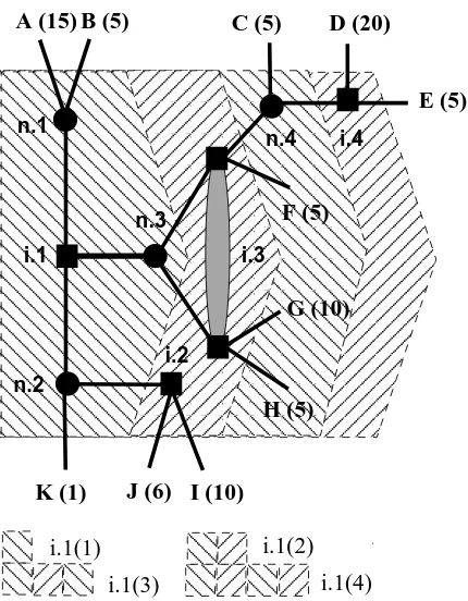
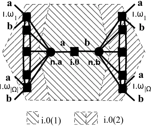
Turning to a more specific description of the model, I consider sequential decision problems of finite length with uncertainty, in their extensive form. The payoffs to terminal nodes and the decision maker’s preferences over these payoffs are given (thus, we know and agree upon what her choices in the given problem should be, if she were fully-rational). For simplicity, the agent is presumed to have expected utility preferences over the terminal payoffs.3 To illustrate, consider the decision problem depicted in Figure 1. Decision and chance nodes are depicted by squares and circles, respectively. The agent’s information seti.3 is a non-singleton (depicted by the shaded oval). The terminal nodes are indexed{A, . . . ,K}while the values in brackets represent the corresponding terminal utility payoffs. The decision maker must choose a plan of action, at her initial node i.1, given a specification f of distributions at each chance node. For example, suppose f assigns probability 1/2 to each branch at n.3 and n.4, and probability 1 to the branches leading to the terminal nodes B and K at n.1 and n.2, respectively. Under unbounded rationality and, thus, perfect foresight, the agent’s plan of action would clearly choose the middle branch at i.1, the upper branch at the information set i.3, and the branches leading to the terminal nodes I and D ati.2 and i.4, respectively. Her expected utility payoff would be 45/4.
In my approach, the search process truncates the decision-tree into horizons, with a horizon of foresight t consisting of all chains of information sets with length at most t. The decision-tree of Figure 2 defines a finite increasing sequence of values for the foresight of search,t∈ {1,2,3,4}, and a corresponding increasing sequence of nested horizons (depicted, in the figure, by combining adjacent hatched regions from left to right). For instance, the horizon of foresight 1 starting ati.1, denoted
i.1(1), is given by the collection {n.1, n.2, n.3}, while the horizon of foresight 2, denoted i.1(2), by i.1(1)∪ {i.2, i.3}. In this example, having foresightt= 4 suffices for rational decision-making. For the horizon i.1(1), the agent knows her utility payoffs at the terminal nodes A,B, and K, as they directly succeed nodes within the horizon. Thus, if Nature’s playf is as above, the agent can correctly assess the payoffs to choosing the upper or the lower branch ati.1; she knows that they are 5 and 1, respectively. In contrast, she cannot necessarily assess correctly her payoff from choosing the middle branch at i.1 since she does not know with certainty the exact terminal consequences of her possible future actions. She assigns, therefore, an expected utility payoff according to some subjective probability distribution over the terminal nodes of the continuation problem (i.e. over
00000000000000
00000000000000
00000000000000
00000000000000
00000000000000
00000000000000
00000000000000
00000000000000
00000000000000
00000000000000
00000000000000
00000000000000
11111111111111
11111111111111
11111111111111
11111111111111
11111111111111
11111111111111
11111111111111
11111111111111
11111111111111
11111111111111
11111111111111
11111111111111
000000000000
000000000000
000000000000
000000000000
000000000000
000000000000
000000000000
000000000000
000000000000
000000000000
000000000000
000000000000
000000000000
111111111111
111111111111
111111111111
111111111111
111111111111
111111111111
111111111111
111111111111
111111111111
111111111111
111111111111
111111111111
111111111111
0000000000
0000000000
0000000000
0000000000
0000000000
0000000000
0000000000
0000000000
0000000000
0000000000
0000000000
0000000000
0000000000
1111111111
1111111111
1111111111
1111111111
1111111111
1111111111
1111111111
1111111111
1111111111
1111111111
1111111111
1111111111
1111111111
0000000
0000000
0000000
0000000
0000000
0000000
0000000
0000000
0000000
0000000
0000000
0000000
0000000
1111111
1111111
1111111
1111111
1111111
1111111
1111111
1111111
1111111
1111111
1111111
1111111
1111111
n.4 i.2 i.400
00
11
11
0
0
1
1
0
0
1
1
0
0
0
1
1
1
00
00
00
11
11
11
00
00
00
11
11
11
00
00
00
11
11
11
00
00
11
11
00
00
11
11
0
0
1
1
i.1 H (5) G (10) E (5) D (20) C (5) B (5) A (15) F (5) n.3 n.1 n.2J (6) I (10) K (1)
i.1(1) i.1(2)
i.1(3) i.1(4)
[image:7.595.199.414.70.346.2]i.3
Figure 1: Foresight and Horizons of Search
the utility payoffs at C,D, . . . ,H). A horizon of longer foresight, such as i.1(2), gives the agent more precise information about some of the consequences of her choices (for example, underi.1(2), she will know her expected payoff from choosing the lower branch at i.3), but could also be more costly to consider.
Suppose that an agent chooses the upper branch ati.1. Such a choice can be rationalized under bounded rationality and limited foresight. The terminal nodes A, B, and K fall within the limits of the horizon i.1(1); even under the most myopic foresight,t= 1, the agent can correctly account for her expected payoff from choosing the upper and lower branches at i.1. With respect to the middle branch, however, she can only have some belief about her continuation payoff. Her observed choice ati.1 (i) reveals that she believes her expected continuation payoff to be less than 5 and (ii) implies that the increase in her complexity costs of extending her foresight from t= 1 to t= 4 is equal to 25/4, the corresponding welfare loss from not doing so.
additional complexity costs in order to extend her foresight from t = 2 to t = 4. Yet, since she intends to choose the upper branch ati.4 with non-zero probability, she is planning to choose the upper branch ati.3. Consequently, her belief about her continuation payoff from the middle branch at i.1 must be at least 15/2. Therefore, the additional search costs to extend her foresight from
t= 2 to t= 4 can be at most 15/4, the implied welfare loss from not doing so.
My approach in modeling bounded rationality fits into a large literature in economics. In most of this literature, however, aspects of the limitations leading to bounded rationality are taken to be exogenously-fixed. MacLeod [51] develops a search cost model, drawing on work in computer and cognitive sciences, in which both the payoffs and the costs of search are taken together to form an exogenously-given net-value function while search proceeds according to a heuristic algorithm (see also Eboli [19]). Models of limited foresight in repeated games (Rubinstein [63]; Jehiel [39], [39], [41],[42]) take the foresight to be exogenously given, implying that the complexity of the stage-game matters equally throughout the repeated stage-game. When the set of contingencies that define the stage-game is not a singleton, however, the number of contingencies within a horizon increases in a combinatorial manner with the number of periods. In contrast, the notion of complexity introduced here incorporates both the number of periods and the number of contingencies within a given period. More importantly, the foresight of search is determined endogenously, which is crucial for explaining behavior in the applications I examine. In the work on repeated games played by finite automata (Neyman [52], [53]; Rubinstein [63], [63]; Abreu and Rubinstein [1], Piccione and Rubinstein [56], Kalai and Stanford [45], Sabourian [65]), the number of states of a machine is often used to measure complexity, leading to a decision-making framework that can be incorporated within my approach (see Section 3.5.3). Another strand of finite automata research focuses on the complexity of response rules (Eliaz [20], Chatterjee and Sabourian [12], Gale and Sabourian [26]).4 While this notion of complexity is more comprehensive than the one presented here, it is unclear how it can be applied beyond repeated games, sequential matching and bargaining.5
The paper is organized as follows. Section 2 presents the general model and the main results. Section 3 develops some further results, including an endogenous stopping rule for search, and discusses the main implications of the analysis as well as some of the related literature in more detail. The applications are examined in Section 4 and Section 5 concludes. Finally, Appendix A offers an index for the notation introduced in Section 2 while Appendix B extends the analysis of Section 4.3 to a more general setting.
4Response complexity compares two response rules that are otherwise identical but for their prescriptions on some
partial history of play. If, for this partial history, one assigns the same action irrespective of the current state of the machine while the other has the action dependent upon the state, the former is regarded as corresponding to lower complexity.
5With respect to machine complexity, response complexity comes closer to a complete ordering: two machines can
2
Modeling Bounded Rationality
A decision problem can be viewed as a game between the agent, who is strategic, and Nature. As a game, it is defined by the set of observable events, the sets of possible plans of action for the agent and Nature, and the agent’s utility payoff function over the terminal contingencies. It can be depicted by a directed graph Γ = ⟨D,A⟩ with D and A being the set of nodes and arcs, respectively. The elements ofA correspond injectively to pairs of nodes (d, d′) such that d, d′ ∈ D
withd̸=d′ and d′ an immediate successor ofdon the graph. Letting Ω denote the set of terminal nodes andHbe the collection of the sets of nodes at which the same player chooses from the same set of actions, Hforms a partition of D \Ω into information sets. H will denote the collection of the information sets where the agent acts. H \H is the collection of Nature’s chance nodes. Let also D(h) denote the collection of nodes comprising the information set h∈ H. I will be referring to h as an immediate successor of some d∈ D, denoted by d◃h, if there existsd′ ∈D(h) that immediately-succeeds d. Similarly, h′ ∈ H withh′̸=h is animmediate successor ofh, denoted by
h◃h′, if there existsd∈D(h) and d′ ∈D(h′) withd◃d′.
2.1 Limited Foresight
When decision-making is constrained by limited foresight, the agent chooses optimally, from her set of strategic alternatives against Nature’s play, taking into account, however, only a subset of the set of possible future contingencies. Specifically, she considers only some part of the decision-tree that lies ahead of her current decision node. Since a pair of plans of action for the agent and Nature defines a sequence of immediately-succeeding information sets that may occur with positive probability, I will restrict attention to parts of the decision-tree consisting of chains of arc-connected information sets. In what follows, I introduce the necessary concepts and notation to describe the precise structure of these parts and, thus, how search is directed through the graph.
For a positive integert, apath from the nodedto the information set h′ of lengthtis a sequence of arc-connected information sets{hτ}tτ=1⊆ H such thatht=h′,d◃h1, and hk◃hk+1
fork∈ {1, ..., t−1}. It will be denoted byd◃{hτ}tτ=1. The union of all paths of length at mostt
that start from somed∈D(h)
h(t) = ∪
d∈D(h)
∪
k∈{1,...,t}
{
d◃{hτ}kτ=1
}
defines thehorizon of foresight t starting at the information set h. This is the collection of all chains of information sets starting ath whose length is at mostt. Thecontinuation problem starting at h, denoted by Γh, is the union of all horizons on the graph starting at h.6 Observe
6This is the standard definition of a continuation problem which is to be distinguished from a subgame: a subgame
that the horizons can be ordered by proper set-inclusion and since
t′ > t ⇐⇒ h(t)⊂h(t′) ∀t, t′ ∈N\ {0}
this ordering can be equivalently represented by the standard ordering on the foresight length. Notice also that, in finite trees, Γh =h(Th) for some positive integer Th.
Let Ωh be the set of terminal nodes that may occur conditional on play having reached some
d∈D(h). If h(t) ⊂Γh, thenh(t) defines a partition of Ωh into the collection of terminal nodes
that are immediate successors of information sets within the horizon and its complement. The collection is given by
Ωh(t) ={y∈Ωh : ∃h′∈h(t)∧d′ ∈D(h′)∧d′◃y}
A terminal node y∈Ωh(t) will be called observable withinh(t).
The set of available actions at each of the nodes in D(h) will be denoted by A(h). A pure strategy is a mapping s : H → ×h∈HA(h) assigning to each of the agent’s information sets an
available action. Let S be the set of such mappings in the game. A mixed strategy for the agent will be denoted by σ ∈ Σ = ∆ (S) . A deterministic play by Nature is a mapping q : H \H → ×d′∈H\HA(d′) assigning to each chance node in H \H a move by Nature. Q is the set of such
mappings in the game andf ∈∆ (Q) denotes a mixed strategy by Nature. Let alsop(d|σ, f) be the probability that the nodedis reached under the scenario (σ, f). Given that play has reachedd, the conditional probability that node d′ will be reached under (σ, f) will be demoted by p(d′|d, σ, f)
withp(d′|d, σ, f) = 0 if d′ cannot follow fromdorp(d|σ, f) = 0,.
The set of terminal nodes that may occur under (σ, f), if play starts at a node of the information set h, is given by
Ωh(σ, f) ={y∈Ωh: ∃d∈D(h)∧p(y|d, σ, f)>0}
Finally,
Ωh(t, σ, f) = Ωh(t)∩Ωh(σ, f)
is the collection of terminal nodes which are observable withinh(t) and may occur under (σ, f) if play starts at a node of h.
2.1.1 An Example
example, suppose thatf assigns probability 1/2 to each branch atn.3 andn.4, and probability 1 to the branches leading to the terminal nodes B and K atn.1 andn.2, respectively. Under unbounded rationality and, thus, perfect foresight, the agent can account for every possible contingency within the continuation problem (the entire tree here). Assuming for simplicity that she has expected utility preferences over final outcomes, her plan of action would choose the middle branch at i.1, the upper branch at the information set i.3, and the branches leading to the terminal nodes I and D at i.2 and i.4, respectively.7
00000000000000
00000000000000
00000000000000
00000000000000
00000000000000
00000000000000
00000000000000
00000000000000
00000000000000
00000000000000
00000000000000
00000000000000
11111111111111
11111111111111
11111111111111
11111111111111
11111111111111
11111111111111
11111111111111
11111111111111
11111111111111
11111111111111
11111111111111
11111111111111
000000000000
000000000000
000000000000
000000000000
000000000000
000000000000
000000000000
000000000000
000000000000
000000000000
000000000000
000000000000
000000000000
111111111111
111111111111
111111111111
111111111111
111111111111
111111111111
111111111111
111111111111
111111111111
111111111111
111111111111
111111111111
111111111111
0000000000
0000000000
0000000000
0000000000
0000000000
0000000000
0000000000
0000000000
0000000000
0000000000
0000000000
0000000000
0000000000
1111111111
1111111111
1111111111
1111111111
1111111111
1111111111
1111111111
1111111111
1111111111
1111111111
1111111111
1111111111
1111111111
0000000
0000000
0000000
0000000
0000000
0000000
0000000
0000000
0000000
0000000
0000000
0000000
0000000
1111111
1111111
1111111
1111111
1111111
1111111
1111111
1111111
1111111
1111111
1111111
1111111
1111111
n.4 i.2 i.400
00
11
11
0
0
1
1
0
0
1
1
0
0
0
1
1
1
00
00
00
11
11
11
00
00
00
11
11
11
00
00
00
11
11
11
00
00
11
11
00
00
11
11
0
0
1
1
i.1 H (5) G (10) E (5) D (20) C (5) B (5) A (15) F (5) n.3 n.1 n.2J (6) I (10) K (1)
i.1(1) i.1(2)
i.1(3) i.1(4)
[image:11.595.198.414.192.468.2]i.3
Figure 2: Foresight and Horizons of Search
Under bounded rationality, the search process is structured in my approach such that it trun-cates the decision-tree into horizons, with a horizon of foresighttconsisting of all chains of informa-tion sets with length at mostt. The decision-tree of Figure 2 defines a finite increasing sequence of values for the foresight of search,t∈ {1,2,3,4}, and a corresponding increasing sequence of nested horizons (depicted, in the figure, by combining adjacent hatched regions from left to right).8 For
t= 1, the search horizon is given byi.1 (1) ={n.1, n.2, n.3}. Fort= 2, there are two chains of infor-mation sets of that length,i.1◃{n.2, i.2}andi.1◃{n.3, i.3}. The collection{n.1, n.2, n.3, i.2, i.3}
defines the horizon i.1 (2). Since only one chain of length t = 3 starts at i.1, i.1 ◃{n.3, i.3, n.4},
7The analysis can accommodate also non-expected utility preferences (see Section 3.2).
8In this framework, with respect to the length of its foresight, the search for the optimal alternative proceeds
the horizon i.1 (3) is given by {n.3, i.3, n.4} ∪i.1 (2). Finally, {n.3, i.3, n.4, i.4} ∪i.1 (3) defines
i.1 (4) (giving the entire tree). The set of terminal nodes that can be reached from i.1 is, of course, Ωi.1 = ∪Kj=A{j}. The sets, though, that are observable within the horizons of search are given,
respectively, by Ωi.1(1) ={A,B,K}, Ωi.1(2) = Ωi.1(1)∪ {F ,G,H,I,J}, Ωi.1(3) = Ωi.1(2)∪ {C}, and
Ωi.1(4) = Ωi.1.
Let σ prescribe positive probabilities for each of the available actions at i.1, i.2, and i.4, but probability 1 to Down at i.3. The sets of terminal nodes that may occur under the scenario (σ, f) and are observable within the horizons of search are given by Ωi.1(1, σ, f) = {B,K} and
Ωi.1(t, σ, f) ={F,H,B,K}= Ωi.1(σ, f) fort≥2. If s∈support{σ} is the pure strategy that plays
the middle branch at i.1, then Ωi.1(1, s, f) =∅while Ωi.1(t, s, f) ={F,H}= Ωi.1(s, f) for t≥2.
Similarly, for the decision to be made at the information seti.3, we have Ωi.3(1) ={C,F,G,H},
Ωi.3={C,D,E,F,G,H}= Ωi.3(2), and Ωi.3(1, σ, f) ={F,H}= Ωi.3(σ, f).
2.2 Behavior under Limited Foresight
Starting at h ∈H, the agent may consider a horizonh(t) ⊆Γh instead of the entire continuation
problem. Given its limited foresight, her decision-making is sophisticated: with respect to the terminal nodes that are observable under her current foresight, she can correctly optimize according to her underlying preferences over terminal consequences. Regarding outcomes beyond her horizon, she is not able to do so, even though she is aware that there may exist contingencies which could occur, under Nature’s f ∈ ∆ (Q) and her choice σ ∈ Σ, but are currently unforeseen within
h(t). I will assume that the agent evaluates the set of possible but currently unforeseen terminal contingencies according to the expectation operatorEµ, for some probability distributionµon this
set.
Formally, let u: Ω→R++ represent the agent’s preferences over terminal outcomes.9 Abusing
notation slightly, for any setY of terminal nodes, let
u(Y) =∑
y∈Y
u(y) and u(∅) = 0
Given a pure strategy profile (s, q)∈S×Q,u(Ωh(s, q)) is the agent’s total utility payoff from the
continuation problem Γh. Preferences over lotteries on terminal consequences admit an expected
utility representation. The agent’s expected utility payoff under (σ, f)∈Σ×∆ (Q), given that play reached h, is given, therefore, by
uh(σ, f) =
∑
s∈S
∑
q∈Q
σ(s)f(q)u(Ωh(s, q))
9Although at no loss of generality, the non-negativity of the terminal utility payoffs is essential for determining
while
Rh(f) = arg max
σ∈Σ uh(σ, f)
is the set of best-responses under rational decision-making (unlimited foresight).
Under limited foresight, the notation must be enriched to distinguish the payoffs associated with terminal nodes that are observable within the horizon from those corresponding to terminal nodes beyond. Since the agent perceives correctly the former collection, the payoff from (s, q) at terminal nodes that are observable under foresight t is given by u(Ωh(t, s, q)). Within the
unobservable set Ωh\Ωh(t), however, the terminal contingencies can be reached via any strategy
profile (σ′, f′) ∈ Σ×∆ (Q) that results in the same play as (s, q) within h(t). That is, (σ′, f′) is another possible continuation scenario from the perspective of the horizon h(t). By Kuhn’s Theorem, we can define the following concept:
Definition 1 Let h ∈ H and h(t) ⊆ Γh. Two strategy profiles (σ, f),(σ′, f′) ∈ Σ×∆ (Q) are
h(t)-equivalent, denoted by(σ, f) ≃
h(t)(σ
′, f′), if both prescribe the same probability distribution at
each node in D(eh), for any information set eh∈h(t). That is,
(σ, f) ≃
h(t)
(
σ′, f′) iff (σ, f)|h(t)≡(σ′, f′)|h(t)
Here, (σ,e fe)|h(t) denotes the restriction to h(t) of the unique behavior-strategy profile that corre-sponds to (σ,e fe).
Regarding outcomes beyond the truncated tree, the set of terminal nodes that may follow from any d∈D(h) when (s, f) is played withinh(t) is given by10
Ωh(t, s, f) =
∪
(s′,f′)∈S×∆(Q):(s′,f′)≃
h(t)(s,f)
Ωh
(
s′, f′)\Ωh(t, s, f)
The set of the corresponding terminal utility payoffs will be denoted by
Uh(t, s, f) =
{
u(y) :y∈Ωh(t, s, f)
}
⊂R++
The agent evaluates the set Ωh(t|s, f) of possible but currently unforeseen terminal contingencies
according to the expectation operatorEµ[Uh(t, s, f)] for some probability measureµon Ωh(t|s, f).
Observe that, letting infUh(t, s, f) and supUh(t, s, f) denote the minimum and maximum of this
set, respectively, this criterion can be represented as
Eµ[Uh(t, s, f)] =αh(t, s, f) infUh(t, s, f) (1)
for some αh(t, s, f) ∈
[
1,supUh(t,s,f) infUh(t,s,f)
]
. In Section 3, I discuss the robustness of my results with respect to using the this particular representation. The total expected utility payoff under horizon
10Observe that Ω
h(t), when (σ, f) is played within the horizon, is given by the mapping Uh(·) : {1, ..., Th} ×Σ×
∆ (Q)→R++ with
Uh(t, σ, f) = u(Ωh(t, σ, f)) +
∑
s∈S
σ(s)Eµ[Uh(t, s, f)] (2)
= u(Ωh(t, σ, f)) +
∑
s∈S
σ(s)αh(t, s, f) infUh(t, s, f)
The second term above corresponds to the agent’s expected utility payoff from the possible but currently unforeseen future terminal contingencies when (σ, f) is played within h(t). It will be called, henceforth, thecontinuation valueof the horizonh(t) under (σ, f).
A binary relation can now be defined on {1, ..., Th} by
t%h t′ iff max
σ∈Σ Uh(t, σ, f)≥maxσ∈ΣUh
(
t′, σ, f)
This is the agent’s preference relation over the horizons in Γh when Nature’s strategy is f. By
construction, it admits the utility representation
Vh(t, f) = max
σ∈Σ Uh(t, σ, f)
while the correspondence
Rh(t, f) = arg max
σ∈Σ Uh(t, σ, f)
gives the optimal choices from Σ against f under the horizon h(t). The optimization problem maxt∈{1,...,Th}Vh(t|f) determines optimal horizon - strategy set pairs{h(t
∗), R
h(t∗, f)} ∈Γh×Σ.
2.3 Bounded Rationality
The behavior under limited foresight described above can be used to compare boundedly-rational with rational decision-making once some minimal structure is imposed on the underlying choice rules.
Definition 2 A choice rule Ch(S, f) ⊆ Σ, against f ∈ ∆ (Q) at h, is admissible if there exists
t∈ {1, ..., Th} such that Ch(S, f)≡Rh(t, f).
The criterion in Definition 2 admits really any reasonable choice. It refuses only choice rules which ignore strict dominance to an extent that it is impossible to draw a line between bounded rationality and irrationality. To see this, let s⋆ ∈ C
h(S, f) for some inadmissible Ch(S, f). By
definition, we cannot find any t ∈ {1, ..., Th} and an corresponding array [αh(t, s, f)]s∈S such
that Uh(t, s, f) ≤ Uh(t, s∗, f) for all s ∈ S. Fixing t ∈ {1, ..., Th}, this implies the existence
of some es ∈ S such that Uh(t,es, f) > Uh(t, s∗, f) for any αh(t,s, fe ) ∈
[
1,supUh(t,es,f) infUh(t,es,f)
]
αh(t, s∗, f) ∈
[
1,supUh(t,s∗,f) infUh(t,s∗,f)
]
. Taking αh(t,es, f) = 1 and αh(t, s∗, f) = supUh(t,s
∗,f)
infUh(t,s∗,f), by (1) and
(2), we get
min
(s′,f′)∈S×∆(Q): (s′,f′)≃
h(t)(es,f) uh
( s′, f′)
= u(Ωh(t,es, f)) + min
(s′,f′)∈S×∆(Q): (s′,f′)≃
h(t)(es,f) {
uh(s′, f′)−u(Ωh(t,es, f))}
> u(Ωh(t, s∗, f)) + max (s′,f′)∈S×∆(Q): (s′,f′)≃
h(t)(s ∗,f)
{ uh
(
s′, f′)−u(Ωh(t, s∗, f))
}
= max
(s′,f′)∈S×∆(Q): (s′,f′)≃
h(t)(s ∗,f)uh
( s′, f′)
That is, an inadmissible choice rule opts for the plan of action s∗ against f even though there exists a planesunder which the worst possible outcome, from the perspective of the horizonh(t), is strictly better than the best possible outcome under s∗. Moreover, since the foresighttwas taken arbitrarily, this applies even for every horizon in Γh.
The notion of admissibility of Definition 2 imposes some very weak restrictions on the extent to which the choice behavior under study departs from rationality. I will now demonstrate that, within the realm of admissibility, the behavior under limited foresight in 2 can be used as a platform onto which both rational as well as boundedly-rational decision-making can be represented. For this, I must make the following behavioral assumption.
A.1 ∀h∈H and ∀(s, f)∈S×∆ (Q) αh(t, s, f) is non-decreasing on {1, ..., Th}
Recall that the mappingαh(t, s, f) depicts the agent’s belief about the continuation value of the
horizonh(t) under the profile (s, f) as a combination between the best and worst utility payoff out of the set of currently unforeseen but possible future terminal contingencies when (s, f) is played within h(t). The assumption amounts simply to requiring that the agent does not become more pessimistic about the continuation value of her horizon of search, with respect to a given profile (s, f), as her search deepens. This suffices for the agent to be exhibiting a weak preference for deepening her horizons of search.
Proposition 1 Under Assumption A.1, the relation %h exhibits a weak preference for larger
hori-zons:
t > t′ =⇒ t%h t′
Notice that a weak preference for deeper search can be equivalently expressed as ∆tVh(t, f) ≥ 0
∀t∈ {1, ..., Th}. Therefore,
max
t∈ThVh(t, f) =Vh(Th, f) = maxσ∈Σuh(σ, f)
At any h ∈ H, an agent with preferences %h on {1, ..., Th} will choose the maximal horizon and,
Under assumption A.1, the suggested behavior under limited foresight is indistinguishable from rationality. It can be taken, therefore, as a benchmark: departures from rational decision-making can be equivalently depicted as departures from this behavior under limited foresight. Within the context of admissible choice rules, I will restrict attention to departures that result in a welfare loss relative to rational decision-making.
Definition 3 An admissible choice rule Ch(S, f) is boundedly-rational if Ch(S, f) ≡Rh(t∗, f)
and Vh(t∗, f)< Vh(Th, f), for some t∗ ∈ {1, ..., Th−1}.
Since it is admissible, a boundedly-rational choice rule should give a best-response set that is optimal for the optimization over Th of some appropriate transformation of the value function
Vh(t, f). This transformation could represent a variety of psychological, behavioral, cognitive or
ability factors that force departures from rationality. However, boundedly-rational choices ought to be admissible with respect to every foresightt∈ {1, ..., Th}. Moreover, preferences over lotteries
on the set of terminal consequences should admit an expected utility representation. Clearly, we must restrict attention to strictly-increasing, affine transformations of Uh(t,·, f). Let, therefore,
e
Uh :{1, ..., Th} ×Σ×∆ (Q)→R++ be defined by
e
Uh(t, σ, f) =γh(t, f)Uh(t, σ, f) +γh0(t, f)
for some functions γh :Th×∆ (Q)→R++ andγ0h :Th×∆ (Q)→R. The optimization problem
now becomes
max
t∈{1,...,Th}
γh(t, f)Vh(t, f) +γh0(t, f) (3)
Let th(f) denote the smallest optimal foresight in (3). The corresponding set of maximizers from
Σ will be called the boundedly-rational best-response set, denoted by BRh(f).
The formulation in (3) embeds rational decision-making as a special case. More importantly, it does so in a way that establishes the functions γh and γh0 as indicators of bounded rationality.
For the agent to be boundedly-rational against f at h, at least one of two functions must not be constant on the set{th(f), ..., Th}. Put differently, rational decision-making againstany f ∈∆ (Q)
ath is consistent only with both functions being constant on {minf∈∆(Q)th(f), ..., Th
}
×∆ (Q). Proposition 2 Let f ∈∆ (Q). The following are equivalent:
(i) The optimization in (3) represents %h on the set {t(f), ..., Th}
(ii) The functions γh and γh0 are constant on the set {t(f), ..., Th}.
For the remaining of the paper, I will normalizeγ0
hto be the zero function on{1, ..., Th}×∆ (Q).
This allows for an empirically testable and robust relation between the terminal utility payoffs of the decision problem at hand and the agent’s optimal horizon. To see this, observe first that
∆t[γh(t, f)Vh(t, f)] = γh(t+ 1, f)Vh(t+ 1, f)−γh(t, f)Vh(t, f)
while, at the optimal foresight, we must have ∆t[γh(t(f), f)Vh(t(f), f)]≤0. Since ∆tVh(t, f)≥
0 on{1, ..., Th}(recall Proposition 1),
Remark 1 For the representation in (3), let γ0
h be the zero function on {1, ..., Th} ×∆ (Q). Then,
∆tγh(t(f), f)≤0.
Moreover, all utility payoffs of terminal outcomes are strictly positive (i.e. Vh(t, f) > 0 for all
(t, f)∈Th×∆ (Q), h∈H) and so is the function γh. Clearly, we must have
∆tVh(t(f), f)
Vh(t(f), f)
≤ −∆tγh(t(f), f)
γh(t(f) + 1, f)
Since the transformation function γh does not vary with the terminal utility payoffs, the validity
of the above inequality is completely determined by the left-hand side quantity. If this increases sufficiently, other things remaining unchanged, the inequality will no longer be valid.11 Similarly, by the optimality of (f), we have ∆t[γh((f)−1, f)Vh((f)−1, f)]≥0 and, thus,
∆tVh((f)−1, f)
Vh((f)−1, f)
≥ −∆tγh((f)−1, f)
γh((f), f)
If the quantity ∆tVh((f)−1,f)
Vh((f)−1,f) decreases sufficiently, ceteris paribus, the inequality will cease to hold. 12
Remark 2 In the representation in (3), letγh0 be the zero function on{1, ..., Th} ×∆ (Q). Suppose
that the specification of the terminal utility payoffs in ∪s∈SΩh(s, f) changes and denote by told(f)
and tnew(f) the optimal horizons under the original and new specifications, respectively. Let also
Vnew
h (t, f) denote the value function in (3) under the new specification. Then,
1. tnew(f) =told(f) if the changes in the terminal utility payoffs are such that
∆tVhnew(told(f), f)
Vnew
h (told(f), f)
∈
[
0,−∆tγh
(
told(f), f)
γh(told(f), f)
] and
∆tVhnew(told(f)−1, f)
Vnew
h (told(f)−1, f)
∈
[
−∆tγh
(
told(f), f)
γh(told(f), f)
,+∞
)
(2.i) tnew(f)> told(f) if the changes in the terminal utility payoffs are such that
∆tVhnew
(
told(f), f)
Vnew
h (told(f), f)
/
∈
[
0,−∆tγh
(
told(f), f)
γh(told(f), f)
] and
∆tVhnew
(
told(f)−1, f) Vnew
h (told(f)−1, f)
∈
[
−∆tγh
(
told(f), f) γh(told(f), f)
,+∞
)
11Other things remaining unchanged refers here to the quantities ∆tVh(t,f)
Vh(t,f) , fort∈ {1, ..., Th} \ {t(f)}. 12Ceteris paribusrefers to the quantities ∆tVh(t,f)
(2.ii) tnew(f)< told(f) if the changes in the terminal utility payoffs are such that
∆tVhnew
(
told(f), f)
Vnew
h (told(f), f)
∈
[
0,−∆tγh
(
told(f), f)
γh(told(f), f)
] and
∆tVhnew
(
told(f)−1, f) Vnew
h (told(f)−1, f)
/
∈
[
−∆tγh
(
told(f), f) γh(told(f), f)
,+∞
)
The suggested normalization guarantees also that the optimal horizon againstf ∈∆ (Q) at h∈H
in (3) is not affected by affine transformations in the utility representation of the agent’s preferences over terminal consequences.
Claim 1 For the representation in (3), let γ0
h be the zero function on {1, ..., Th} × ∆ (Q) and
consider an affine transformation, λu(·) with λ > 0, of the utility representation of preferences over the terminal consequences. Then, told(f) =tnew(f).
2.4 Complexity and its Costs
In general, different search horizonsh(t)∈Γh impose different degrees of informational limitations
on the agent’s decision-making. The particular search horizon the agent considers should, therefore, matters for her response against anyf ∈∆ (Q). Yet, the proof of Proposition 1 shows that this is not always the case since the preference for larger horizons is not necessarily strict. Depending on the structure of the problem and Nature’s play, the marginal benefit from deeper search, ∆tVh(t, f),
may be zero. In such a case, extending the search horizon fromh(t) toh(t+ 1) does not affect the set of optimal responses againstf. This corresponds to a non-complex decision-making situation.
Definition 4 For any h ∈ H and t ∈ {1, ..., Th−1}, we say that f ∈∆ (Q) is h(t)-complex if
∆tVh(t, f)>0. f is h-complexif it is h()-complex for somet∈ {1, ..., Th}. The decision problem
is complex ath, if there exists f ∈∆ (Q) that is h-complex.
Example 2.4: For the decision problem of Figure 2, suppose that Nature may move in either direction atn.3 andn.4 with equal probability, left at n.1 with any probability p, and determinis-tically down at n.2. At i.1, if the agent chooses the upper branch, she expects a utility payoff of 5 + 10p. If she chooses the lower branch, her payoff will be 1. The middle branch corresponds to a continuation value of 5αi.1(1, m, f) fort= 1 (the worst case scenario is her moving Down at i.3),
10
2 +52αi.1(2, m, f) fort= 2, 102 +54+54αi.1(3, m, f) fort= 3 (fort∈ {2,3}, the worst case scenario
entails moving Up at i.3 but Down ati.4), and 454 fort= 4. Notice that αi.1(1, m, f)∈
[
1, 102+ 20
2
5
]
whereas αi.1(2, m, f), αi.1(3, m, f)∈[1,205].
Ifp≥ 58, the expected value of every horizon is 5 + 10p; Nature’s play is not complex ati.1. For
fort= 2, 5 + 5 max{2p,14 +14αi.1(3, m, f)}fort= 3, and 454 for t= 4. Nature’s play can now be
complex ati.1 (for instance, let p < 14).
Consider now the function Ch:{1, ..., Th} →R defined by
Ch(t, f) = [1−γh(t, f)]Vh(t, f)
This function acquires some interesting properties when the notion of complexity defined above is linked with the representation in (3). Sinceth(f) denotes an optimal horizon in (3), we have
Vh(th(f), f)−Ch(th(f), f) ≥ Vh(t, f)−Ch(t, f) =⇒
Ch(t, f)−Ch(th(f), f) ≥ Vh(t, f)−Vh(th(f), f)
≥ 0 (by Proposition 1) ∀t∈ {t(f), ..., Th}
If we normalize γh(th(f), f) = 1, then Ch(th(f), f) = 0. Since now Ch(t, f) ≥ 0, for any
t ∈ {t(t)Th} and f ∈ ∆ (Q), the function Ch becomes a cost function on {t(f), ..., Th}. If,
moreover, we restrict gh to take values in the set (0,1], Ch becomes a cost function on the entire
set {1, ..., Th}. In either case, it will be called, henceforth, thecomplexity cost function.
By the very definition of the complexity-cost function, whenγh0is the zero function on{1, ..., Th},
the decision-making under bounded rationality given in (3) admits equivalently the following rep-resentation
max
t∈{1,...,Th}
Vh(t, f)−Ch(t, f) (5)
This representation illustrates the economic meaning of the complexity costs. Notice that, if ∆tCh(t, f) = 0 for all t∈ {1, ..., Th}, the representation is equivalent to rational decision-making.
The functionCh(·, f) depicts, therefore, the discrepancy between the payoff,γh(t, f)Vh(t, f), that
the boundedly-rational agent assigns to her best response, Rh(t, f), against f when her horizon is
limited to h(t) and the actual payoff, Vh(t, f), from Rh(t, f) against f when the foresight is
re-stricted tot. It is trivial to verify the following relations between the marginal benefits of extending search around the optimal foresight againstf and the corresponding marginal complexity costs. In Section 3.4, I show that they lead to important testable implications of my model.
Remark 3 For the representation in (3), let g0h be the zero function on {1, ..., Th}. For any f ∈
∆ (Q) and h∈H, we have
∆tCh(t(f), f)≥∆tVh(t(f), f) and ∆tCh(t(f)−1, f)≤∆tVh(t(f)−1, f)
Claim 2 For the representation in (3), let γ0
h be the zero function on {1, ..., Th}. If f ∈∆ (Q) is
not h(t)-complex, then it cannot entail any marginal complexity costs on the horizon h(t). That is,
∆tVh(t, f) = 0 =⇒∆tCh(t, f) = 0
The complexity-cost function affects choices only in complex problems and only where the agent would strictly prefer to expand her horizon if she were not constrained by her bounded rationality. In this sense, the function depicts the presence of (and only of) bounded rationality. To see this, consider again Nature’s mixed strategy in Example 2.4 with p ≥ 58. An agent who chooses the upper branch ati.1 may or may not be boundedly-rational. Such a stochastic play by Nature is not complex enough to reveal bounded rationality from observed choices in this problem. Accordingly, expanding the agent’s foresight does not entail any marginal complexity costs.
Complexity has been defined here with respect to the structure of the decision problem. It depends, therefore, upon the particular conjecture f about Nature’s play. This dependence is reflected in the functionChallowing the model to exhibit an important endogenous form of bounded
rationality. When playing a complex game against a strategic opponent, the perceived ability of the opponent seems to obviously matter when the agent decides how deeply into the game-tree to plan for. Even though Nature is not a strategic player, there is an analogue of this intuition in a decision-theoretic setting. Different conjectures about Nature’s play correspond to different sets of unforeseen contingencies that may occur beyond the current horizon. Hence, the difficulty of a given decision problem varies with the set of Nature’s stochastic plays that the agent considers. In this model, the conjectures about Nature’s play matter not only through the expected terminal payoffs but also directly through the complexity-cost function. This may lead a boundedly-rational agent to choose different horizons in response to different conjectures.
Allowing the complexity costs function to vary on ∆ (Q) offers also a built-in flexibility to differentiate between the length and breadth of a horizon, in terms of complexity. The cost of considering a horizon h(t) against a strictly-mixed f may well be strictly higher than the corre-sponding cost against any pure strategy in the support of f. This could reflect the larger number of contingencies which may happen within the horizon against the mixture. While the foresight ist
in either case, responding againstf requires accounting for more contingencies. Finally, the model allows the functionCh to vary across the information setsh∈H at which decisions are to be made
against f. It can accommodate, therefore, decision-making situations where the complexity of the continuation problem varies at different stages of the problem.
3
Discussion and Related Literature
rationality admits the following representation
max
t∈ThVh(t, f)−Ch(t, f) (6)
In this section, I discuss some of the strengths and limitations of this representation and how it relates to some of the literature.
3.1 Strictly Dominated Strategies Matter
Decision-making under limited foresight is based upon comparing plans of action that lead to terminal outcomes occurring within the agent’s current foresight against her beliefs about the continuation value of plans that do not. Such decision-making is affected by strictly dominated strategies, if the agent’s foresight is not long enough to reveal the dominance.
In finite, non-repeated problems, any (s, q) ∈ S×Q will eventually reach a unique terminal node. That is, one of the two terms of the partition Ωh(t, s, q)∪Ωh(t, s, q) is the empty set, for
any t∈Th, h∈H. There exists, therefore, th(s, q)∈Th such that Ueh(th(s, q), s, q) =u(h, s, q).
Suppose now that es ∈ S does strictly worse than s against q conditional on play having reached
h: u(h, s, q) > u(h,es, q). The presence of sedoes not matter for the objective in (3) as long as
t ≥ th(s, q). For t ≥ maxq∈Qth(s, q), this is true for any strictly dominated strategy es. For
finitely-repeated problems, this argument suggests that the presence of esdoes not matter for the optimization in (3), if there existss∈Sthat does strictly better thanseagainstq in the stage game and the agent’s foresight suffices to cover the stage game.
To illustrate, consider removing the option of moving Down ati.3 in Figure 2. Any strategy that uses this action with positive probability is strictly dominated by any other that assigns probability 1 to Up ati.3. The deletion will not affect the valuationVi.1(t, f), fort≥2, because the dominance
is revealed within the horizon. This is not true, however, fort= 1. Consider the playf of Example 2.4. The continuation value of the middle branch ati.1 is now the one corresponding to the horizon
i.1 (2) in that example, 102 +52αi.1(2, m, f). For αi.1(2, m, f) > 4p, an agent with foresight t= 1
will choose Middle ati.1. This inequality can be satisfied even forp≥ 58; that is, in cases where the agent would choose Up in Example 2.4. The removal of a strictly-dominated option at i.3 makes her here ex-ante, strictly better-off ati.1.
It is equally straightforward to construct a strictly dominated strategy whose introduction makes a boundedly-rational decision maker better off. Following Nature moving left at n.1 in Figure 2, suppose that the agent can now choose between two moves, say Left and Right, for a utility payoff of 15 and 1, respectively. The new problem is equivalent to the old for a rational agent. Yet, for Nature’sfas above, the continuation payoff of choosing Up ati.1, fort= 1, becomes
pαi.1(1, u, f) + 5 (1−p), where αi.1(1, u, f)∈[1,15]. For αi.1(1, u, f)<5, an agent with foresight
Notice that the dependence on strictly dominated strategies obtains only as long as the con-tinuation value of the horizon depends on the length of foresight. The concon-tinuation value of any (s, f) ∈ S×∆ (Q) does not vary with t if and only if αh(t, s, f) = supinfUUh(t,s,f)
h(t,s,f), for all t ∈ Th. If
the agent correctly identifies the best possible future outcome of (s, f) under any horizonh(t), her limited foresight poses no informational limitation for decision-making. She will always choose the same best-response set as if her foresight were unlimited. Planning for future contingencies that lie beyond even the shortest horizon,h(1), is not necessary.
3.2 Robustness
The complexity cost approach is based on measuring the extent of bounded rationality via the implied welfare loss when observed choices differ from those prescribed under rational decision-making. This framework for modeling endogenous bounded rationality is robust to many different ways of evaluating a given (s, f) with respect to the horizon h(t) : t ∈ Th. Specifically, it can
accommodate any functional Uh(t, s, f). A different valuation criterion would define a new value
functionVh(t, f) which, in turn, require a new transformationVeh(t, f) to represent the discrepancies
between Vh(t, f) : t < Th and the criterion of rational decision-making, V (Th, f). Nevertheless,
this representation of endogenous bounded rationality can still be given as the trade-off between
Vh(t, f) and the costs of complexity,Ch(t, f) =Vh(t, f)−Veh(t, f).
The functional defined in (2) is based upon an intuitive interpretation of limited foresight. Namely, that it imposes informational and/or other decision-making constraints only with respect to contingencies that may occur beyond the reach of the current horizon. An obvious way to evaluate the set of such contingencies is via the expectation operator on the set of the corresponding terminal utility payoffs according to some subjective probability distribution the decision maker places on this set. This valuation criterion produces a ranking of the available plans of action that is independent of affine transformations of the utility representation of the preferences over terminal consequences. If we restrict attention, moreover, to strictly positive utility payoffs, it can be equivalently given by the second term on the right-hand side of (2).
Assumption A.1 ensures that the value function Vh(t, f) is non-decreasing in t, for any f ∈
∆ (Q). This monotonicity is crucial for an important feature of my approach to modeling bounded rationality. By specifying precisely how rational decision-making corresponds to a limiting case of the representation, the property provides the necessary structure for the optimal horizon to be obtained endogenously and for the implied complexity costs to be inferred from observed choices. The assumption is restrictive in the following sense. As the foresighttincreases, the agent becomes better-informed about the possible paths of play under (s, f) and drops plans f′ ̸= f such that (s, f′) is h(τ)-equivalent to (s, f) for someτ < t but not for τ =t. Assumption A.1 requires that
αh(·, s, f) is non-decreasing even whenu(h, s, f′)> u(h, s, f).
require-ment, on the consistency of her forecasts about Nature’s play. Specifically, suppose that the agent’s forecast is always correct; that is, it is correct from the perspective of every horizon in Γh. The set
Uh(t, s, f) of terminal utility payoffs that can realize beyond the horizon h(t) under (s, f) is now
given by
Uh(t, s, f)≡
{
x=u(h, s′, f)−u(Ωh(t, s′, f)): s′ ∈S,(s′, f) ≃ h(t)(s, f)
}
⊂R++
As the foresight t∈Th increases, {Uh(t, s, f)}t∈Th forms a decreasing nested sequence. Since the
agent optimizes overS, Assumption A.1 requires now merely that the agent does not become more pessimistic about her abilities to respond optimally against f as her foresight increases.
In general, mins′∈S:(s′,f)≃
h(t)(s,f)
u(h, s, f) is non-decreasing it the foresight t (recall relation
(i) in the proof of Lemma 1). Under the consistency requirement of the preceding paragraph, maxs′∈S:(s′,f)≃
h(t)(s,f)
u(h, s, f) is non-increasing in t. This enables my approach to model also
deci-sion makers whose limited foresight changes along the decideci-sion-tree in a way that may not agree with the sequence {h(t)}t∈Th. Optimizing under horizon h(t) requires that the agent considers
all contingencies in the t-length chains of information sets for all profiles (s, f) : s∈ S. Consider, however, an agent who examines the contingencies, that may occur against f, when she follows the plans s and s∗ along chains of information sets of length t and t∗ > t, respectively. If she prefers s to s∗, we can model her choice by choosing appropriate values for αh(·, f) such that
Uh(t, s, f) ≥ Uh(t, s∗, f). If she chooses s∗ over s, we can construct the valuation criterion such
that Uh(t∗, s, f)≤Uh(t∗, s∗, f). It is easy to check that, for none of the two inequalities above to
be valid, the following two conditions must hold simultaneously:
(i) maxs′∈S:(s′,f)≃
h(t)(s,f)
u(h, s, f)<mins′∈S:(s′,f)≃
h(t)(s
∗,f)u(h, s∗, f)
(ii) mins′∈S:(s′,f) ≃
h(t∗)(s,f)
u(h, s, f)>maxs′∈S:(s′,f) ≃
h(t∗)(s
∗,f)u(h, s∗, f)
But this cannot be since (i) leads to a contradiction of (ii):
min
s′∈S:(s′,f) ≃
h(t∗)(s,f)
u(h, s, f)
≤ max
s′∈S:(s′,f) ≃
h(t∗)(s,f)
u(h, s, f)
≤ max
s′∈S:(s′,f)≃
h(t)(s,f)
u(h, s, f)(i)< min
s′∈S:(s′,f)≃
h(t)(s
∗,f)u(h, s
∗, f)≤ min
s′∈S:(s′,f) ≃
h(t∗)(s
∗,f)u(h, s
∗, f)
≤ max
s′∈S:(s′,f) ≃
h(t∗)(s
∗,f)u(h, s
∗, f)
By choosing the appropriate foresight and values forαh(·, f), the agent’s actual ranking ofsands∗
000000000000
000000000000
000000000000
000000000000
000000000000
000000000000
000000000000
000000000000
000000000000
000000000000
111111111111
111111111111
111111111111
111111111111
111111111111
111111111111
111111111111
111111111111
111111111111
111111111111
000000000
000000000
000000000
000000000
000000000
000000000
000000000
000000000
000000000
000000000
111111111
111111111
111111111
111111111
111111111
111111111
111111111
111111111
111111111
111111111
000000
000000
000000
000000
000000
000000
000000
000000
000000
000000
111111
111111
111111
111111
111111
111111
111111
111111
111111
111111
n.2 n.30
0
0
1
1
1
00
00
11
11
0
0
1
1
0
0
1
1
00
00
11
11
(10) (2) (0) (20) i.1 n.10
0
1
1
i.2 i.3 (3) [image:24.595.220.396.72.243.2]i.1(1) i.1(2) i.1(3)
Figure 3: A Non-Complex Problem
presented here even though the true underlying decision-making criterion might not examine the same length of chains of information sets across all available plans of action.
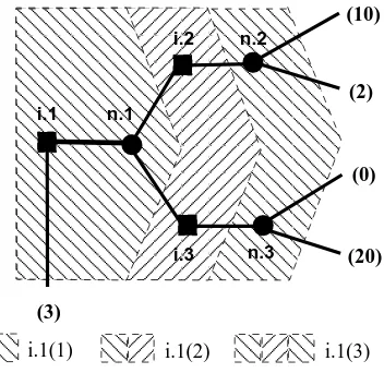
Consistent forecasts provide my approach with another desirable feature. Lemma 2 dictates now that any contingency which lies beyond the current horizon and does not require strategic decisions by the agent cannot add to the current complexity costs. The following example illustrates two immediate implications of this result. First, the benefits and costs of further search are zero along dimensions where further search is futile. Second, calculating expectations with respect to Nature’s probability distributions is not costly; it cannot account for departures from rationality. Discrepancies from rational decision-making can result only from the the agent’s limited ability to handle the complexity of making optimal decisions.
Example 3.2: For the problem of Figure 3, consider the stochastic play f by Nature that places equal probability at the branches of every chance node. There are infinitely many plays,
f′ ̸=f, such that (s, f) and (s, f′) are i.1 (2)-equivalent to f, for anys∈ S. If the setU
h(t, s, f)
of terminal utility payoffs beyond the horizon is defined as in Section 2.2, the agent’s continuation value, for t ≤ 2, depends on her conjecture about the likelihood of the plays f′. As long as the
agent believes that such an f′ is played with non-zero probability, ∆tVi.1(t, f)̸= 0 for t≤2.
Let now Uh(t, s, f) be defined as above. Since the agent has only one available move at i.2
and i.3, the problem is not complex at any of her decision nodes. The value of i.1 (1) is 8 (playing down at i.1 terminates the game within the reach of the horizon for a utility payoff of 3; playing right corresponds to an expected continuation payoff of 8). The best response and the value of the horizoni.1 (t) remain unchanged fort≥2: ∆tVi.1(t, f) = 0 and, thus, ∆tCi.1(t, f) = 0. Notice that