Improving the Length of Con…dence Sets for the Date of a Break in
Level and Trend when the Order of Integration is Unknown
David I. Harvey and Stephen J. Leybourne School of Economics, University of Nottingham
May 2016
Abstract
Harvey and Leybourne (2015) construct con…dence sets for the timing of a break in level and/or trend, based on inverting sequences of test statistics for a break at all possible dates. These are valid, in the sense of yielding correct asymptotic coverage, forI(0)or I(1) errors. In constructing the tests, location-dependent weights are chosen for values of the break magnitude parameter such that each test conveniently has the same limit null distribution. By not imposing such a scheme, we show that it is generally possible to signi…cantly shorten the length of the con…dence sets, whilst maintaining accurate coverage properties.
Keywords: Level break; Trend break; Stationary; Unit root; Con…dence sets. JEL Classi…cation: C22.
1
Introduction
Harvey and Leybourne (2015) [HL] propose methods for constructing con…dence sets for the date of a break in level and/or trend that are robust to both I(0) and I(1) errors. These are based on the approach of Elliott and Müller (2007) [EM] which involves inverting a sequence of tests for a break at all possible dates. HL derive locally best invariant [LBI] tests separately for when the model errors are I(0) and I(1), with resulting con…dence sets providing correct asymptotic coverage regardless of the magnitude of the break. They then suggest using a unit root pre-test procedure to select between theI(0)- andI(1)-based con…dence sets.
The individual test statistics considered by HL are constructed to maximize an average power criterion, subject to a chosen probability measure for the break magnitude at each date. Following EM, HL use a probability measure that, while not indefensible, is essentially chosen for its expediency, in that under the null of a correct break date, each of the statistics has the same limit null distribution, so that the same asymptotic critical value applies for every assumed break location. Kurozumi and Yamamoto (2015) [KY], in the context of an I(0) model similar to that considered by EM where a break occurs in the coe¢ cients on stationary regressors, argue that this is unnatural in that such a weighting scheme is not motivated by power considerations. Moreover, the EM probability measure for the break magnitude implicitly attributes di¤erent weights to breaks occurring at di¤erent timings. KY adopt a more natural probability measure that does not enforce such an arti…cial structure on the testing problem, and …nd that this can deliver power gains relative to the EM approach, which translates into a reduction in con…dence set length. The HL method for constructing con…dence sets for the date of a break in level and/or trend in the presence ofI(1)errors relies on …rst di¤erencing, and bears a close resemblance to the EM and KY model framework. It would be expected, therefore,
that use of a KY-type probability measure might result in increased test power and shorter con…dence sets, at least in the I(1) context. In this paper, we pursue such a modi…cation of HL. The new weighting scheme results in new limit distributions for both theI(0)- andI(1)-based tests, and hence new critical values, which are now location dependent. Using …nite sample Monte Carlo simulations, we then show that this new weighting scheme, while having little e¤ect on coverage rates, can yield a signi…cant shortening of the con…dence intervals, particularly when the errors are I(1), or areI(0)
but exhibit a reasonable degree of persistence.
2
The model and con…dence sets
As in HL we consider a model foryt that permits a level and/or a trend break in the presence ofI(0) orI(1)errors:
yt = 1+ 2t+ 11(t >b 0Tc) + 2(t b 0Tc)1(t >b 0Tc) +"t; t= 1; :::; T (1)
"t = "t 1+ut; t= 2; :::; T; "1=u1 (2)
withb 0Tc 2 f2; :::; T 2g T the level and/or trend break point with (unknown) associated break fraction 0 (‘b c’ denoting integer part). In (1), a level break occurs at time b 0Tc when 1 6= 0;
likewise, a trend break occurs if 2 6= 0. In (2)j j 1and ut is I(0).
For an assumed break point b Tc 2 T, we test the null hypothesis H0 :b 0Tc =b Tc against
the alternative H1 : b 0Tc 6= b Tc. Then, following EM, a (1 )-level con…dence set for 0 is
constructed by inverting a sequence of -level tests ofH0forb Tc 2 T, with the resulting con…dence set comprised of allb Tcfor whichH0 is not rejected. Provided the test ofH0 has size for allb Tc,
the con…dence set will have correct coverage, as the probability of excluding 0 from the con…dence set
is . The more powerful a test is under H1 (other things equal), the shorter the resulting con…dence
set should be.
3
LBI tests
Under an assumption of ut N IID(0; 2u), HL derive LBI tests of H0 for the cases where = 0 and
= 1. These tests are invariant to the unknown parameters 1, 2, 1 and 2 under the null, and can
be written as follows, for I(d) errors,d= 0;1:
Sd( ) =
X
b Tc2 T;b Tc6=b Tc
^
u0dDd; Hd;b TcDd;0 u^d (3)
where D0; and D1; are matrices with tth row d0; ;t = [1(t > b Tc) (t b Tc)1(t > b Tc)] and
d1; ;t = [1(t = b Tc+ 1) 1(t > b Tc)] respectively, and where u^0 and u^1 denote the OLS residuals
from the regressions
yt= 1+ 2t+ 11(t >b Tc) + 2(t b Tc)1(t >b Tc) +u0;t; t= 1; :::; T
and
yt= 2+ 11(t=b Tc+ 1) + 21(t >b Tc) +u1;t; t= 2; :::; T
respectively. The LBI tests maximize an average power criterion, using a probability measure of
3.1 Selection of Hd;b Tc
As is clear from (3), the form of the LBI test will depend on the speci…c choice ofHd;b Tc. HL specify
Hd;b Tc separately for d= 0 and d= 1, using
Hd;b Tc=
(
diag(b Tc (2 d);b Tc 2(2 d)) if b Tc<b Tc
diag((T b Tc) (2 d);(T b Tc) 2(2 d)) if b Tc>b Tc: (4)
This yields the two statistics
Sd( ) =b Tc (2 d)pd;1;T +b Tc 2(2 d)pd;2;T + (T b Tc) (2 d)p0d;1;T + (T b Tc) 2(2 d)p0d;2;T where
p0;1;T =Pb Tc 1
t=2
Pt s=1u^0;s
2
p0;2;T =Pb Tc 1
t=2
Pt
s=1(s t)^u0;s
2
p00;1;T =PTt=b2Tc+1 Pts=b Tc+1u^0;s
2
p00;2;T =PTt=b2Tc+1 Pts=b Tc+1(s t)^u0;s
2
and
p1;1;T =Pbt=2Tc 1u^21;t+1 p1;2;T =Ptb=2Tc 1 Pts=2u^1;s
2
p0
1;1;T = PT 2
t=b Tc+1u^12;t+1 p01;2;T = PT 2
t=b Tc+1 Pt
s=b Tc+1u^1;s
2
:
The standardisations in terms ofd-dependentpowers ofT embodied in (4) is unequivocal, as they are the scalings necessary forS0( )and S1( )to be well-behaved in the limit when j j<1and = 1,
respectively, under H0. The use of -dependent break magnitude probability measureweights, which
(essentially) corresponds to scalingT by or(1 ), is simply a convenience measure adopted by HL, adapting from EM, to obtain null limiting distributions that do not depend on , making tabulation of asymptotic null critical values straightforward. However, there is no other compelling reason to adopt the -dependent speci…cation of (4). In particular, (4) is not chosen with any regard to the subsequent power properties of the tests underH1. Furthermore, the dependence of the break magnitude weights
on the break location seems hardly justi…ed, and in a related context, KY demonstrate that such dependence can reduce test power. We therefore consider an alternative simpler speci…cation for
Hd;b Tc, along the lines of KY, where break location dependence is not featured:
Hd;b Tc=diag(T (2 d); T 2(2 d)) 8 b Tc:
This speci…cation gives rise to two new statistics
Sd( ) =T (2 d)pd;1;T +T 2(2 d)pd;2;T +T (2 d)p0d;1;T +T 2(2 d)p0d;2;T:
4
Asymptotic distribution of tests
The statistics considered in the previous section are the LBI tests for = 0and = 1. It is important to stress, however, that S0( ) will be also be a suitable statistic for any j j < 1, cf. the classic Grenander and Rosenblatt (1957) result demonstrating the asymptotic equivalence of OLS and GLS estimators of coe¢ cients on deterministic terms in anI(0)series. Moreover, as we show below,S0( )
has the same null limit distribution for any j j<1.
For our asymptotic results, we adopt the two assumptions from HL, which pertain to the I(0)case of j j<1, and theI(1)case of = 1, and permit serial correlation in ut. Under H0, we have:
(a) I(0): Let j j < 1, ut = C(L) t; C(L) = P1
i=0CiLi; C0 = 1, with C(z) 6= 0 for all jzj 1
and P1i=0ijCij<1, and where t is anIID sequence with mean zero, variance 2 and …nite fourth moment. Let !2u= limT!1T 1E(PTt=1ut)2 = 2C(1)2 and !2" =!2u=(1 )2. Then
!"2S0( )!d 2
Z 1
0
B2(r)2dr+ 4 Z 1
0
K(r)2dr+ (1 )2
Z 1
0
B20(r)2dr+ (1 )4
Z 1
0
(b)I(1): Let = 1 withut de…ned as in (a) and 2u=E(u2t). Then
!u2fS1( ) 2ug!d 2
Z 1
0
B1(r)2dr+ (1 )2 Z 1
0
B10(r)2dr L1( ):
Here B1(r) = B(r) rB(1), B2(r) = B1(r) + 6r(1 r)f12B(1) R1
0 B(s)dsg and K(r) = r 2(1
r)B(1) R0rB(s)ds+r2(3 2r)R1
0 B(s)ds, with B(r) a standard Brownian motion process; B01(r),
B20(r)andK0(r)take the same forms asB1(r),B2(r)andK(r), respectively, but withB(r)replaced by
B0(r), withB0(r) a Brownian motion independent ofB(r). Proofs of these limits are straightforward modi…cations of those in HL. Notice the centering toS1( )is 2
u;as opposed to2 2u forS1( )in HL;
this arises since T 1p1;1;T +T 1p01;1;T =T 1 PT 2
t=2 u^21;t+1 T 1u^21;b Tc+1
p
! 2u.
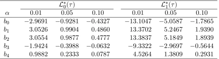
4.1 Response surface critical values
Clearly, L0( ) and L1( ) depend on . Hence, as in KY, we use a response surface to provide asymptotic null critical values. To accomplish this we simulated (upper tail) -level critical values for the limit distributions L0( )and L1( ). These were obtained by direct simulation of the limiting distributions above for the grid of values 2 f0:01;0:02; :::;0:99g, approximating the Brownian motion processes usingN IID(0;1)random variates, and with the integrals approximated by normalized sums of 2000 steps, and using 50,000 Monte Carlo replications. Denoting a simulated critical value ascv( )
we then ran the discretised OLS regression
cv( ) =b0+b1fh( ) + 1g 1+b2h( ) +b3h( )2+b4h( )3+error
with h( ) = j 0:5j, adopting the functional form used in KY. The parameter estimates are shown in Table 1 for L0( )and L1( )and = 0:01;0:05;0:10 and for each regression we …ndR2 >0:9995.
Hence, if the …tted critical values are applied to each of the sequence of tests !"2S0( ) under I(0)
[image:4.595.120.478.505.602.2]errors, and !u2fS1( ) 2ug under I(1) errors across , the corresponding con…dence set based on inverting these tests will have asymptotically correct coverage.
Table 1. Response surface parameter estimates
L0( ) L1( )
0.01 0.05 0.10 0.01 0.05 0.10
b0 2.9691 0.9281 0.4327 13.1047 5.0587 1.7865
b1 3.0526 0.9904 0.4860 13.3702 5.2467 1.9390
b2 3.0554 0.9877 0.4777 13.3837 5.1849 1.8939
b3 1.9424 0.3988 0.0632 9.3322 2.9697 0.5644
b4 0.9882 0.2333 0.0787 4.5264 1.3809 0.2931
5
Feasible tests and con…dence set selection
Feasible variants of S0( ) and S1( ) require an estimator of !2" for the former, and !2u and 2u for the latter. We employ the same estimators as favoured by HL in the context of S0( ) and S1( ).
These are the estimators!^2";P(^Dm),!^u;P2 (^Dm) and ^2u(^Dm) of that paper. The …rst two are Berk-type parametric autoregressive spectral density estimators. Each of the three estimators is based on residuals from a regression that incorporates a level/trend break …tted at same estimated break fraction ^Dm, where ^Dm is the estimator of 0 suggested by Harvey and Leybourne (2014). More
detail of the construction of this estimator can be found in HL, section 3.2. The feasible tests are then
^
In practice, the order of integration of the errors is unknown, and therefore a method is required to be able to choose between theI(0)-based con…dence set associated withS^ ^
0;P( )and theI(1)-based con…dence set for S^1;P^ ( ). In line with HL, section 4, we employ a pre-test for the null of = 1
against the alternative of j j < 1, which is robust to the possible presence of a break in level and trend. Practically, this involves running the left-tailed unit root single break MDF test of Harvey et al. (2013), then selecting the S^0;P^ ( ) con…dence set if MDF < cv and the S^1;P^ ( ) con…dence set if MDF cv , where cv denotes the asymptotic -level unit root null critical value of MDF. We denote this pre-test based procedure asS^pre;P^ ( ).
6
Finite sample comparisons
We now examine how con…dence sets which are based onS^pre;P^ ( )compare with those ofS^pre;P^ ( ), its counterpart from HL. In terms of their construction, it is important to remember the only di¤erence between the new tests and their forebears in HL lies in the modi…cation toHd;b Tc(and the consequent change to the ^2u(^Dm)centering in S^1;P^ ( )). As regards other settings relevant to both sets of tests, the number of lagged di¤erence terms in the …tted autoregressions that underpin !^2";P(^Dm) and
^
!2u;P(^Dm) is selected via the BIC with maximum value `max = 12(T =100)1=4 . The same value
`max is employed by the MAIC procedure of Perron and Qu (2007) to determine the length used by
the unit root test MDF. We adopt a 0.10 trimming for allowable break locations such that b Tc 2
fb0:1Tc; :::;b0:9Tcg; this same trimming is also imposed when constructing ^Dm andMDF. Each test (includingMDF) is conducted at the 0.05-level using the appropriate asymptotic critical value.
We simulate the DGP (1)-(2) with 1= 2= 0(without loss of generality) usingut N IID(0;1). The values of we consider for"tare 2 f0:00;0:50;0:80;0:90;0:95;1:00gto encompass a range ofI(0) processes and anI(1)process. As regards the break timings we use 02 f0:3;0:5;0:7g, corresponding
to early, middle and late sample breaks. The constellations we adopt for break magnitudes are
( 1; 2) 2 f(3c1;0:3c2);(4c1;0:4c2);(5c1;0:5c2);(6c1;0:6c2)g with c1 =c2 = 1 representing a break in
both level and trend (Table 2); c1 = 1; c2 = 0a break in level alone (Table 3); c1 = 0; c2 = 1a break
in trend alone (Table 4). Sample sizes are set at T = 150and T = 300.
All simulations are performed using 10,000 Monte Carlo replications, and we report results for con…dence set coverage (the proportion of replications for which the true break date is contained in the con…dence set) and con…dence set length (in each replication, length is calculated as the number of dates included in the con…dence set as a proportion of the sample size; we then report the average length over Monte Carlo replications). In what follows, we adopt a shorthand notation using S and
S to denoteS^pre;P^ ( )and S^pre;P^ ( ), respectively.
Consider …rst the coverage rates of S and S . Tables 2-4 show that there is very little to choose betweenSand S in terms of their levels of accuracy, and in general, both tests deliver coverage rates either close to the nominal level or higher. When = 1:00 and a break of small magnitude is present, both tests su¤er from some degree of under-coverage, particularly when only a trend break occurs. Here, S can exhibit slightly more under-coverage than S when 0 = 0:50;although for T = 300 the
di¤erences are small. The reverse pattern is true when = 0:00 and only a trend break occurs, with
S often being slightly under-sized whileS retains coverage close to 0.95. Overall, the picture is one of decent coverage across the di¤erent settings, with little di¤erence between S and S .
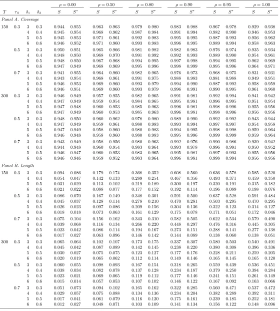
We now turn to comparing the con…dence set lengths. In Table 2, when T = 150and = 0:00 or
= 0:50, S generally yields the shorter lengths for 0 = 0:3and 0 = 0:5, while S yields the shorter
lengths for 0 = 0:7. The di¤erences are small, however, as both procedures give short con…dence
overall shortening of all the con…dence sets since the individual tests reject more frequently underH1.
Here, we now see that S provides systematically shorter con…dence sets than S for > 0:80. The improvements a¤orded byS are now commonly in the range of 0.05-0.10, which is obviously a lower range than for T = 150, but still not insubstantial.
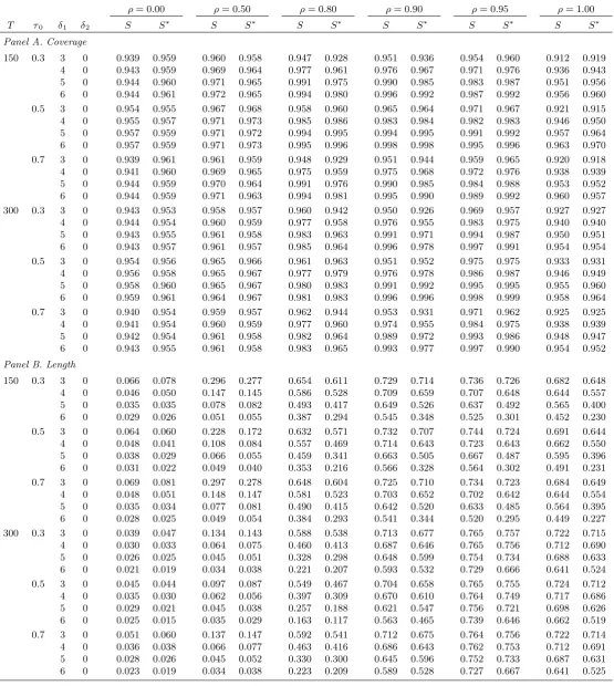
In Table 3 the lengths for bothS andS are generally larger than in Table 2, as would be expected since the trend break is now absent, lowering rejection frequencies underH1. What is also evident is
that when = 1:00, shorter lengths are obtained with T = 150 than withT = 300, due to the fact that a …xed magnitude level break is asymptotically undetectable in anI(1)process. We see a similar, but less emphasized, phenomenon with = 0:95, which might be considered a “near I(1)” process in the current context. Comparing S and S , the two are similar for = 0:00 or = 0:50, while S
always yields the shorter con…dence set for >0:50 forT = 150 and T = 300. Shortenings of up to about 0.25 are seen whenT = 150, with many in the range 0.15-0.20. WhenT = 300, the shortenings are less pronounced, but can still comfortably exceed 0.10 in some cases.
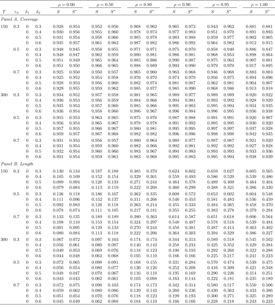
The same broad comparison betweenSandS also pertains to Table 4, withS generally providing the shorter lengths for >0:50. Interestingly, despite overall lengths here tending to exceed those in Table 2 due to the absence of the level break, the extent to which S reduces length appears rather less substantial, although gains in the range of 0.05-0.10 do still frequently occur.
In summary then, it is clear that the new procedureS can result in shorter con…dence sets than the original procedure S. While there is some ambiguity as to whether any gains fromS are meaningful for small values of , for the larger values of they can be considerable (particularly in a model which contains both a level and trend break). From an empirical perspective, that the better gains are made for moderately persistent I(0) processes to highly persistent I(1) processes is of some relevance, as these kinds of persistent series are often encountered in applied macroeconomic and …nancial time series analysis. At the slight expense of introducing location dependent asymptotic critical values (which are easily made accessible via a response surface), use ofS compared to Scan improve length with little impact on coverage rates, and we therefore recommend the modi…ed procedure for empirical work.
References
Elliott, G. and Müller, U.K. (2007). Con…dence sets for the date of a single break in linear time series regressions. Journal of Econometrics 141, 1196-1218.
Grenander, U. and Rosenblatt, M. (1957). Statistical Analysis of Stationary Time Series, John Wiley, New York.
Harvey, D.I. and Leybourne, S.J. (2014). Break date estimation for models with deterministic struc-tural change. Oxford Bulletin of Economics and Statistics 76, 623-642.
Harvey, D.I., Leybourne, S.J. and Taylor, A.M.R. (2013). Testing for unit roots in the possible pres-ence of multiple trend breaks using minimum Dickey-Fuller statistics. Journal of Econometrics, 177, 265-284.
Harvey, D.I. and Leybourne, S.J. (2015). Con…dence sets for the date of a break in level and trend when the order of integration is unknown. Journal of Econometrics 184, 262-279.
Kurozumi, E. and Yamamoto, Y. (2015). Con…dence sets for the break date based on optimal tests. Econometrics Journal 18, 412-435.
Table 2. Finite sample coverage and length of nominal 0.95-level confidence sets.
ρ= 0.00 ρ= 0.50 ρ= 0.80 ρ= 0.90 ρ= 0.95 ρ= 1.00
T τ0 δ1 δ2 S S∗ S S∗ S S∗ S S∗ S S∗ S S∗
Panel A. Coverage
150 0.3 3 0.3 0.944 0.955 0.963 0.963 0.979 0.980 0.983 0.988 0.967 0.978 0.929 0.938 4 0.4 0.945 0.954 0.968 0.962 0.987 0.984 0.991 0.994 0.982 0.990 0.946 0.953 5 0.5 0.945 0.953 0.971 0.961 0.992 0.983 0.995 0.995 0.987 0.993 0.956 0.962 6 0.6 0.946 0.952 0.971 0.960 0.993 0.983 0.996 0.995 0.989 0.994 0.958 0.963 0.5 3 0.3 0.950 0.951 0.965 0.966 0.981 0.982 0.982 0.983 0.976 0.974 0.935 0.934 4 0.4 0.948 0.950 0.968 0.970 0.991 0.992 0.992 0.993 0.989 0.990 0.954 0.961 5 0.5 0.948 0.950 0.967 0.968 0.994 0.995 0.997 0.998 0.994 0.995 0.962 0.969 6 0.6 0.947 0.949 0.968 0.969 0.995 0.996 0.998 0.999 0.995 0.996 0.964 0.971 0.7 3 0.3 0.941 0.955 0.964 0.960 0.982 0.965 0.976 0.973 0.968 0.975 0.931 0.931 4 0.4 0.943 0.954 0.968 0.961 0.991 0.975 0.988 0.983 0.981 0.988 0.949 0.951 5 0.5 0.946 0.953 0.969 0.960 0.993 0.979 0.994 0.990 0.987 0.992 0.958 0.959 6 0.6 0.946 0.951 0.969 0.960 0.993 0.979 0.996 0.991 0.990 0.995 0.961 0.960 300 0.3 3 0.3 0.946 0.949 0.957 0.955 0.982 0.965 0.991 0.981 0.992 0.994 0.941 0.942 4 0.4 0.947 0.949 0.959 0.954 0.984 0.965 0.995 0.981 0.996 0.995 0.951 0.954 5 0.5 0.947 0.948 0.960 0.953 0.985 0.963 0.996 0.981 0.998 0.996 0.955 0.956 6 0.6 0.947 0.949 0.960 0.953 0.985 0.963 0.996 0.981 0.998 0.996 0.956 0.956 0.5 3 0.3 0.948 0.950 0.960 0.962 0.978 0.980 0.989 0.990 0.992 0.992 0.943 0.944 4 0.4 0.947 0.949 0.959 0.961 0.980 0.983 0.993 0.994 0.997 0.997 0.954 0.958 5 0.5 0.947 0.949 0.958 0.960 0.980 0.983 0.994 0.995 0.998 0.998 0.959 0.964 6 0.6 0.946 0.948 0.958 0.960 0.980 0.983 0.995 0.996 0.999 0.999 0.959 0.964 0.7 3 0.3 0.943 0.949 0.958 0.956 0.980 0.963 0.992 0.976 0.990 0.986 0.939 0.942 4 0.4 0.944 0.948 0.960 0.954 0.983 0.964 0.993 0.978 0.996 0.991 0.950 0.952 5 0.5 0.946 0.947 0.960 0.953 0.983 0.965 0.995 0.981 0.997 0.993 0.955 0.956 6 0.6 0.946 0.946 0.959 0.952 0.983 0.964 0.996 0.981 0.998 0.994 0.956 0.956
Panel B. Length
Table 3. Finite sample coverage and length of nominal 0.95-level confidence sets.
ρ= 0.00 ρ= 0.50 ρ= 0.80 ρ= 0.90 ρ= 0.95 ρ= 1.00
T τ0 δ1 δ2 S S∗ S S∗ S S∗ S S∗ S S∗ S S∗
Panel A. Coverage
150 0.3 3 0 0.939 0.959 0.960 0.958 0.947 0.928 0.951 0.936 0.954 0.960 0.912 0.919 4 0 0.943 0.959 0.969 0.964 0.977 0.961 0.976 0.967 0.971 0.976 0.936 0.943 5 0 0.944 0.960 0.971 0.965 0.991 0.975 0.990 0.985 0.983 0.987 0.951 0.956 6 0 0.944 0.961 0.972 0.965 0.994 0.980 0.996 0.992 0.987 0.992 0.956 0.960 0.5 3 0 0.954 0.955 0.967 0.968 0.958 0.960 0.965 0.964 0.971 0.967 0.921 0.915 4 0 0.955 0.957 0.971 0.973 0.985 0.986 0.983 0.984 0.982 0.983 0.946 0.950 5 0 0.957 0.959 0.971 0.972 0.994 0.995 0.994 0.995 0.991 0.992 0.957 0.964 6 0 0.957 0.959 0.971 0.973 0.995 0.996 0.998 0.998 0.995 0.996 0.963 0.970 0.7 3 0 0.939 0.961 0.961 0.959 0.948 0.929 0.951 0.944 0.959 0.965 0.920 0.918 4 0 0.941 0.960 0.969 0.965 0.975 0.959 0.975 0.968 0.972 0.976 0.938 0.939 5 0 0.944 0.959 0.970 0.964 0.991 0.976 0.990 0.985 0.984 0.988 0.953 0.952 6 0 0.944 0.959 0.971 0.963 0.994 0.981 0.995 0.990 0.989 0.992 0.960 0.957 300 0.3 3 0 0.943 0.953 0.958 0.957 0.960 0.942 0.950 0.926 0.969 0.957 0.927 0.927 4 0 0.944 0.954 0.960 0.959 0.977 0.958 0.976 0.955 0.983 0.975 0.940 0.940 5 0 0.943 0.955 0.961 0.958 0.983 0.963 0.991 0.971 0.994 0.987 0.950 0.951 6 0 0.943 0.957 0.961 0.957 0.985 0.964 0.996 0.978 0.997 0.991 0.954 0.954 0.5 3 0 0.954 0.956 0.965 0.966 0.961 0.963 0.951 0.952 0.975 0.975 0.933 0.931 4 0 0.956 0.958 0.965 0.967 0.977 0.979 0.976 0.978 0.986 0.987 0.946 0.949 5 0 0.958 0.960 0.965 0.967 0.980 0.983 0.991 0.992 0.995 0.995 0.955 0.960 6 0 0.959 0.961 0.964 0.967 0.981 0.983 0.996 0.996 0.998 0.999 0.958 0.964 0.7 3 0 0.940 0.954 0.959 0.957 0.962 0.944 0.953 0.931 0.971 0.962 0.925 0.925 4 0 0.941 0.954 0.960 0.959 0.977 0.960 0.974 0.955 0.984 0.975 0.938 0.939 5 0 0.942 0.954 0.961 0.958 0.982 0.964 0.989 0.972 0.993 0.986 0.948 0.947 6 0 0.943 0.955 0.961 0.958 0.983 0.965 0.993 0.977 0.997 0.990 0.954 0.952
Panel B. Length
Table 4. Finite sample coverage and length of nominal 0.95-level confidence sets.
ρ= 0.00 ρ= 0.50 ρ= 0.80 ρ= 0.90 ρ= 0.95 ρ= 1.00
T τ0 δ1 δ2 S S∗ S S∗ S S∗ S S∗ S S∗ S S∗
Panel A. Coverage
150 0.3 0 0.3 0.928 0.954 0.952 0.956 0.968 0.962 0.965 0.973 0.943 0.962 0.881 0.881 0 0.4 0.930 0.956 0.955 0.960 0.978 0.974 0.977 0.983 0.951 0.970 0.891 0.893 0 0.5 0.931 0.954 0.958 0.960 0.985 0.978 0.983 0.988 0.959 0.977 0.902 0.905 0 0.6 0.935 0.957 0.961 0.962 0.987 0.982 0.986 0.992 0.964 0.982 0.912 0.915 0.5 0 0.3 0.948 0.945 0.958 0.955 0.971 0.971 0.975 0.970 0.958 0.940 0.886 0.847 0 0.4 0.948 0.947 0.962 0.959 0.980 0.981 0.986 0.981 0.968 0.953 0.898 0.864 0 0.5 0.951 0.949 0.965 0.964 0.985 0.986 0.990 0.987 0.975 0.963 0.907 0.881 0 0.6 0.951 0.950 0.966 0.965 0.988 0.989 0.993 0.990 0.979 0.970 0.917 0.895 0.7 0 0.3 0.925 0.950 0.950 0.957 0.965 0.960 0.963 0.968 0.946 0.968 0.883 0.883 0 0.4 0.925 0.952 0.954 0.958 0.976 0.970 0.974 0.979 0.956 0.975 0.894 0.896 0 0.5 0.928 0.953 0.956 0.960 0.982 0.974 0.981 0.987 0.962 0.981 0.904 0.907 0 0.6 0.929 0.955 0.959 0.962 0.985 0.977 0.985 0.990 0.968 0.986 0.913 0.918 300 0.3 0 0.3 0.934 0.952 0.957 0.958 0.981 0.965 0.989 0.977 0.989 0.989 0.920 0.922 0 0.4 0.936 0.953 0.956 0.959 0.984 0.966 0.994 0.981 0.993 0.992 0.928 0.929 0 0.5 0.935 0.953 0.957 0.960 0.985 0.966 0.995 0.983 0.995 0.994 0.934 0.935 0 0.6 0.936 0.954 0.958 0.960 0.986 0.967 0.996 0.984 0.996 0.995 0.936 0.938 0.5 0 0.3 0.955 0.953 0.963 0.965 0.975 0.976 0.987 0.988 0.991 0.991 0.920 0.907 0 0.4 0.956 0.954 0.965 0.967 0.978 0.978 0.991 0.992 0.995 0.995 0.930 0.920 0 0.5 0.957 0.955 0.966 0.967 0.980 0.981 0.995 0.995 0.997 0.997 0.937 0.928 0 0.6 0.959 0.957 0.967 0.968 0.982 0.982 0.996 0.996 0.998 0.998 0.942 0.935 0.7 0 0.3 0.931 0.953 0.956 0.957 0.980 0.964 0.989 0.977 0.987 0.987 0.921 0.920 0 0.4 0.931 0.954 0.959 0.960 0.982 0.966 0.992 0.981 0.992 0.992 0.927 0.928 0 0.5 0.932 0.954 0.960 0.960 0.983 0.967 0.994 0.983 0.993 0.993 0.933 0.936 0 0.6 0.931 0.954 0.959 0.961 0.983 0.968 0.995 0.983 0.995 0.994 0.938 0.939
Panel B. Length