Macroscopic coherent structures in a stochastic neural network: from interface dynamics to coarse grained bifurcation analysis

MACROSCOPIC COHERENT STRUCTURES IN A STOCHASTIC NEURAL NETWORK: FROM INTERFACE DYNAMICS TO

COARSE-GRAINED BIFURCATION ANALYSIS.

DANIELE AVITABILE ∗ AND KYLE WEDGWOOD †

Abstract. We study coarse pattern formation in a cellular automaton modelling a spatially-extended stochastic neural network. The model, originally proposed by Gong and Robinson [36], is known to support stationary and travelling bumps of localised activity. We pose the model on a ring and study the existence and stability of these patterns in various limits using a combination of analytical and numerical techniques. In a purely deterministic version of the model, posed on a continuum, we construct bumps and travelling waves analytically using standard interface methods from neural fields theory. In a stochastic version with Heaviside firing rate, we construct approxi-mate analytical probability mass functions associated with bumps and travelling waves. In the full stochastic model posed on a discrete lattice, where a coarse analytic description is unavailable, we compute patterns and their linear stability using equation-free methods. The lifting procedure used in the coarse time-stepper is informed by the analysis in the deterministic and stochastic limits. In all settings, we identify the synaptic profile as a mesoscopic variable, and the width of the correspond-ing activity set as a macroscopic variable. Stationary and travellcorrespond-ing bumps have similar meso- and macroscopic profiles, but different microscopic structure, hence we propose lifting operators which use microscopic motifs to disambiguate between them. We provide numerical evidence that waves are supported by a combination of high synaptic gain and long refractory times, while meandering bumps are elicited by short refractory times.

1. Introduction. In the past decades, single-neuron recordings have been com-plemented by multineuronal experimental techniques, which have provided quanti-tative evidence that the cells forming the nervous systems are coupled both struc-turally [8] and functionally (for a recent review, see [75] and references therein). An important question in neuroscience concerns the relationship between electrical ac-tivity at the level of individual neurons and the emerging spatio-temporal coherent structures observed experimentally using local field potential recordings [22], func-tional magnetic resonance imaging [69] and electroencephalography [58].

There exist a wide variety of models describing activity at the level of an indi-vidual neuron [39, 26], and major research efforts in theoretical and computational neuroscience are directed towards coupling neurons in large-dimensional neural net-works, whose behaviour is studied mainly via direct numerical simulations [40,27].

A complementary approach, dating back to Wilson and Cowan [73, 74] and Amari [1, 2], foregoes describing activity at the single neuron level by represent-ing averaged activity across populations of neurons. These neural field models are nonlocal, spatially-extended, excitable pattern-forming systems [24] which are of-ten analytically tractable and support several coherent structures such as localised radially-symmetric states [72, 54, 52, 14, 29], localised patches [53, 63, 4], patterns on lattices with various symmetries [23, 13], travelling bumps and fronts [25, 12], rings [61,19], breathers [30,31,32], target patterns [20], spiral waves [47] and lurch-ing waves [35, 60,71] (for comprehensive reviews, we refer the reader to [11,12]).

Recent studies have analysed neural fields with additive noise [38,28,46], multi-plicative noise [15], or noisy firing thresholds [7], albeit these models are still mostly phenomenological. Even though several papers derive continuum neural fields from

∗_{Centre for Mathematical Medicine and Biology, School of Mathematical Sciences, University of} Nottingham, Nottingham, NG2 7RD, UK

microscopic models of coupled neurons [41, 9, 10, 5], the development of a rigorous theory of multi-scale brain models is an active area of research.

Numerical studies of networks based on realistic neural biophysical models rely almost entirely on brute-force Monte Carlo simulations (for a very recent, remarkable example, we refer the reader to [56]). With thisdirect numerical simulation approach, the stochastic evolution of each neuron in the network is monitored, resulting in huge computational costs, both in terms of computing time and memory. From this point of view, multi-scale numerical techniques for neural networks present interesting open problems.

When few clusters of neurons with similar properties form in the network, a significant reduction in computational costs can be obtained by population density methods [59,37], which evolve probability density functions of neural subpopulations, as opposed to single neuron trajectories. This coarse-graining technique is particularly effective when the underlying microscopic neuronal model has a low-dimensional state space (such as the leaky integrate-and-fire model) but its performance degrades for more realistic biophysical models. Developments of the population density method involve analytically derived moment closure approximations [16, 55]. Both Monte Carlo simulations and population density methods give access only to stable asymp-totic states, which may form only after long-transient simulations.

An alternative approach is offered by equation-free [42, 43] and heterogeneous multiscale methods [70,21], which implement multiple-scale simulations using an on-the-fly numerical closure approximations. Equation-free methods, in particular, are of interest in computational neuroscience as they accelerate macroscopic simulations and allow the computation of unstable macroscopic states. In addition, with equation-free methods, it is possible to perform coarse-grained bifurcation analysis using standard numerical bifurcation techniques for time-steppers [68].

The equation-free framework [42, 43] assumes the existence of a closed coarse model in terms of a few macroscopic state variables. The model closure is enforced numerically, rather than analytically, using a coarse time-stepper: a computational procedure which takes advantage of knowledge of the microscopic dynamics to time-step an approximated macroscopic evolution equation. A single coarse time time-step from time t0 to time t1 is composed of three stages: (i) lifting, that is, the creation of

microscopic initial conditions that are compatible with the macroscopic states at time t0; (ii)evolution, the use of independent realisations of the microscopic model over a

time interval [t0, t1]; (iii)restriction, that is, the estimation of the macroscopic state

at timet1using the realisations of the microscopic model.

While equation-free methods have been employed in various contexts (see [43] and references therein) and in particular in neuroscience applications [48,50,49,66,

67,51], there are still open questions, mainly related to how noise propagates through the coarse time stepper. A key aspect of every equation-free implementation is the lifting step. The underlying lifting operator, which maps a macroscopic state to a set of microscopic states, is generally non-unique, and lifting choices have a considerable impact on the convergence properties of the resulting numerical scheme [3]. Even though the choice of coarse variables can be automatised using data-mining tech-niques, as shown in several papers by Laing, Kevrekidis and co-workers [48, 50,49], the lifting step is inherently problem dependent.

The present paper explores the possibility of using techniques from neural field models to inform the coarse-grained bifurcation analysis of discrete neural networks. A successful strategy in analysing neural fields is to replace the models’ sigmoidal

firing rate functions with Heaviside distributions [11, 12]. Using this strategy, it is possible to relate macroscopic observables, such as bump widths or wave speeds, to biophysical parameters, such as firing rate thresholds. Under this hypothesis, a macroscopic variable suggests itself, as the state of the system can be constructed entirely via the loci of points in physical space where the neural activity attains the firing-rate threshold value. In addition, there exists a closed (albeit implicit) evolution equation for such interfaces [19].

In this study, we show how the insight gained in the Heaviside limit may be used to perform coarse-grained bifurcation analysis of neural networks, even in cases where the network does not evolve according to an integro-differential equation. As an illustrative example, we consider a spatially-extended neural network in the form of a discrete time Markov chain with discrete ternary state space, posed on a lattice. The model is an existing cellular automaton proposed by Gong and co-workers [36], and it has been related to neuroscience in the context of relevant spatio-temporal activity patterns that are observed in cortical tissue. In spite of its simplicity, the model possesses sufficient complexity to support rich dynamical behaviour akin to that produced by neural fields. In particular, it explicitly includes refractoriness and is one of the simplest models capable of generating propagating activity in the form of travelling waves. An important feature of this model is that the microscopic transition probabilities depend on the local properties of the tissue, as well as on the global synaptic profile across the network. The latter has a convolution structure typical of neural field models, which we exploit to use interface dynamics and define a suitable lifting strategy.

To connect our micro- and macroscopic variables, we take advantage of interface approaches, which are typically applied to continuum networks. A notable exception is offered by Chow and Coombes [?], who consider a network based upon the light-house model [?]. In a similar vein to our approach, they show how analysis of the discrete network can be facilitated by considering a continuum approximation and de-rive threshold equations to define bump solutions. This analysis also highlights that perturbations to the microscopic state, specifically the phase arrangement within the bump, can alter the dynamics of the bump edges.

Chow and Coombes found that wandering bump solutions in the lighthouse model arise for sufficiently fast synaptic processing. This is congruent with our result that short refractory times in (2.8) elicit coherent bump states, since both refractory times and synaptic processing timescales affect the average firing rate of the neuron. How-ever, bumps cease to exist in our model if the refractory times are too long, whereas the lighthouse model supports stationary bumps for slow synapses, which highlights the subtle differences between the roles of refractoriness and synaptic processing in neural networks. It should also be noted that the meandering observed, for instance, in Figure 2 is due to noise, and that all bumps will tend to wander; on the other hand, the meandering described by Chow and Coombes arises from the deterministic dynamics of the lighthouse model, and it is triggered by a sufficently fast synaptic process. We also remark that, without modification, the lighthouse model does not support travelling wave solutions, and so we cannot make comparisons regarding these solutions.

cor-responding lifting operators, which highlight a critical importance of the microscopic structure of solutions: one of the main results of our analysis is that, since macroscopic stationary and travelling bumps coexist and have nearly identical macroscopic profiles, a standard lifting is unable to distinguish between them, thereby preventing coarse numerical continuation. These structures, however, possess different microstructures, which are captured by our analysis and subsequently by our lifting operators. This allows us to compute separate solution branches, in which we vary several model parameters, including those associated with the noise processes.

The manuscript is arranged as follows: In Section 2 we outline the model. In Section 3, we simulate the model and identify the macroscopic profiles in which we are interested, together with the coarse variables that describe them. In Section 4, we define a deterministic version of the full model and lay down the framework for analysing it. In Sections5and6, we respectively construct bump and wave solutions under the deterministic approximation and compute the stability of these solutions. In Section7, we define and construct travelling waves relaxing the deterministic limit. In Sections8.1and8.2, we provide the lifting steps for use in the equation-free algorithm for the bump and wave respectively. In Section9, we briefly outline the continuation algorithm and in Section10, we show the results of applying this continuation to our system. Finally, in Section11, we make some concluding remarks.

2. Model description.

2.1. State variables for continuum and discrete tissues. In this section, we present a modification of a model originally proposed by Gong and Robinson [36]. We consider a one-dimensional neural tissueX⊂R. At each discrete time stept∈Z, a neuron at positionx_∈Xmay be in one of three states: a refractory state (henceforth denoted as₋1), a quiescent state (0) or a spiking state (1). Our state variable is thus a functionu:X×Z→U, whereU={ −1,0,1}. We pose the model on a continuum tissueS=R/2LZor on a discrete tissue featuringN+ 1 evenly spaced neurons,

SN ={xi}Ni=0, xi=−L+i2L/N ∈[−L, L].

We will often alternate between the discrete and the continuum setting, hence we will use a unified notation for these cases. We use the symbolXto refer to eitherSorSN, depending on the context. Also, we use u(_·, t) to indicate the state variable in both the discrete and the continuum case: u(_·, t) will denote a step function defined onS in the continuum case and a vector in UN with components u(xi, t) in the discrete case. Similarly, we writeR

Xu(x) dxto indicate

R

Su(x) dxor 2L/N

PN

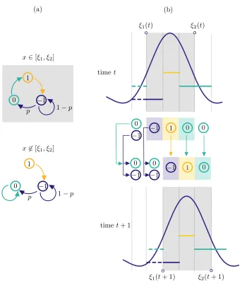
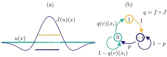
j=0u(xj). 2.2. Model definition. We use the term stochastic model when the Markov chain model described below is posed onSN. An example of a state supported by the stochastic model is given in Figure1(a).

In the model, neurons are coupled via a translation-invariant synaptic kernel, that is, we assume the connection strength between two neurons to be dependent on their mutual Euclidean distance. In particular, we prescribe that short range connections are excitatory, whilst long-range connections are inhibitory. To model this coupling, we use a standard Mexican hat function,

(2.1) w:X→R, x7→A1

p

B1/Lexp(−4B1x2)−A2

p

B2/Lexp(−4B2x2),

and denote byW its periodic extension.

(a) (b)

1

1 0

1 p

1

p u(x)

q(v)(xi)

1 q(v)(xi) J(u)(x)

q=f J

Fig. 1.(a): Example of a stateu(x)∈UN and corresponding synaptic profileJ(u)(x)∈RNin

a stochastic network of1024neurons. (b): Schematic of the transition kernel for the network (see also Equations (2.5)–(2.7)). The conditional probability of the local variableu(xi, t+ 1)depends on

the global state of the network at timet, via the functionq=f◦J, as seen in (2.7).

In order to describe the dynamics of the model, it is useful to partition the tissue Xinto the 3 pullback sets

(2.2) Xku(t) ={x∈X:u(x, t) =k}, k∈U, t∈Z,

so that we can write, for instance,Xu

1(t) to denote the set of neurons that are firing

at timet(and similarly forXu

−1andX0u). Where it is unambiguous, we shall simply

writeXk orXk(t) in place of Xu k(t).

The synaptic input to a cell at position xi is given by a weighted sum of inputs from all firing cells. Using the synaptic kernel (2.1) and the partition (2.2), the synaptic input is then modelled as

(2.3) J:X×Z→R, (x, t)7→κ Z

X

W(x−y)1X1(t)(y) dy=κ

Z

X1(t)

W(x−y)dy,

where κ_∈R+ is the synaptic gain, which is common for all neurons and 1X is the indicator function of a setX.

Remark 2.1 (Synaptic input as mesoscopic variable). Since X1 depends on the microscopic state variable u, so does the synaptic input (2.3). Where necessary, we will writeJ(u)(x, t)to highlight the dependence onu. We refer the reader to Figure1

for a concrete example of synaptic profile.

The firing probability associated to a quiescent neuron is linked to the synaptic input via the firing rate function

(2.4) f: R→R, I7→ 1

1 + exp[−β(I−h)],

probabilities specified as follows: for eachxi_∈SN andt∈Z

Pr

u(xi, t+ 1) =₋1

u(x, t) =v(x)

=   

 

1−p ifv(xi) =−1, 1 ifv(xi) = 1, 0 otherwise, (2.5)

Pr

u(xi, t+ 1) = 0

u(x, t) =v(x)

=   

 

p ifv(xi) =₋1,

1−f(J(v))(xi) ifv(xi) = 0,

0 otherwise,

(2.6)

Pr

u(xi, t+ 1) = 1

u(x, t) =v(x)

= (

f(J(v))(xi) ifv(xi) = 0,

0 otherwise,

(2.7)

wherep∈(0,1]. We give a schematic representation of the transitions of each neuron in the network in Figure 1(b). We remark that conditional probability of the local

variable u(xi, t+ 1) depends on the global state of the network at time t, via the functionf◦J.

The model described by (2.1)–(2.7), complemented by initial conditions, defines a stochastic evolution map that we will formally denote as

(2.8) u(x, t+ 1) =ϕ(u(x, t);γ),

whereγ= (κ, β, h, p, A1, A2, B1, B2) is a vector of control parameters.

Remark 2.2 (Microscopic, mesoscopic and macroscopic descriptions). We will henceforth use the terms “microscopic”, “mesoscopic” and “macroscopic” to refer to different state variables or model descriptions. Examples of these three state variables appear toghether in Figures2–4in Section3, and we introduce them briefly here: Microscopic level. Model (2.8)will be referred to as microscopic model and its

so-lutions at a fixed time t as microscopic states. We will use these terms also whenp= 1andβ → ∞, that is, when the evolution equation (2.8)is deter-ministic.

Mesoscopic level. In Remark2.1, we associated to each microscopic stateua corre-sponding synaptic profileJ, which is smooth, even when the tissue is discrete. We will not seek for an evolution equation for the variable J, as the corre-sponding dynamical system would not reprent a reduction of the microscopic one. However, we will use J to bridge between the microscopic and macro-scopic model descriptions; we therefore refer to J as a mesoscopic variable (or mesoscopic state).

Macroscopic level. Much of the present paper aims to show that, for the model un-der consiun-deration, there exists a high-level model description, in the spirit of interfacial dynamics for neural fields [11,19,12]. The state variables for this level are points on the tissue whereJ(u)(x, t)attains the firing rate threshold

h. We will denote these threshold crossings as_{ξi(t)}and we will discuss (re-duced) evolution equations in terms ofξi(t). The variables_{ξ(t)}are therefore referred to as macroscopic variables and the corresponding evolution equations as macroscopic model.

3. Microscopic states observed via direct simulation. In this section, we introduce a few coherent states supported by the stochastic model. The main aim of the section is to show examples of bumps, multiple bumps and travelling waves, whose existence and stability properties will be studied in the following sections. In

Experiment κ β h p A1 A2 B1 B2 N L

Bump 30 5 0.9 0.7 5.25 5 0.2 0.3 1024 π

Multiple bump 60 5 0.9 0.7 5.25 5 0.2 0.3 2058 2π

Travelling wave 30 ∞ 1.0 0.4 5.25 5 0.2 0.3 1024 π Table 1

Parameter values for which the stochastic model supports a bump (Figure2), a multiple-bump solution (Figure3) and a travelling wave (Figure4). The value∞for the parameter β indicates that a Heaviside firing rate has been used in place of the sigmoidal function (2.4).

addition, we give a first characterisation of the macroscopic variables of interest and link them to the microscopic structure observed numerically.

3.1. Bumps. In a suitable region of parameter space, the microscopic model supports bump solutions [62] in which the microscopic variableu(x, t) is nonzero only in a localised region of the tissue. In thisactive region, neurons attain all values in U. In Figure2, we show a time simulation of the microscopic model with N = 1024 neurons. At each time t, neurons are in the refractory (blue), quiescent (green) or spiking (yellow) state. We prescribe the initial condition by setting u(xi,0) = 0 outside of a localised region, in which u(xi,0) are sampled randomly from U. After a short transient, a stochastic microscopic bump is formed. As expected due to the stochastic nature of the system [45], the active region wanders while remaining localised. A space-time section of the active region reveals a characteristic random microstructure (see Figure 2(a)). By plotting J(x, t), we see that the active region is well approximated by the portion of the tissue X≥ = [ξ1, ξ2] where J lies above

the thresholdh. A quantitative comparison betweenJ(x,50) andu(x,50) is made in Figure2(a). We interpretJ as amesoscopic variable associated with the bump, and ξ1andξ2 as correspondingmacroscopic variables (see also Remark2.2).

3.2. Multiple-bumps solutions. Solutions with multiple bumps are also ob-served by direct simulation, as shown in Figure3. The microstructure of these patterns resembles the one found in the single bump case (see Figure3(a)). At the mesoscopic level, the set for whichJ lies above the thresholdhis now a union of disjoint intervals [ξ1, ξ2], . . . ,[ξ7, ξ8]. The number of bumps of the pattern depends on the width of the

tissue; the experiment of Figure 3 is carried out on a domain twice as large as that of Figure 2. The examples of bump and multiple-bump solutions reported in these figures are obtained for different values of the main control parameterκ(see Table1), however, these states coexist in a suitable region of parameter space, as will be shown below.

3.3. Travelling waves. Further simulation shows that the model also supports coherent states in the form of stochastic travelling waves. In two spatial dimensions, the system is known to support travelling spots [36,62]. In Figure4, we show a time simulation of the stochastic model with initial condition

u(x,0) =X k∈U

k1Xk(x) with partition

X−1= [−1.5,−0.5),

X0= [−π,−1.5)∪[0.5, π),

X1= [−0.5,0.5).

(a)

x

−π π

u(x,50) J(x,50) 5

0

0 t

0 t

100 100

0

−1 3.5 (b)

x

−π π −π x π

ξ1 ξ2

J

1 0 1 u

Fig. 2.Bump obtained via time simulation of the stochastic model for(x, t)∈[−π, π]×[0,100].

(a): The microscopic state u(x, t) (left) attains the discrete values −1 (blue), 0 (green) and 1

(yellow). The corresponding synaptic profileJ(x, t)is a continuous function. A comparison between

J(x,50)and u(x,50)is reported on the right panel, where we also mark the interval[ξ1, ξ2]where J is above the firing thresholdh. (b): Space-time plots ofuandJ. Parameters as in Table1.

In the direct simulation of Figure 4, the active region moves to the right and, after just 4 iterations, a travelling wave emerges. The microscopic variable, u(x, t), displays stochastic fluctuations which disappear at the level of the mesoscopic variable, J(x, t), giving rise to a seemingly deterministic travelling wave. A closer inspection (Figure4(a)) reveals that the state can still be described in terms of the active region [ξ1, ξ2] whereJ is aboveh. However, the travelling wave has a different microstructure

with respect to the bump. Proceeding from right to left, we observe:

1. A region of the tissue ahead of the wave, x∈(ξ2, π), where the neurons are

in the quiescent state 0 with high probability.

2. An active regionx∈[ξ1, ξ2], split in three subintervals, each of approximate

width (ξ2−ξ1)/3, whereuattains with high probability the values 0, 1 and −1 respectively.

3. A region at the back of the wave, x ∈ [−π, ξ1), where neurons are either

quiescent or refractory. We note thatu= 0 with high probability asx_{→ −}π whereas, as x _→ ξ1, neurons are increasingly likely to be refractory, with

u=₋1.

(a)

0 t

0 t

100 100

(b)

x

0

−2 5 J

−2π 2π₋2π x 2π

2 0 2

−2π ξ1 ξ2 . . . ξ7 ξ82π

1 0 1 u

Fig. 3.Multiple bump solution obtained via time simulation of the stochastic model for(x, t)∈ [−2π,2π]×[0,100]. (a): The microscopic stateu(x, t)in the active region (left) is similar to the one found for the single bump (see Figure2(a)). A comparison betweenJ(x,50)andu(x,50)is reported on the right panel, where we also mark the intervals[ξ1, ξ2], . . . ,[ξ7, ξ8]whereJ is above the firing

thresholdh. (b): Space-time plots ofuandJ. Parameters are as in Table1.

A further observation of the space-time plot ofuin Figure4(b) reveals a remark-ably simple advection mechanism of the travelling wave, which can be fully understood in terms of the transition kernel of Figure 1(b) upon noticing that, for sufficiently largeβ, qi =f(J(u))(xi)_≈0 everywhere except in the active region, whereqi _≈1. In Figure5, we show how the transition kernel simplifies inside and outside the active region and provide a schematic of the advection mechanism. For an idealised trav-elling wave profile at time t, we depict 3 subintervals partitioning the active region (shaded), together with 2 adjacent intervals outside the active region. Each interval is then mapped to another interval, following the simplified transition rules sketched in Figure5(a):

1. At the front of the wave, to the right ofξ2(t), neurons in the quiescent state

0 remain at 0 (rules forx6∈[ξ1, ξ2]).

2. Inside the active region, to the left ofξ2(t), we follow the rules forx∈[ξ1, ξ2]

0 5

0

−2 5 (a)

(b)

50

0 t 50

0 t

−π π

J J(x,45)

u(x,45)

x

−π π−π x π

ξ1 x ξ2

1 0 1 u

Fig. 4.Travelling wave obtained via time simulation of the stochastic model for(x, t)∈[−π, π]× [0,50]. (a): The microscopic stateu(x, t)(left) has a characteristic microstructure, which is also visible on the right panel, where we compareJ(x,45)andu(x,45). As in the other cases, we mark the interval [ξ1, ξ2]where J is above the firing threshold h. (b): Space-time plots of u and J.

Parameters are as in Table1.

the neurons in the refractory state, those being the ones nearest ξ1(t), a

proportionpbecome quiescent, while the remaining ones remain refractory. 3. At the back of the wave, to the left ofξ1(t), the interval contains a mixture

of neurons in states 0 and−1. The former remain at 0 whilst, of the latter, a proportionptransition into state 0, with the rest remaining at−1 (rules for x6∈ [ξ1, ξ2]). From this argument, we see that the proportion of refractory

neurons in the back of the wave must decrease asξ→ −π.

The resulting mesoscopic variableJ(x, t+1) is a spatial translation by (ξ2(t)−ξ1(t))/3

ofJ(x, t). We remark that the approximate transition rules of Figure5(a) are valid also in the case of a bump, albeit the corresponding microstructure does not allow the advection mechanism described above.

3.4. Macroscopic variables. The computations of the previous sections sug-gest that, beyond the mesoscopic variable, J(x), coarser macroscopic variables are available to describe the observed patterns. In analogy with what is typically found in neural fields with Heaviside firing rate [2,12,18], the scalars_{ξi_}defining the active

(a) (b)

1

1 0

1 p

p

1

1 0

1 p

p x₂[⇠1, ⇠2]

x₆₂[⇠1, ⇠2]

timet

⇠1(t) ⇠2(t)

timet+ 1

⇠2(t+ 1)

⇠1(t+ 1)

0 1 1 0

1

0

1 0

1 0

1

0

1

Fig. 5. Schematic of the advection mechanism for the travelling wave state. Shaded areas

pertain to the active region [ξ1(t), ξ2(t)], non-shaded areas to the inactive region X\[ξ1(t), ξ2(t)].

(a): In the active (inactive) region,qi=f(J(u))(xi)≈1(qi≈0), hence the transition kernel(2.5)– (2.7)can be simplified as shown. (b): At timetthe travelling wave has a profile similar to the one in Figure4, which we represent in the proximity of the active region. We depict 5 intervals of equal width,3of which form a partition of[ξ1(t), ξ2(t)]. Each interval is mapped to another interval at

timet+ 1, following the transition rules sketched in (a). In one discrete step, the wave progresses with positive speed: so thatJ(x, t+ 1)is a translation ofJ(x, t).

regionX≥=∪i[ξ2i−1, ξ2i], whereJ is above h, seem plausible macroscopic variables.

This is evidenced not only by Figures2–4, but also from the schematic in Figure5(b), where the interval [ξ1(t), ξ2(t)] is mapped to a new interval [ξ1(t+ 1), ξ2(t+ 1)] of the

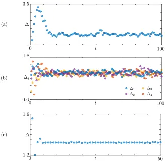
same width. To explore this further, we extract the widths ∆i(t) of each sub-interval [ξ2i(t), ξ2i−1(t)] from the data in Figure 2–4, and plot the widths as a function oft.

(a)

(b)

(c)

0 t 100

1 3.5

0.6 1.8

0 t 100

2

1 3

4

0 t

1.2 1.6 i

50

Fig. 6. Width of the active regions ∆i =ξ2i−ξ2i−1 for the patterns in Figures 2–4. (a):

Bump, for whichi= 1. (b): Multiple Bump,i= 1, . . . ,4. (c): Travelling wave,i= 1. In all cases, the patterns reach a coarse equilibrium state after a short transient.

intervals have approximately the same asymptotic width.

4. Deterministic model. We now introduce a deterministic version of the stochastic model considered in Section 2.2, which is suitable for carrying out ana-lytical calculations. We make the following assumptions:

1. Continuum neural tissue. We consider the limit of infinitely many neurons and pose the model onS.

2. Deterministic transitions. We assume p = 1, which implies a deterministic transition from refractory states to quiescent ones (see Equation (2.5)), and β _{→ ∞}, which induces a Heaviside firing rate f(I) = Θ(I₋h) and hence a deterministic transition from quiescent states to spiking ones given sufficiently high input (see Equations (2.4), (2.6)).

In addition to the pullback setsX−1,X0, andX1defined in (2.2), we will partition

the tissue intoactive andinactive regions

(4.1) X_≥(t) =_{x_∈X:J(x, t)≥h}, X<(t) =X\X≥(t).

⇠2m

⇠1m

⌘1 ⌘2

Am3 Am6 Am9 . . . Am3m h

Jm(x, ⌘1, ⌘2)

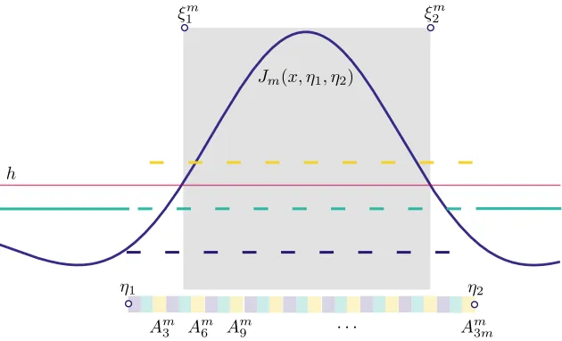
Fig. 7.Schematic of the analytical construction of a bump. A microscopic state whose partition comprises3m+ 2strips is considered. The microscopic state, which is not an equilibrium of the deterministic system, has a characteristic widthη2−η1, which differs from the widthξ2m−ξm1 of

the mesoscopic bumpJm. If we letm→ ∞while keepingη2−η1 constant, thenJmtends towards

a mesoscopic bumpJbandξmi →ηi(see Proposition5.1).

In the deterministic model, the transitions (2.5)–(2.7) are then replaced by the following rule

(4.2) u(x, t+ 1) =   

 

−1 ifx_∈X1(t),

0 ifx_∈X₋1(t)∪ X0(t)∩X<(t),

1 ifx_∈X0(t)∩X≥(t).

We stress that the right-hand side of the equation above depends onu(x, t), since the partitions_{X−1, X0, X1}and{X<, X≥} do so (see Remark2.1).

As we shall see, it is sometimes useful to refer to the induced mapping of the pullback sets

(4.3)

X−1(t+ 1) =X1(t)

X0(t+ 1) =X−1(t)∪ X0(t)∩X<(t)

X1(t+ 1) =X0(t)∩X≥(t)

.

Henceforth, we will use the termdeterministic model and formally write

(4.4) u(x, t+ 1) = Φd(u(x, t);γ).

for (4.2), where the partition _{Xk_}k∈Uis defined by (2.2) and the active and inactive

setsX_≥,X< by (4.1).

5. Macroscopic bump solution of the deterministic model. We now pro-ceed to construct a bump solution of the deterministic model presented in Section4. In order to do so, we consider a microscopic state with a regular structure, resulting in a partition, _{Xm

5.1. Bump construction. Starting from two points η1, η2 ∈ S, with η1 < η2,

we construct 3mintervals as follows

(5.1) Ami =

η1+i−1

3m (η2−η1), η1+ i

3m(η2−η1)

, i= 1, . . . ,3m, m∈N.

We then consider statesum(x) =P

k∈Uk1Xkm(x), with partitions given by

(5.2) Xm −1=

m [

j=1

Am

3j−2, X0m= [−L, η1)∪[η2, L)

m [

j=1

Am

3j−1, X1m=

m [

j=1

Am

3j, and activity set X≥ = [ξm1 , ξ2m]. We note that, in addition to the 3m strips that

form the active region of the bump, we also need two additional strips in the inactive region to form a partition ofS. In general,{ξim}i 6={ηi}i, as illustrated in Figure 7. Applying (4.2) or (4.3), we find Φd(um) 6= um, hence um are not equilibria of the

deterministic model. However, these states help us defining a macroscopic bump as a fixed point of a suitably defined map using the associated mesoscopic synaptic profile

(5.3) Jm(x, η1, η2) =κ

Z

Xm

1 (η1,η2)

W(x−y) dy,

where we have highlighted the dependence ofXm

1 onη1, η2. The proposition below

shows that there is a well defined limit,Jb, of the mesoscopic profile as m→ ∞. We

also have that ξmi → ηi as m→ ∞ and that the threshold crossings of the activity set are roots of a simple nonlinear function.

Proposition 5.1 (Bump construction). Let W be the periodic extension of the

synaptic kernel (2.1)and leth, κ_∈R+. Further, let{Aim}3i=1m,X1mandJmbe defined as in (5.1),(5.2)and (5.3), respectively, and letJb:S3→Rbe defined as

Jb(x, η1, η2) =

κ 3

Z η2

η1

W(x₋y)dy.

The following results hold

1. Jm(x, η1, η2)→ Jb(x, η1, η2) as m → ∞ uniformly in the variable x for all

η1, η2∈S withη1< η2,

2. If there exists ∆∈(0, L)such that3h=κR∆

0 W(y)dy, then

Jb(0,0,∆) =Jb(∆,0,∆) =h.

Proof. We fix η1 < η2 and consider the 2L-periodic continuous mapping x 7→

Jb(x, η1, η2), defined onS. We aim to prove thatJm→Jbuniformly inS. We pose

I₋m1(x) =

m X

j=1

Z

A3j−2

W(x−y) dy,

Im

0 (x) =

m X

j=1

Z

A3j−1

W(x₋y) dy,

I1m(x) =

m X

j=1

Z

A3j

W(x₋y) dy,

for allx_∈S,m∈N. Since the intervals{Ami }3i=1m form a partition of [η1, η2) we have

(5.4) 3

κJb(x) =I m

−1(x) +I0m(x) +I1m(x) for allx∈S,m∈N.

Since W is continuous on the compact set S, it is also uniformly continuous on S. Hence, there exists a modulus of continuityω ofW:

ω(r) = sup p,q∈S

|p−q|≤r

|W(p)₋W(q)_|, with lim

r→0+ω(r) =ω(0) = 0.

We useωto estimate_|Im

1 (x)−I0m(x)| as follows: |I1m(x)−I0m(x)| ≤

m X j=1 Z

A3j

W(x₋y)dy₋ Z

A3j−1

W(x₋y)dy = m X j=1

Z η1+33mj(η2−η1)

η1+33jm−1(η2−η1)

W(x−y)dy−

Z η1+3j3−1m (η2−η1)

η1+33jm−2(η2−η1)

W(x−y)dy = m X j=1

Z η1+33mj(η2−η1)

η1+3₃j_m−1(η2−η1)

W(x₋y)₋W

x₋y+η2−η1 3m dy ≤ m X j=1

Z η1+33mj(η2−η1)

η1+3j3−1m (η2−η1)

W(x₋y)₋W

x₋y+η2−η1 3m dy ≤ m X j=1

Z η1+₃3_mj(η2−η1)

η1+3j3−1m (η2−η1)

ω _η

2−η1

3m

dy

=ω _η

2−η1

3m _η

2−η1

3 .

We have then |Im

1 (x)−I0m(x)| → 0 as m → ∞ and since ω (η2−η1)/(3m) is

independent ofx, the convergence is uniform. Applying a similar argument, we find

|Im

−1(x)−I0m(x)| → 0 asm → ∞ and using (5.4), we conclude I1m, I0m, I−m1 →Jb/κ

as m→ ∞. SinceI1m=Jm/κ, thenJm →Jb uniformly for all x∈Sand η1, η2 ∈S withη1< η2, that is, result 1 holds true.

By hypothesisJb(0,0,∆) =hand, using a change of variables under the integral

and the fact thatW is even, it can be shown thatJb(∆,0,∆) =h, which proves result

2.

Corollary 5.2 (Bump symmetries). Let ∆ be defined as in Proposition 5.1,

thenJb(x+δ, δ, δ+ ∆) is a mesoscopic bump for allδ∈[L,−∆ +L). Such bump is symmetric with respect to the axisx=δ+ ∆/2.

Proof. The assertion is obtained using a change of variables in the integral defining Jb and noting thatW is even.

The results above show that,ξm

i →ηi as m→ ∞, hence we lose the distinction between width of the microscopic pattern, η2 −η1, and width of the mesoscopic

pattern, ξm

2 −ξm1 , in that result 2 establishes Jb(ηi, η1, η2) = h, for η1 = 0, η2 =

∆. With reference to Figure 7, the factor 1/3 appearing in the expression for Jb

confirms that, in the limit of infinitely many strips, only a third of the intervals

{Amj }jcontribute to the integral. In addition, the formula forJbis useful for practical

computations as it allows us to determine the width, ∆, of the bump.

Remark 5.3 (Permuting intervals Ami ). A bump can also be found if the

par-tition _{Xm

Proposition 5.1 can be extended to a more general case of permuted intervals. More precisely, if we consider permutations, σj, of the index sets _{3j₋2,3j₋1,3j_} for

j= 1, . . . , m and construct partitions

X₋m1=

m [

j=1

Amσj(3j−2), X m

0 = [−L,0)∪[∆, L)

m [

j=1

Amσj(3j−1), X m

1 =

m [

j=1

Amσj(3j),

then the resultingJm converges uniformly toJb as m→ ∞. The proof of this result follows closely the one of Proposition5.1 and is omitted here for simplicity.

5.2. Bump stability. Once a bump has been constructed, its stability can be studied by employing standard techniques used to analyse neural field models [11]. We consider the map

Ψb:S2×S2→R2, (ξ, η)7→

Jb(ξ1, η1, η2)−h

Jb(ξ2, η1, η2)−h

.

and study the implicit evolution

(5.5) Ψb(ξ(t+ 1), ξ(t)) = 0.

The motivation for studying this evolution comes from Proposition 5.1, according to which the macroscopic bump ξ∗ = (0,∆) is an equilibrium of (5.5), that is, Ψb(ξ∗, ξ∗) = 0. To determine coarse linear stability, we study how small pertur-bations ofξ∗ evolve according to the implicit rule (5.5). We setξ(t) =ξ∗+εξ(t), fore 0 < 1 with ξie = O(1) and expand (5.5) around (ξ_∗, ξ_∗), retaining terms up to orderε,

Ψb(ξ∗+εξ(te + 1), ξ_∗+εξ(t)) = Ψe b(ξ∗, ξ∗) +εDξΨb(ξ∗, ξ∗)ξ(te + 1) +εDξΨb(ξ∗, ξ∗)ξ(t).e Using the classical ansatz ˜ξ(t) =λt_{v, withλ}

∈Candv∈S2, we obtain the eigenvalue problem

(5.6) λ

v1

v2

= 1

W(0)−W(∆)

−W(0) W(∆) W(∆) ₋W(0)

v1

v2

,

with eigenvalues and eigenvectors given by

λ1=

W(∆)₋W(0)

W(0)₋W(∆) =−1, v

1_{= (1,1)}T_,

λ2=−

W(0)₋W(∆)

W(0)−W(∆) , v

2_{= (}

−1,1)T_.

As expected, we find an eigenvalue with absolute value equal to 1, corresponding to a pure translational eigenvector. The remaining eigenvalue, corresponding to a compression/extension eigenvector, determines the stability of the macroscopic bump. The parametersAi,Bi in Equation (2.1) are such thatW has a global maximum at x= 0, withW(0)>0. Hence, the eigenvalues are finite real numbers and the pattern is stable ifW(∆)<0. We will present concrete bump computations in Section 10.

4

2

⇡ _ξ1 ξ2 0 ⇠3 ⇠4 ⇡

v2 v1 v3 v4 x J

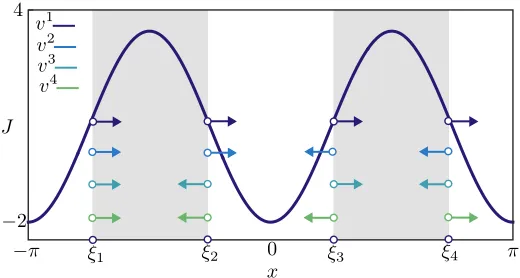
Fig. 8. Stable mesoscopic multi-bump obtained for the deterministic model. We also plot the corresponding macroscopic bumpξ∗ (Equations (5.7)–(5.8)) and coarse eigenvectors. Parameters

areκ= 30,h= 0.9,p= 1,β→ ∞, with other parameters as in Table1

5.3. Multi-bump solutions. The discussion in the previous section can be extended to the case of solutions featuring multiple bumps. For simplicity, we will discuss here solutions with 2 bumps, but the case ofkbumps follows straightforwardly. The starting point is a microscopic structure similar to (5.2), with two disjoint inter-vals [η1, η2),[η3, η4) ⊂S each subdivided into 3m subintervals. We form the vector η={ηi}4

i=1 and have

κ Z

Xm

1

W(x−y)dy=

2

X

j=1

Jm(x, η2j−1, η2j)→ 2

X

j=1

Jb(x, η2j−1, η2j),

asm_{→ ∞}uniformly in the variablexfor allη1, . . . , η4∈Swithη1< . . . < η4. In the

expression above,JmandJbare the same functions used in Section5.1for the single

bump. In analogy with what was done for the single bump, we consider the mapping defined by

Ψ : S4×S4→R4, (ξ, η)7→

−h+

2

X

j=1

Jb(ξi, η2j−1, η2j)

4 i=1

.

Multi-bump solutions can then be studied as in Section 5. We present here the results for a multi-bump forL=πwith threshold crossings given by

(5.7) ξ∗=

1 2    

−π−∆

−π+ ∆ π₋∆ π+ ∆



   ,

where ∆ satisfies

(5.8) Jb

π+ ∆

2 ,

−π−∆

2 ,

−π+ ∆ 2

+Jb

π+ ∆

2 , π−∆

2 , π+ ∆

2

=h.

A quick calculation leads to the eigenvalue problem

(5.9) λ     v1 v2 v3 v4     = 1 α    

W(0) −W(∆) W(π) −W(π−∆)

−W(∆) W(0) −W(π−∆) W(π)

W(π) ₋W(π₋∆) W(0) ₋W(∆)

where α = ₋W(0) +W(∆)₋W(π) +W(π₋∆). The real symmetric matrix in Equation (5.9) has eigenvalues and eigenvectors given by

λ1= −W(0) +W(∆)−W(π) +W(π−∆)

W(0)₋W(∆) +W(π)₋W(π₋∆) =−1, v

1_{= (1,1,1,1)}T_,

λ2= −

W(0) +W(∆) +W(π)₋W(π₋∆)

W(0)₋W(∆) +W(π)₋W(π₋∆) , v

2_{= (1,1,}

−1,₋1)T,

λ3= −

W(0)₋W(∆)₋W(π)₋W(π₋∆)

W(0)−W(∆) +W(π)−W(π−∆) , v

3_{= (1,}

−1,1,₋1)T,

λ4= −

W(0)₋W(∆) +W(π) +W(π₋∆)

W(0)−W(∆) +W(π)−W(π−∆) , v

4_{= (1,}

−1,−1,1)T.

As expected, we have one neutral translational mode. If the remaining 3 eigenvalues lie in the unit circle, the multi-bump solution is stable. A depiction of this multi-bump, with corresponding eigenmodes can be found in Figure8. We remark that the multi-bump presented here was constructed imposing particular symmetries (the pattern is even; bumps all have the same widths). The system may in principle support more generic bumps, but their construction and stability analysis can be carried out in a similar fashion.

6. Travelling waves in the deterministic model. Travelling waves in the deterministic model can also be studied via threshold crossings, and we perform this study in the present section. We seek a measurable function utw: S → U and a constantc_∈Rsuch that

(6.1) u(x, t) =utw(x−ct) =

X

k∈U

k1Xtw

k (x−ct)

almost everywhere inS and for allt∈Z. We recall that, in general, a stateu(x, t) is completely defined by its partition,{Xtw

k (t)}. Consequently, Equation (6.1) expresses that a travelling wave has a fixed profileutw, whose partition,{Xktw}, does not depend on time. A travelling wave (utw, c) satisfies almost everywhere the condition

utw=σ−cΦd(utw;γ),

where Φdis the deterministic evolution operator (4.4) and the shift operator is defined

by σx: u(_·) _7→ u(_{· −}x). The existence of a travelling wave is now an immediate consequence of the symmetries of W, as shown in the following proposition. An important difference with respect to the bump is that analytical expressions can be found for both microscopic and mesoscopic profiles, as opposed to Proposition 5.1, which concerns only the mesoscopic profile.

Proposition 6.1 (Travelling wave). Let h, κ ∈R+. If there exists ∆ ∈ (0, L) such that h=κR2∆

∆ W(y)dy, then

utw(z) =

X

k∈U

k1Xtw

k (z), with partition

X₋tw1= [−2∆,−∆),

X0tw= [−L,−2∆)∪[0, L),

X1tw= [−∆,0),

is a travelling wave of the deterministic model (4.4) with speed c = ∆, associated mesoscopic profileJtw(z) =κR

0

−∆W(z−y) dy and activity setX tw

≥ = [−2∆,∆].

(b) (a)

t= 1

t= 30

t= 49

0.03 0.004

0.003

0.01 0.01

σ−t∆Φd(utw+ε˜u), κ= 38 σ−t∆Φd(utw+ε˜u), κ= 33

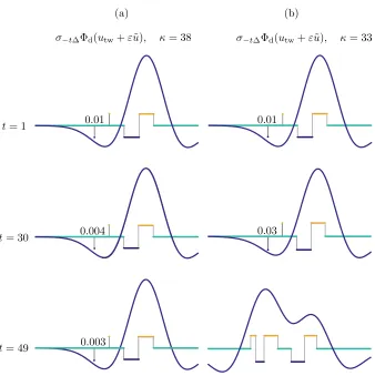
Fig. 9.Numerical investigation of the linear stability of the travelling wave of the deterministic

system, subject to perturbations in the wake of the wave. We iterate the map Φd starting from a

perturbed stateutw+εu˜, whereutwis the mesoscopic wave profile of Proposition6.1, travelling with

speed∆, andεu˜ is non-zero only in two intervals of width0.01in the wake of the wave. We plot

σ−t∆Φd(utw+εu˜)and the corresponding macroscopic profile as a function oftand we annotate the

width of one of the perturbations. (a): Forκ= 38, the wave is stable. (b): for sufficiently smallκ, the wave becomes unstable.

Proof. The assertion can be verified directly. We have

h κ =

Z 2∆

∆

w(y)dy= Z 0

−∆

W(∆₋y)dy= Z 0

−∆

W(₋2∆₋y)dy,

hence the activity set forutwisX_≥tw= [−2∆,∆] with mesoscopic profileκR 0

−∆W(z−

y) dy. Consequently, Φd(utw;γ) has partition

Y₋1= [−∆,0),

Y0= [−L,−∆)∪[∆, L),

Y1= [0,∆],

andutw=σ−∆Φd(utw, γ) almost everywhere.

shown in Section 10. The main difference between utw and the stochastic waves

observed in Figure4 is in the wake of the wave, where the former features quiescent neurons and the latter a mixture of quiescent and refractory neurons.

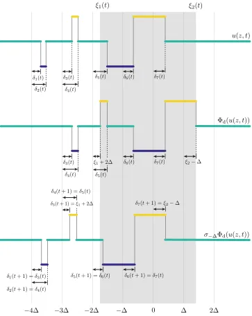
6.1. Travelling wave stability. As we will show in Section 10, waves can be found for sufficiently large values of the gain parameter κ. However, when this pa-rameter is below a critical value, we observe that waves destabilise at their tail. This type of instability is presented in the numerical experiment of Figure 9. Here, we iterate the dynamical system

(6.2) u(z, t+ 1) =σ−∆Φd(u(z, t)), u(z,0) =utw(z) +εu(z),e

whereutwis the profile of Proposition6.1, travelling with speed ∆, and the

perturba-tionεuetwis non-zero only in two intervals of width 0.01. We deem the travelling wave stable ifu(z, t)→utw(z) ast→ ∞. Forκsufficiently large, the perturbations decay,

as witnessed by their decreasing width in Figure9(a). Forκ= 33, the perturbations grow and the wave destabilises.

To analyse the behaviour of Figure9, we shall derive the evolution equation for a relevant class of perturbations toutw. This class may be regarded as a generalisation

of the perturbation applied in this figure and is sufficient to capture the instabilities observed in numerical simulations. We seek solutions to (6.2) with initial condition u(z, t) =P

kk1Xk(t)(z) with time-dependent partitions X₋1(t) =

h

−4∆ +δ1(t),−4∆ +δ2(t)

∪h−2∆ +δ5(t),−∆ +δ6(t)

,

X0(t) =

h

−L,₋4∆ +δ1(t)

∪h−4∆ +δ2(t),−3∆ +δ3(t)

∪h−3∆ +δ4(t),−2∆ +δ5(t)

∪hδ7(t), L

,

X1(t) =

h

−3∆ +δ3(t),−3∆ +δ4(t)

∪h−∆ +δ6(t), δ7(t)

,

and activity setX≥(t) = [ξ1(t), ξ2(t)]. In passing, we note that forδi= 0, the partition

above coincides with _{Xtw

k } in Proposition6.1, hence this partition can be used as perturbation ofutw. Inserting the ansatz for u(ξ, t) into (6.2), we obtain a nonlinear

implicit evolution equation, Ψ δ(t+ 1), δ(t)

= 0, for the vector δ(t) as follows (see Figure10)

δ1(t+ 1) =δ3(t)

δ2(t+ 1) =δ4(t)

Z −3∆+δ4(t) −3∆+δ3(t)

w(₋2∆ +δ3(t+ 1)−y)dy+

Z δ7(t) −∆+δ6(t)

w(₋2∆ +δ3(t+ 1)−y)dy=h/κ

δ4(t+ 1) =δ5(t)

δ5(t+ 1) =δ6(t)

δ6(t+ 1) =δ7(t)

Z −3∆+δ4(t) −3∆+δ3(t)

w(∆ +δ7(t+ 1)−y)dy+

Z δ7(t) −∆+δ6(t)

w(∆ +δ7(t+ 1)−y)dy=h/κ.

We note that the map above is valid under the assumption δ3(t)< δ4(t), which

preserve the number of intervals of the original partition. As in [44], we note that this

prevents us from looking at oscillatory evolution ofδ(t). We setδi(t) =ελt_{vi, retain} terms up to first order and obtain an eigenvalue problem for the matrix

1 α          

0 0 α 0 0 0 0

0 0 0 α 0 0 0

0 0 ₋w(∆) w(∆) 0 ₋w(∆) w(2∆)

0 0 0 0 α 0 0

0 0 0 0 0 α 0

0 0 0 0 0 0 α

0 0 w(4∆) ₋w(4∆) 0 w(2∆) ₋w(∆)           ,

where α = w(2∆)₋w(∆). Once again, we have an eigenvalue on the unit circle, corresponding to a neutrally stable translation mode. If all other eigenvalues are within the unit circle, then the wave is linearly stable. Concrete calculations will be presented in Section10.

7. Approximate probability mass functions for the Markov chain model.

We have thus far analysed coherent states of a deterministic limit of the Markov chain model, and we now move to the more challenging stochastic setting. More precisely, we return to the original model (2.8) and find approximate mass functions for the coherent structures presented in Section3 (see Figures2–4). These approximations will be used in the lifting procedure of the equation-free framework.

The stochastic model is a Markov chain whose 3N_-by-3N _{transition kernel has} entries specified by (2.1). It is useful to examine the evolution of the probability mass function for the state of a neuron at position xi in the network, µk(xi, t) = Pr u(xi, t) =k

,k_∈U, which evolves according to

(7.1) 



µ₋1(xi, t+ 1)

µ0(xi, t+ 1)

µ1(xi, t+ 1)



= 



1₋p 0 1

p 1₋f(J(u))(xi, t) 0 0 f(J(u))(xi, t) 0 

 



µ₋1(xi, t)

µ0(xi, t)

µ1(xi, t)



,

or in compact notationµ(xi, t+1) = Π(xi, t)µ(xi, t). We recall thatf is the sigmoidal firing rate and thatJ is a deterministic function of the random vector,u(x, t)∈UN, via the pullback setXu

1(t):

J(u)(x, t) =κ Z

X

W(x₋y)1Xu

1(t)(y) dy.

As a consequence, the evolution equation for µ(xi, t) is non-local, in that J(xi, t) depends on the microscopic state of the whole network.

We now introduce an approximate evolution equation, obtained by posing the problem on a continuum tissueSand by substitutingJ(x, t) by its expected value

(7.2) µ(x, t+ 1) =Π(x, t)µ(x, t),e

whereµ:S×Z→[0,1]3,

(7.3) Π(x, t) =e





1−p 0 1

p 1−f E[J](x, t) 0 0 f E[J](x, t) 0 

,

and

(7.4) E[J](x, t) =κ

Z

S

⇠1(t) ⇠2(t)

1(t)

2(t)

3(t)

4(t)

6(t) 7(t)

3(t)

4(t)

5(t)

6(t) 7(t) ⇠2

4 3 2 0 2

2(t+ 1) = 4(t) 1(t+ 1) = 3(t)

5(t) ⇠1+ 2

3(t+ 1) =⇠1+ 2 4(t+ 1) = 5(t)

5(t+ 1) = 6(t) 6(t+ 1) = 7(t) 7(t+ 1) =⇠2

u(z, t)

d(u(z, t))

d(u(z, t))

Fig. 10. Visualisation of one iteration of the system (6.2): a perturbed travelling wave (top) is first transformed by Φd using the rules (4.3) (centre) and then shifted back by an amount ∆

(bottom). This gives rise to an implicit evolution equationΨ δ(t+ 1), δ(t)

= 0 for the threshold crossing points of the perturbed wave, as detailed in the text.

In passing, we note that the evolution equation (7.2) is deterministic. We are inter-ested in two types of solutions to (7.2):

1. A time-independent bump solution, that is a mappingµbsuch thatµ(x, t) =

µb(x) for allx∈Sandt∈Z.

2. A travelling wave solution, that is, a mappingµtw and a real numberc such

7.1. Approximate probability mass function for bumps. We observe that, posingµ(y, t) =µb(y) in (7.2), we have

E[J](x) =κ Z

S

w(x₋y)(µb)1(y) dy,

Motivated by the simulations in Section3 and by Proposition5.1, we seek a solution to (7.2) in the limit β _{→ ∞}, with E[J](x)≥ hfor x∈[0,∆], and (µb)1(x)6= 0 for

x_∈[0,∆], where ∆ is unknown. We obtain

µb(x) =Πeb(x)µb(x),

where

e Πb(x) =





1−p 0 1

p 1 0

0 0 0



1_S\[0,∆](x) +





1−p 0 1

p 0 0

0 1 0



1[0,∆](x)

=Q<1S\[0,∆](x) +Q≥1[0,∆](x),

We conclude that, for eachx_∈[0,∆] (respectively x_∈S\[0,∆]),µb(x) is the right k·k1-unit eigenvector corresponding to the eigenvalue 1 of the stochastic matrix Q≥ (respectivelyQ<). We find

(7.5) µb(x) =



 0 1 0 

1_S\[0,∆](x) +

p 1 + 2p



 1/p

1 1



1[0,∆](x)

and, by imposing the threshold condition E[J](∆) = h, we obtain a compatibility condition for ∆,

(7.6) h= κp

1 + 2p Z ∆

0

w(∆−y) dy.

We note that if p= 1 we haveE[J](x) =Jb(x,0,∆) where Jb is the profile for the

mesoscopic bump found in Proposition5.1, as expected.

In Figure11(a), we plotµb(x) as predicted by (7.5)–(7.6), forp= 0.7, κ= 30, h=

0.9. At each x, we visualise (µb)k for each k ∈ U using vertically juxtaposed color bars, with height proportional to the values (µb)k, as shown in the legend. For a

qualitative comparison with direct simulations, we refer the reader to the microscopic profileu(x,50) shown in the right panel of Figure2(a): the comparison suggests that eachu(xi,50) is distributed according toµb(xi).

We also compared quantitatively the approximate distributionµb with the

dis-tribution, µ(x, t), obtained via Monte Carlo samples of the full system (7.1). The distributions are obtained from a long-time simulation of the stochastic model sup-porting a microscopic bumpu(x, t) fort_∈[0, T], withT = 105_{. At each discrete time}

t, we compute the mesoscopic profile, J(u)(x, t), the corresponding threshold cross-ings and width: ξ1(t),ξ2(t), ∆(t) and then produce histograms for the random profile

u(x₋ξ1(t)−∆(t)/2, t). The instantaneous shift applied to the profile is necessary to

pin the wandering bump.

0 0

1

2 _x 2 2 0 _x 2

µb µ1

µ0

µ-1 µ

(a) (b)

p= 1, ! 1 p= 0.7, = 5

(c) (d)

1 1.5 2 2.5 3 3.5 4

1 4

⇠Pr( )

1 1.5 2 2.5 3 3.5 4

1 4

⇠Pr( )

Fig. 11.Comparison between the probability mass functionµb, as computed by(7.5)-(7.6), and

the observed distribution µof the stochastic model. (a): We compute the vector(µb)k,k∈Uin each strip using(7.7)and visualise the distribution using vertically juxtaposed color bars, with height proportional to the values(µb)k, as shown in the legend. (b): A long simulation of the stochastic

model supporting a stochastic bumpu(x, t) for t∈ [0, T], where T = 105_{. At each time t > 10}

(allowing for initial transients to decay), we computeξ1(t),ξ2(t),∆(t)and then produce histograms

for the random profile u(x−ξ1(t)−∆(t)/2, t). (c): in the deterministic limit the value of ∆is

determined by (7.6), hence we have a Dirac distribution. (d): the distribution of∆obtained in the Markov chain model. Parameters are as in Table1.

the numerically computed ones, in which this transition is smoother. This discrep-ancy arises because ∆(t) oscillates around an average value ∆ predicted by (7.6); the approximate evolution equation (7.2) does not account for these oscillations. This is visible in the histograms of Figure 11(c)-(d), as well as in the direct numerical simulation6(a).

7.2. Approximate probability mass function for travelling waves. We now follow a similar strategy to approximate the probability mass function for trav-elling waves. We poseµ(x, t) =µtw(x−ct) in the expression forE[J], to obtain

κ Z

S

w(x₋y)(µtw)1(y−ct) dy=κ

Z

S

w(x₋ct₋y)(µtw)1(y) dy=E[J](x−ct). Proposition6.1provides us with a deterministic travelling wave with speedc= ∆. The parameter ∆ is also connected to the mesoscopic wave profile, which has threshold crossingsξ1 =−2∆ andξ2= ∆. Hence, we seek for a solution to (7.2) in the limit

β → ∞, withE[J](z)≥hforx∈[−2c, c], and (µtw)1(z)6= 0 forz ∈[−2c, c], where

c is unknown. For simplicity, we pose the problem on a large domain whose size is commensurate with c, that is S = cT /R, where T is an even integer much greater than 1.

We obtain

σctµtw(z) =Πetw(z−c(t−1))Πetw(z−c(t−2))· · ·Πetw(z)µtw(z),

where

e

Πtw(z) =Q<1S\[−c,c](z) +Q≥1[−2c,c](z).

To make further analytical progress, it is useful to partition the domainS=cT /R in strips of widthc,

S= T /2

[

j=T /2

jc,(j+ 1)c =

T /2−1

[

j=T /2

Ij(c),

and impose that the wave returns back to its original position after T iterations, σcTµtw(z) = µtw(z), while satisfying the compatibility condition h= E[J](c). This leads to the system

(7.7)

µtw(z) =R(z, c)µtw(z) =

" T /2−1

X

j=−T /2

Rj1Ij(c)(z) #

µtw(z),

κ Z c

−2c

W(c−y)(µtw)1(y) dy=h.

With reference to system (7.7) we note that:

1. R(z, c) is constant within each stripIj, hence the probability mass function, µtw(z), is also constant in each strip, that is, µtw(z) = P_iρi1Ii(c)(z) for some unknown vector (ρ₋T /2, . . . , ρT /2)∈S3T.

2. Each Rj is a product of T 3-by-3 stochastic matrices, each equal toQ< or Q≥. Furthermore, the matrices {Rj} are computable. For instance, for the stripI−1 we have

R₋1=



 

(1₋p)T _+p(1

−p)T−2 ₍₁

−p)T−2 ₍₁

−p)T−1

p(1₋p)T−1_+p2₍₁

−p)T−3 _p(1

−p)T−3 _p(1

−p)T−2

1₋(1₋p)T−1

−p(1₋p)T−3 ₁

−(1₋p)T−3 ₁

−(1₋p)T−2



 .

Consequently,µtw(z) can be determined by solving the following problem in the

un-known (ρ₋T /2, . . . , ρT /2, c)∈S3T ×R:

(7.8)

ρi−Riρi= 0, i=−T /2, . . . , T /2−1,

−h+κ(ρ₋1)1

Z 0

−c

W(c₋y) dy= 0.

Before presenting a quantitative comparison between the numerically determined distribution, µtw(z), and that obtained via direct time simulations, we make a few

efficiency considerations. In the following sections, it will become apparent that sam-pling the distribution µtw(z) for various values of control parameters, such as h or

(a) (b)

µ1

µ0

µ-1

4

0 0

4 4 4

0 1

µ µtw

I-1 I-1

z z

Fig. 12. Similarly to Figure 11, we compare the approximated probability mass functionµtw,

and the observed distributionµof the stochastic model. (a): the probability mass function is approx-imated using the numerical scheme outlined in the main text for the solution of (7.8); the stripI−1

is indicated for reference. (b): A set of9×105 _{realisations of the stochastic model for a travelling}

wave are run fort∈[0, T], whereT = 1000. For each realisations, we calculate the final thresh-old crossingsξs

1(T), ξ2s(T), and then compute histograms of us(x−ξ2s(T), T). We stress that the

strips in (a) are induced by our numerical procedure, while the ones in (b) emerge from the data. The agreement is excellent and is preserved across a vast region of parameter space (not shown). Parameters are as in Table1.

With little effort, however, we can obtain an accurate approximation to µtw,

with considerable computational savings. The inspiration comes once again from the analytical wave of Proposition 6.1. We notice that only the last equation of system (7.8) is nonlinear; the last equation is also the only one which couples _{ρj_} with c. When p = 1 the wave speed is known as β _{→ ∞}, N _{→ ∞} and p = 1 corresponds to the deterministic limit, hence E[J](z) =Jtw(z), which impliesc = ∆

and (ρ−1)1 = 1. The stochastic waves observed in direct simulations for p 6= 1,

however, displayc_≈(ξ2−ξ1)/3 = ∆ andµ≈1 in the strip whereJ achieves a local

maximum (see, for instance Figure4, for whichp= 0.4).

The considerations above lead us to the following scheme to approximateµtw: (i)

setc= ∆ and remove the last equation in (7.8); (ii) solveT decoupled 3-by-3 eigen-value problems to find ρi. Furthermore, if premains fixed in the coarse bifurcation analysis,ρi can be pre-computed and step (ii) can be skipped.

In Figure12(a), we report the approximateµtw found with the numerical

proce-dure described above. An inspection of the microscopic profile u(x,45) in the right panel of Figure 4(a) shows that this profile is compatible with µtw. We also

com-pared quantitatively the approximate distribution with the distribution, µ(x, t), ob-tained with Monte Carlo samples of the full system (7.1). The distributions are obtained fromM samples_{us_{(x, t)}

}M

s=1 of the stochastic model for a travelling wave

for t _∈ [0, T]. For each sample s, we compute the thresholds, ξs

1(T), ξ2s(T), of the

corresponding J(us_{)(x, T) and then produce histograms for u}s_(x−ξs

2(T), T). This

shifting, whose results are reported in Figure 12(b), does not enforce any constant value for the velocity, hence it allows us to test the numerical approximation µtw.

The agreement between the two distributions is excellent: we stress that, while the strips in Figure 12(a) are enforced by our approximation, the ones in Figure 12(b) emerge from the data. We note a slight discrepancy, in thatµtw(−3∆)≈0, while the

other distribution shows a small nonzero probability attributed to the firing state at ξ=₋3∆. Despite this minor disagreement, the differences between the approximated and observed distributions remain small across all parameter regimes of note and the

approximations even retain their accuracy asβ is decreased (not shown).

8. Coarse time-stepper. As mentioned in the introduction, equation-free meth-ods allow us to compute macroscopic states in cases in which a macroscopic evolution equation is not available in closed form [42, 43]. To understand the general idea be-hind the equation-free framework, we initially discuss an example taken from one of the previous sections, where an evolution equationdoes exist in closed form.

In Section 5, we described bumps in a deterministic limit of the Markov chain model. In this description, we singled out a microscopic state (the function um(x) with partition (5.2)) and a corresponding mesoscopic state (the function Jm(x)), both sketched in Figure 7. Proposition 5.1 shows that there exists a well defined mesoscopic limit profile, Jb, which is determined (up to translations in x) by its

threshold crossings ξ1 = 0, ξ2 = ∆. This suggests a characterisation of the bump

in terms of themacroscopic vector (ξ1, ξ2) or, once translation invariance is factored

out, in terms of themacroscopicbump width, ∆. Even though the microscopic state umis not an equilibrium of the deterministic system, the macroscopic state (0,∆) is a fixed point of the evolution equation (5.5), whose evolution operator Ψ is known in closed form, owing to Proposition 5.1. It is then possible to compute ∆ as a root of an explicitly available nonlinear equation.

We now aim to use equation-free methods to compute macroscopic equilibria in cases where we do not have an explicit evolution equation, but only a numerical pro-cedure to approximate Ψ. As mentioned in the introduction, the evolution equation is approximated using a coarse time-stepper, which maps the macroscopic state at timet0 to the macroscopic state at time t1 using three stages: lifting, evolution,

re-striction. The specification of these stages (the lifting in particular) typically requires some closure assumptions, which are enforced numerically. In our case, we use the analysis of the previous sections for this purpose. In the following section, we discuss the coarse time-stepper for bumps and travelling waves. The multi-bump case is a straightforward extension of the single bump case.

8.1. Coarse time-stepper for bumps. The macroscopic variables for the bump are the threshold crossings {ξi} of the mesoscopic profile J. The lifting op-erator for the bump takes as arguments{ξi}and returns a set of microscopic profiles compatible with these threshold crossings:

Lb:S2→UN×M, (ξ1, ξ2)T7→ {us(x)}s.

Ifβ _{→ ∞}, us_{(x) are samples of the analytical probability mass function µ}

b(x+

∆/2), where µb is given by (7.5) with ∆ =ξ2−ξ1. In this limit, a solution branch

may also be traced by plotting (7.6).

If β is finite, we either extract samples from the approximate probability mass functionµbused above, or we extract samplesus(x) satisfying the following properties

(see Proposition5.1and Remark 5.3):

1. us_{(x) is symmetric with respect to the axis x = (} e

ξ1+ξe2)/2, where ˜ξi =

round(ξi) and round :S→SN. 2. us_{(x) = 0 for allx∈[−L,}

e

ξ1)∪(ξe2, L).

3. The pullback sets, X1 andX−1, are contained within [ξe1,ξe2] and are unions

of a random number of intervals whose widths are also random. A schematic of the lifting operator for bumps is shown in Figure13.

l3

x l1

l2

d1= 1

d2= 1

l4

d4

d4

l4

l l4⇠Poisson(l)

d4⇠Bernoulli(d)

d

1 1

a 1 a

Fig. 13. Schematic representation of the lift operator for a bump solution. This figure displays a representation of how the states for neurons located within the activity set,[ξ1, ξ2], are lifted. For

illustrative purposes, we assume here that we are midway through the lifting operation, where 3 steps of thewhileloop listed in Algorithm1have been completed and a fourth one is being executed (shaded area). The widthl4 of the next strip is drawn from a Poisson distribution. The random

variable d ∈ {−1,1} indicates the direction through which we cycle through the states {−1,0,1}

during the lifting. The numberd4 is drawn from a Bernoulli distribution whose averageagives the

probablity of changing direction. For full details of the lifting operator, please refer to Algorithm1.

two possible examples of lifting. In our computations, we favour the second sampling method. The mesoscopic profiles,J, generated using this approach are well-matched toE[J] produced by the analytically derived probability mass functions (7.5). Numer-ical experiments demonstrate that this method is better than the first possible lifting choice at continuing unstable branches. This is most likely due to the fact that the latter method slightly overestimates the probability of neurons within the bump to be in the spiking state, and underestimates that of them being in the refractory state and this helps mitigate the problems encountered when finding unstable states caused by the combination of the finite size of the network and non-smooth characteristics of the model (whenβ is high).

The evolution operator is given by

ET: UN×M →UN×M, {uj(x)}j 7→ {ϕT(uj(x))}j,

whereϕT denotesT compositions of the microscopic evolution operator (2.8) and the dependence on the control parameter,γ, is omitted for simplicity.

For the restriction operator, we compute the average activity set of the profiles. More specifically, we set

R:UN×M →S2, {uj(x)}j7→(ξ1, ξ2)T,

where

ξi = 1 M

M X

s=1

ξis, i= 1,2,

and ξs

i are defined using a piecewise first-order interpolant PN3J of J with nodes

{xi_}N i=0,

ξs1=

x_∈S: PN3J(us)(x) =h, d dxP

3

NJ(us)(x)>0

,

ξs2=

x_∈S: PN3J(us)(x) =h, d dxP

3

NJ(us)(x)<0

.