Bayesian and Information-theoretic
Tools for Neuroscience
PhD Thesis
Dominik M. Endres
[email protected]
School of Psychology, University of St Andrews,
St Andrews KY16 9JP, U.K.
Abstract
The overarching purpose of the studies presented in this report is the exploration of the uses of information theory and Bayesian inference applied to neural codes. Two approaches were taken: Starting from first principles, a coding mechanism is proposed, the results are compared to a biological neural code. Secondly, tools from information theory are used to measure the information contained in a biological neural code.
Chapter 3: The REC model proposed by Harpur and Prager [33] codes inputs into a sparse, factorial representation, maintaining reconstruction accuracy. Here I propose a modification of the REC model to determine the optimal network dimen-sionality. The resulting code for unfiltered natural images is accurate, highly sparse and a large fraction of the code elements show localized features. Furthermore, I propose an activation algorithm for the network that is faster and more accurate than a gradient descent based activation method. Moreover, it is demonstrated that asymmetric noise promotes sparseness.
Chapter 4: A fast, exact alternative to Bayesian classification is introduced. Computational time is quadratic in both the number of observed data points and the number of degrees of freedom of the underlying model. As an example applica-tion, responses of single neurons from high-level visual cortex (area STSa) to rapid sequences of complex visual stimuli are analyzed.
Declarations
I, Dominik Endres, hereby certify that this thesis, which is approximately 30000 words in length, has been written by me, that it is the record of work carried out by me and that it has not been submitted in any previous application for a higher degree.
October 14, 2006 signature:
I was admitted as a part-time research student in Feb. 1998 and as a candidate for the degree of PhD in Feb. 1998; the higher study for which this is a record was carried out in the University of St Andrews between 1998 and 2004.
October 14, 2006 signature:
I hereby certify that the candidate has fulfilled the conditions of the Resolution and Regulations appropriate for the degree of PhD in the University of St Andrews and that the candidate is qualified to submit this thesis in application for that degree.
date: signature of supervisor:
In submitting this thesis to the University of St Andrews I understand that I am giving permission for it to be made available for use in accordance with the regula-tions of the University Library for the time being in force, subject to any copyright vested in the work not being affected thereby. I also understand that the title and abstract will be published, and that a copy of the work may be made and supplied to any bona fide library or research worker.
Contents
1 Introduction 5
1.1 Tools for neuroscience: information theory and Bayesian inference . . 5
1.2 An apology to the reader . . . 7
1.3 Publications . . . 7
1.4 Acknowledgments . . . 7
2 Methods 9 2.1 Notation . . . 9
2.2 Gradient descent . . . 10
2.3 Probability theory . . . 12
2.3.1 Cox’s axioms and Jayne’s Desiderata . . . 14
2.3.2 Bayesian Inference . . . 15
2.3.3 The limit of certainty: deductive and plausible reasoning . . . 16
2.3.4 Probability distributions and densities . . . 18
2.4 Information theory . . . 19
2.4.1 Joint, conditional and relative entropy . . . 21
2.4.2 Mutual information . . . 22
2.4.3 Differential entropy . . . 23
2.5 Bayesian methods . . . 25
2.5.1 Inferring model parameters . . . 25
2.5.2 Choosing the prior . . . 26
2.5.3 Kullback-Leibler divergence in Bayesian inference . . . 27
2.6 Approximation techniques . . . 30
2.6.4 Variational methods . . . 32
3 Occam’s razor for factorial codes 34 3.1 Introduction . . . 34
3.2 The network . . . 36
3.2.1 Activation algorithms . . . 39
3.2.2 Gradient descent with clipping . . . 39
3.2.3 Sequential updating . . . 40
3.2.4 Quadratic programming . . . 40
3.3 Learning . . . 42
3.4 Results . . . 44
3.4.1 Comparison of activation algorithms . . . 44
3.4.2 Pruning . . . 45
3.4.3 Overcompleteness . . . 47
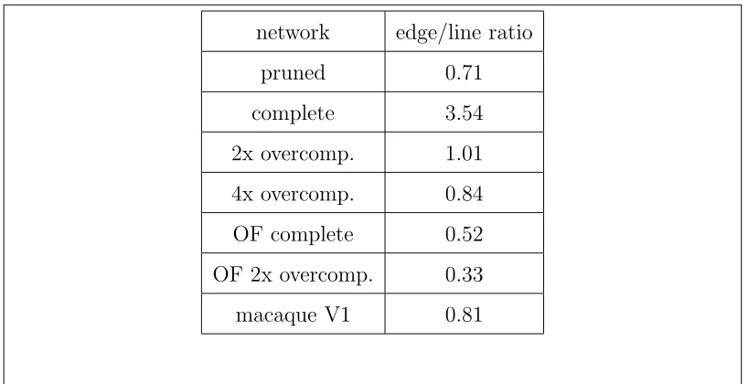
3.4.4 Quantitative comparison to V1 data and the generative model by Olshausen & Field . . . 52
3.5 Discussion . . . 60
3.5.1 The relationships between sparseness, overcompleteness, inde-pendence and redundancy reduction . . . 62
3.6 Asymmetric noise: a sparseness-promoting factor . . . 64
3.7 Conclusion . . . 68
4 Information extraction from neural spike trains I: Bayesian Bin Classification 70 4.1 Introduction . . . 70
4.2 Bayesian classification . . . 72
4.3 A simple model for P(y|w~) . . . 73
4.3.1 Why do the mapping f(w~)7→xfirst? . . . 74
4.3.2 A bin model for P(y|x) . . . 75
4.4 Computing p({{cj y}}|{zj}, M) . . . 78
4.5 Computing p({zj}|M) . . . 79
4.6 Computing the evidence . . . 79
4.7 Comparison to other classification methods . . . 82
4.8 Application to neural spike data . . . 86
4.8.1 Multiple datasets, joint and marginal expectations . . . 88
4.9 Results on artificial data . . . 88
4.10 RSVP results . . . 93
4.10.1 How similar are cells? . . . 93
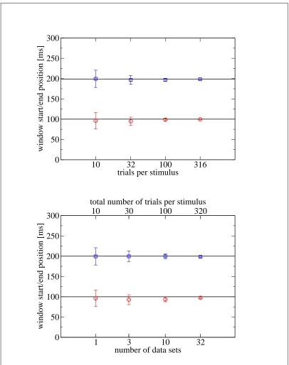
4.10.2 Latencies and response durations . . . 97
4.11 Conclusion . . . 99
4.11.1 Algorithm . . . 99
4.11.2 STSa neuron populations adapt their processing speed to the presentation rate . . . 100
5 Information extraction from neural spike trains II: Bayesian Bin Distribution Inference and Mutual Information 107 5.1 Introduction . . . 107
5.2 Bayesian binning . . . 109
5.3 Computing the prior p({(Pm, km)}|M) . . . 111
5.4 Computing the evidence . . . 112
5.5 Evaluating the model posterior P(M|D), the predictive distribution P(k|M, D) and its variance . . . 115
5.6 Inferring probability densities . . . 116
5.7 Model selection versus model averaging . . . 116
5.8 Computing the entropy and its variance . . . 118
5.8.1 Computing E[Pm′log(Pm′)|{km}, M, D] . . . 119
5.8.2 Computing E[Pm′log(∆km′)|{km}, M, D] . . . 120
5.8.3 Computing the variance . . . 121
5.8.4 Computing EPm2′log 2(P m′)|{km}, M, D . . . 122
5.8.5 Computing E[Pm′Pm′′log(Pm′) log(Pm′′)|{km}, M, D] . . . 122
5.9 An information-theoretic similarity measure . . . 123
5.10 Examples . . . 125
5.10.1 The limit K → ∞. . . 134
5.13 Sparse Priors . . . 142
5.13.1 Can (or should) finite-size effects be avoided? . . . 148
5.14 RSVP results . . . 150
5.14.1 Mutual information and information transmission rate . . . . 150
5.14.2 Temporal structure of the mutual information . . . 152
5.14.3 Is the mutual information zero? . . . 153
5.15 Conclusion . . . 156
5.15.1 Algorithm . . . 156
5.15.2 The information throughput of STSa neurons is maximized at SOA ≈ 60 ms . . . 158
6 Overall conclusion 160 Appendices 162 A Proof of minimum property 162 B Convergence of sequential updating 165 C Population decoding 170 D Dirichlet densities 172 D.1 Normalization Integral of a Dirichlet density . . . 172
D.2 Marginal densities . . . 174
D.3 Derivatives of Gamma and Beta functions . . . 174
D.4 An upper bound on the variance of a sum of random variables . . . . 178
D.5 Some identities for squares of sums . . . 179
E Proof of the metric properties of Dpq 180 E.1 Motivation . . . 180
E.2 Proof of metric properties of DPQ . . . 181
E.3 Asymptotic approximation . . . 184
E.4 Discussion . . . 184
Chapter 1
Introduction
We live in the information age: one can hardly look around and not see some device designed for the storage, transmission and processing of information. Computers in every office, TVs and radios at home, PDAs and pagers in many people’s pockets. In case one happens to forget this basic truth about modern life, the obnoxious ringtone of some mobile phone is guaranteed to remind him or her rather sooner than later.
Yet the most complex known information processing system, the one which helped to design and build the aforementioned ones, is still poorly understood: the human brain. The advancement of its understanding is the objective of neuroscience, which has gained tremendous momentum in the past few decades. Neuroscience is not limited to the study of the human brain: the nervous systems of other species are also under investigation.
1.1
Tools for neuroscience: information theory
and Bayesian inference
the purely descriptive to the study of its functional organization.
One of the aims of this thesis is to contribute to the understanding of the way in which the brain processes visual information. To that end, methods and princi-ples from two other disciplines will be employed: information theorymay loosely be defined as the mathematical study of information transmission and storage. Its fundamental concepts were developed by C. Shannon [83]. Probably his greatest contribution was the realization that information, properly defined, can be mea-sured. Consequently, he developed what he called the ’mathematical theory of communication’ [82]. Information theory will be used in two ways in this thesis:
1. In chapter 3, a (visual) coding scheme will be motivated by information-theoretic principles. The resulting codes turn out to be similar to those em-ployed by the early processing stages of the mammalian visual system. Fur-thermore, it will be demonstrated that the presence of noise in the information transmission process promotes sparse codes.
2. In chapter 5, a method will be developed for the information theoretic analysis of small and noisy datasets. As an example application, it will be applied to responses of neurons in area STSa (a high level visual cortex area) to complex visual stimuli.
Bayesian inference is the provably best way of reasoning in the presence of uncer-tain and incomplete information [54]. It is named after its founding father, Rev. T. Bayes [5], who pondered the question of how to determine whether a coin used for tossing is ’fair’, i.e. shows heads or tails with equal probability. After a long period of hibernation, it has enjoyed a revival in the last century [14, 43]. In this thesis, it will be used to develop an optimal method for information extraction from neural spike trains (more generally speaking, the algorithm presented in chapter 4 is an exact Bayesian classification scheme). Moreover, it is also an essential ingredient of the method for information theoretic response analysis (chapter 5).
1.2
An apology to the reader
I hope that the work presented in this thesis is found interesting by neuroscientists, and that the developed methods may be considered useful for future research. Since I am very hesitant to use a method which I do not fully understand, and assuming that the reader feels similarly, I placed heavy emphasis on explaining the methods in detail. The resulting presentational style may be deemed lengthy and ponderous by a pure mathematician. However, to the mathematically inclined neuroscientist, mathematics is a research tool, not an end in itself. Thus, many things which appear ’trivial’ and ’obvious’ to the former, may require explanation if to be understood by the latter without undue effort. In finding the right balance between brevity and clarity, I am heavily indebted to Peter F¨oldi´ak and Johannes Schindelin for their feedback. Most lengthier calculations and proofs have been relegated to various appendices.
1.3
Publications
The main findings of chapter 3 have been printed [20] and presented at theICANN’99
conference. Large parts of chapter 5 have appeared in the IEEE Transactions on Information Theory [22, 21]. The original work contained in these publications has for the most part been carried out by me, the co-authors contributed by posing the problems and, in the case of [22], by helping me with the correct mathematical formulation. We plan to publish another article focussing on the neuroscientific results obtained with the Bayesian Bin Distribution Inference method.
Moreover, a publication containing the theoretical development of chapter 4 and the resulting neuroscientific findings has been submitted.
1.4
Acknowledgments
develop my own ideas, always providing constructive criticism and pointing me in the right direction whenever I got stuck. I very much enjoyed his style of supervision, and sincerely hope that I did not overly strain his patience, when my theoretical investigations took me a little off course at times.
The neurophysiological recordings used in this thesis are a result of an earlier project by Christian Keysers, David Perret, Peter F¨oldi´ak and Dengke Xiao. I am grateful to D. Xiao and C. Keysers for supplying me with the data and explaining the formatting details to me. Furthermore, I’d like to thank D. Perret and Mike Oram for their feedback on my ideas and results. I would like to thank M. Oram for his constructive comments on my first-year report, too.
I also owe a debt of gratitude to Johannes Schindelin, with whom I enjoyed many stimulating discussions, who proofread drafts of this thesis and who helped me to clarify several notational issues.
Chapter 2
Methods
The research presented in this report was carried out using a variety of computational methods. In this chapter, the key concepts necessary to comprehend their working are outlined. For a more in-depth understanding, the reader is referred to the references given for each method. However, basic knowledge of linear algebra, one-dimensional calculus and probability theory are required.
2.1
Notation
Unless stated otherwise, the following notation will be used throughout this thesis:
• x, y, z denote real variables.
• ~x is a vector, whose components are real numbers.
• A is a M×N matrix.
• A,B,C are propositions, e.g. A=’A neuron in area STSa begins transmitting stimulus-related information 100 ms after the stimulus onset’.
• P(A|B) the conditional probability that proposition A is true given that propo-sition B is true.
• Logical operators: AB = A and B, A+B =A orB, ¯A = not A, A ⇒ B =
AimpliesB.
2.2
Gradient descent
A number of learning algorithms for artificial neural networks can be formulated as a minimization problem of a function of many variables (i.e. weights, biases etc.). In many cases, this function depends on its variables in a differentiable way. A necessary condition for a minimum of a differentiable function f(x) of one variable defined onIRis that it’s first derivative be zero atxmin, the point where the minimum
is located:
f′(xmin) =
df(x)
dx
x=xmin
= 0 (2.1)
If the function depends on more than one variable, the concept of the derivative needs to be suitably generalized for this condition to be applicable. This generalization is the gradient. The following derivation aims at making the idea plausible, a strict mathematical treatment can be found in [9].
Since the derivativef′(x0) is the incline of a tangent onf(x) atx0, the function
can be approximated by
f(x0+ ∆x)≈f(x0) + ∆f(x0) (2.2) where
∆f(x0) =f′(x0)∆x (2.3) This approximation (also known as a Taylor expansion to first order, see [9]) gets the better, the smaller ∆x.
Consider now a functiong(x1, x2, . . . , xN) ofN variables. Here, eqn. 2.2 becomes
g(x1+∆x1, x2+∆x2, . . . , xN+∆xN)≈g(x1, x2, . . . , xN)+∆g(x1, x2, . . . , xN) (2.4)
where
∆g(x1, x2, . . . , xN) = N
X
i=1
∂g(x1, x2, . . . , xN)
∂xi
∆xi (2.5)
∂g
∂xi is the partial derivative of g(x1, x2, . . . , xN) with respect to xi. It is computed
by the same rules as the derivative of a function of one variable, all variables xj, j ∈
{1,2, . . . , N} where j 6=i are treated as constants. Example: Let
g(x1, x2) =x21+x1x2+ 2x22 (2.6) Then
∂g(x1, x2)
∂x1
and
∂g(x1, x2)
∂x2
=x1+ 4x2 (2.8)
Lumping all the xi, ∆xi and ∂x∂g
i together in three vectors, ~x = (x1, x2, . . . , xN),
~
∆x = (∆x1,∆x2, . . . ,∆xN) and ~h = (
∂g(x1,x2,...,xN)
∂x1 ,
∂g(x1,x2,...,xN)
∂x2 , . . . ,
∂g(x1,x2,...,xN)
∂xN ),
eqn. 2.5 becomes
∆g(~x) =~h ~∆xT (2.9) i.e. ∆g(~x) is the inner product of~h and ∆~x. Now one could ask: Which vector ∆~x
gives rise to the greatest ∆g(~x)? Clearly, the longer ∆~x, the greater the absolute value of ∆g(~x). So instead, let’s try to find the ∆~x which produces the greatest ∆g(~x) amongst all possible ∆~x of equal length. Since the inner product of two vectors can also be expressed by their lengths and the angle between them, another form of eqn. 2.9 is
∆g(~x) =|~h||∆~x|cos(α) (2.10)
where α is the angle between |~h| and |∆~x|. As the length of ∆~x is fixed, ∆g(~x) will assume its maximum when the cosine of α is maximal, i.e. at α = 0. In other words, ∆g(~x) is maximal, if ∆~x is parallel to~h and oriented in the same direction. Moreover, ∆g(~x) is directly proportional to|~h|. Since eqn. 2.4 states that ∆g(~x) is the change ofg(~x) brought about by a small displacement given by∆~x, the direction of ~h tells us in which direction to go for maximal increase of g(~x), its length is a measure for the magnitude of this increase.
The vector~h is called the gradient of g(~x), it is usually denoted by
∇g(~x) = ∂g(~x)
∂~x = ( ∂g(~x)
∂x1
,∂g(~x) ∂x2
, . . . ,∂g(~x) ∂xN
) (2.11)
It shares (and generalizes) the following qualities with (of) the derivative f′(x) of a function f(x) of one variable:
1. ∇g(~x) points in the direction of the steepest incline of g(~x). In the one-dimensional case, there are only two directions: To the left and to the right. If f′(x) > 0, then f(x) increases when going to the right, if f′(x) < 0, it
decreases.
3. f′(x) = 0 is a necessary condition for an extremum of f(x). Similarly, when
∇g(~x) =~0, there is no direction (to first order) in which g(~x) increases at this point - which is a necessary condition for an extremum in a more-than-one dimensional space as well.
In order to find a minimum of g(~x), one could, starting from some point ~x0, follow the direction of the negative gradient (i.e. the direction of the steepest decline) until |∇g(~x)| = 0. This is the basic idea behind all gradient descent algorithms. In practice, however, it will be difficult to hit exactly the point where the gradient vanishes, because a step cannot be infinitesimally small, since then the algorithm would take infinitely long to reach the minimum. Hence, a downward step is usually taken to be proportional to the gradient (so that steps get smaller when the minimum is approached) and some step size parameter η (the ’learning rate’ in the neural networks community). The termination criterion is commonly of the form|∇g(~x)|< ǫ, where ǫ is some small positive constant. A typical implementation of a simple gradient descent algorithm would hence look somewhat like this:
1. Choose ~x0 (starting point), η (step size), and ǫ (termination threshold). 2. Set~x=~x0
3. Set∆~x=−η∇g(~x)
4. Set~x=~x+∆~x
5. if|∇g(~x)| ≥ǫ, goto step 3
6. Return ~x
Additionally, it is common to define a maximum number of steps after which the algorithm terminates, even if ǫ has not been reached.
2.3
Probability theory
propositions, it enables one to draw conclusions. However, in natural science, as op-posed to mathematics, one does seldom (if ever) have the luxury of certainty, which is necessary for its application. When conducting measurements, factors beyond the experimenter’s control will inevitably influence the results. What’s worse, these influences will usually not only be uncontrollable, they will also be unpredictable. Thus, another mode of reasoning is required, one that enables us to draw the best possible conclusions given the uncertitudes we have to contend with. This ’doctrine of chances’, as it was referred to by Rev. Thomas Bayes [5] almost 300 years ago, finds its modern counterpart in probability theory. Set down in axiomatic form by Kolmogorov [9], it has subsequently led to the accelerated development of statistics, which is considered indispensable for the analysis of experimental data.
While the axioms of probability (and thus, the theory deduced from them) stand largely undisputed, there has been quite a debate as to itsmeaning. Broadly speak-ing, there are two positions:
• Frequentist. Also known as ’sampling theory’, this approach views probabil-ity as the limit of relative frequency. Imagine the prototypical example: a coin is being tossed N times, and the number of times nh it shows ’heads’ upon
landing is recorded. The relative frequency of ’heads’ is then fh = nNh. By
virtue of the weak law of large numbers [9],fh converges in probability toPh,
the probability of ’heads’, if N → ∞:
lim
N→∞P(|fh−Ph| < ǫ) = 1 (2.12)
whereǫis some arbitrarily small positive number. Tossing the coin constitutes a ’random experiment’, which avails one of a sample drawn from the proba-bility distribution (Ph, Pt) (i.e. the probabilities of observing heads or tails,
respectively). Hence the name ’sampling theory’. The outcome of a toss is an instance of a random variable. In the frequentist perspective, probabilities can only be assigned to random variables.
key-random variables. They can be assigned to hypotheses as well, such as ’The coin is biased in favor of heads’ or ’A neuron in area STSa begins to transmit stimulus-related information 100 ms after the stimulus onset’. This does not imply that the truth or falsehood of the proposition in question is subject to random fluctuations, it only aims at quantifying the (subjective) uncer-tainty associated with the veracity of a statement due to a lack of information. The rules of probability theory can then be used to compute the plausibilities of logical compositions of such statements, and, most importantly, how the probabilities change when new data become available. This process is called
Bayesian inference.
2.3.1
Cox’s axioms and Jayne’s Desiderata
The proof that degrees of belief (or plausibility) can be described by probabilities was given in [14]. If one is willing to accept the Cox axioms (see e.g. [54]), then one is also forced to accept probability theory as the ’grammar’ of plausible reasoning. Instead of listing these axioms here, it is perhaps more instructive to consider the basic desiderata of plausible reasoning as presented in [43]:
1. Degrees of plausibility are represented by real numbers.
2. Qualitative correspondence with common sense.
3. (a) If a conclusion can be reasoned out in more than one way, then every possible way must lead to the same result.
(b) All of the available evidence relevant to a question is taken into account.
(c) Equivalent states of knowledge are represented by equivalent plausibility assignments.
Desideratum 1 could in principle be replaced by the weaker requirement of a total order, i.e. that the plausibility assignments (=probabilities) to any two propositions can be compared [43], but the resulting theory would then be less manageable in practice. Desiderata 2, 3a and 3c give rise to the sum an product rules for probability. Suppose we had 3 propositions A, B and C. Then
1 = P(A|C) +P( ¯A|C) (2.14)
0 ≤ P(A|C)≤1 (2.15)
Those rules are all that is needed to conduct inference. It is easy to show that
P(A|C) = 1 if A is true with certainty, and likewise that P(A|C) = 0 if A is false with certainty. Furthermore, if A does not depend on B, i.e. P(A|BC) =P(A|C), thenP(AB|C) = P(A|C)P(B|C). In this case, A and B are said to be independent. Proposition C stands for the evidence (desideratum 3b) relevant for the determina-tion of P(A|C) etc.. It is important to note that all probability assignments are based on such prior information, at least in the Bayesian view. This is the reason why, for the better part of the last century, many mathematicians and scientists have rejected the Bayesian perspective as ’subjective’, and, as a remedy, the fre-quentist interpretation of probability was claimed to be the only valid one, because it was deemed to be more objective. However, as argued in [52], this undertaking has largely failed. What scientists are usually interested in is assessing the proba-bility of various hypotheses, given a set of observed data. And it is precisely this kind of question which the frequentist approach cannot answer, because, by its very definition, probabilities can not be assigned to hypotheses.
In the author’s opinion, the basic desiderata are sufficiently compelling to justify the use of probability theory for inference in science. Moreover, since it was proven in [14] that any other set of rules would lead to a violation of the Cox axioms, and thus be in contradiction with these desiderata, it follows that probability theory is the only suitable tool for conducting inference.
2.3.2
Bayesian Inference
The original objective of Bayesian Inference, in the words of Rev. T. Bayes [5], is
”Given the number of times ion which an unknown event has happende and failed:
In other words, given the observed frequencies, what are the corresponding proba-bilities? This is an instance of a more general class of problems, namely: given a set of data, how plausible is some hypothesis? Those questions can be answered using probability theory. From the product rule (eqn. 2.13) follows
P(A|BC) = P(B|AC)P(A|C)
P(B|C) (2.16)
which is know as Bayes’ rule or Bayes’ theorem. Sometimes it is also referred to as the law of inverse probability, because it states howP(A|BC) is to be converted into
P(B|AC). Now suppose that B is a statement about a measurement of some kind, and A is a proposition which has a logical connection to B, e.g. a possible cause of B, or something that frequently coincides with B for reasons unknown. Information of this kind, represented in C, is called prior information. Moreover, C must allow for the assessment the probability ofA before observing B. Thus,P(A|C) is called the
prior probability of A, or just theprior. P(B|AC) is also needed, since it quantifies how likely B is deemed given A and C, it is referred to as the likelihood. P(B|C) could either be a part of the prior information as well, or, more customary, P(B|AC¯ ) is known. It is then possible to evaluate P(B|C) via eqn. (2.14):
P(B|C) = P((A+ ¯A)B|C) =P(AB|C) +P( ¯AB|C) = P(B|AC)P(A|C) +P(B|AC¯ )P( ¯A|C)
= P(B|AC)P(A|C) +P(B|AC¯ )(1−P(A|C)) (2.17)
P(B|C) is called the evidence of the data. The reasons for this name will become clear later. P(A|BC) is theposterior probability of A, so named because it tells how probable A becomes once the veracity of B has been established.
Bayesian Inference – for the most part – boils down to nothing more than the inversion of a conditioning via eqn. (2.16).
2.3.3
The limit of certainty: deductive and plausible
rea-soning
A ⇒ B A=true B=true
Translated into probabilities, the implication becomes
1 = P(AB¯|C) = 1−P(AB¯|C)
= 1−P( ¯B|AC)P(A|C) = 1−(1−P(B|AC))P(A|C)
⇒ P(B|AC) = 1
i.e. B is true with certainty as soon as A is observed to be true. As an example of plausible reasoning, the weak syllogism, which is a mode of reasoning often employed in science for the purpose of hypothesis generation
A ⇒ B B=true
A becomes more plausible
can be expressed as
1 = P(AB¯|C)
⇒0 = P(AB¯|C)
= P( ¯B|AC)P(A|C) = (1−P(B|AC))P(A|C) =
1−P(BA|C)
P(A|C)
P(A|C)
=
1−P(A|BC)P(B|C)
P(A|C)
P(A|C) = P(A|C)−P(A|BC)P(B|C)
⇒P(A|BC) = P(A|C)
P(B|C) | {z }
≤1
≥P(A|C) (2.18)
true: in that case P(B|C) = 1, and nothing is gained by observing B. This process of updating probabilities after observing data is referred to as Bayesian learning. Note also that eqn. (2.18) implies that C must be such that P(A|C)≤P(B|C). In other words, if one believes firmly in the validity of an implicationA⇒B, then one must also be sure that A is less likely than, or at most as likely as, B a priori. This corresponds to the common-sensical notion that A is one of the reasons which can lead to B, but not the only conceivable one. More on the correspondences between probability theory and classical logic can be found in [43].
2.3.4
Probability distributions and densities
The concept of random variables, so central to the frequentist approach, can be incorporated quite naturally into the Bayesian perspective. For the purposes of this thesis, the added generality of a measure-theroetic approach to probability offers little benefit. Thus, the following definitions will suffice:
• Discrete random variable. X is a discrete random variable, if it can take on countably many values xi. Each xi can be assumed with
probabil-ity P(X = xi|C). P(X = xi|C) is the probability distribution of X, which
has the properties
– ∀xi :P(X =xi|C)≥ 0
– P{xi}P(X =xi|C) = 1
• Continuous random variable. X is a continuous random variable, if every instance of X ∈ IR. X is distributed according to p(x|C), the probability density of X, which has the properties
– P(X∈[x, x+dx]|C) =p(x|C)dx
– ∀x∈IR:p(x|C)≥0
– R−∞∞ p(x|C)dx= 1
As before, C is the prior information on which the probability assignments are based. X =xiis just another statement, namely ’X takes on the valuexi’. Therefore,
condition P{x
i}P(X = xi|C) = 1 can be derived from the sum and product rules
on the condition that the statements are mutually exclusive, which is obviously a sensible requirement – X cannot take on more than one value at once. The usual shorthand for P(X =xi|C) is P(xi), where prior information C on which the
probability assessments are based is implicitly assumed. It will be used whenever unequivocally possible.
The generalization to a real-valued random variable is also straightforward and requires little comment. The density must be integrable (let’s say in the Riemannian sense [9], even though that is not the most general possible condition). What should perhaps be noted is that a further generalization to random variables which are vectors of real numbers is easily accomplished by replacing every occurrence of x
with ~x. Consequently, the normalization integral would then have to extend over
IRm, where m is the dimensionality of~x.
2.4
Information theory
Information theory is concerned with the theoretical aspects of information trans-mission, storage and, to some (small) extent, processing. This discipline was founded by C. Shannon [83], who also addressed and solved its most fundamental problems. Since the brain is an information processing system, it is natural to try to apply information theoretic principles and results in order to understand its functions. The following short overview will be phrased in terms of random variables, but the reader should keep in mind that each of those could be replaced by a set of mutually exclusive propositions.
The most central information theoretic quantity is entropy. In [82], it is argued that a general measure H of uncertainty of a random variable, whose probability distribution P(xi) = Pi, i = 1, . . . , N is assumed to be known , should fulfill the
following conditions:
1. H should be a continuous function of the Pi, i.e. if the probabilities change
of N. When uncertainty is understood as the number of questions one has to ask about X before its exact value is determined, then this number should grow with the number of possibilities.
3. H should not depend on the specific set of questions asked. Imagine sequences of questions were constructed that successively narrowed down the possible values of a given instance of X. The final determination of X must be the same for all such sequences. As an example, suppose N = 3. Then a possible first question would be ’is X =x1?’. Having received the answer ’yes’ (which would happen with probabilityP1), no more information would be needed. If, however, the answer was ’no’ (with probability 1−P1), then a second question would be in order, e.g. ’is X =x2?’. Thus, it is required of H that
H(P1, P2, P3) = H(P1,1−P1)
| {z }
1st question
+(1−P1)H( P2 1−P1
, P3
1−P2 )
| {z }
2nd question
(2.19)
This property is also called ’grouping’ [13].
It can be proven [82] that the only form of H compatible with these conditions is
H({Pi}) =−K N
X
i=1
Pilog(Pi) (2.20)
where K is some positive constant that determines the units of H. Alternatively,K
can be included in the logarithm via a change of basis
Klog(x) = logexp(1
K)(x) (2.21)
Common choices for the basis are:
• 2, in which case H is measured in bit. A bit is one ’yes/no’ information.
• e, the basis of the natural logarithm. The unit is then nats. 1 bit ≈ 0.6931 nats.
Since 0≤Pi ≤1, and limx−>0+xlog(x) = 0, it is apparent thatH ≥0 with equality
if there is no uncertainty about X. It is customary to denote the entropy by the random variable, not the probability distribution, i.e.
H({Pi}) =H(X) (2.22)
An important property of H is its relationship with codelength. It can be shown [13] that the minimum expected number of ’yes/no’ (i.e. binary) questions which need to be answered to determine X is between H(X) and H(X) + 1, when the latter is measured in bit. Since entropy can be written as an expectation as well
H(X) = −E[log(P(x))] (2.23)
it follows that,
−log2(P(xi)) (2.24)
is the number of bits needed to encode the message X = xi. In the terminology
of information theory, each xi is a symbol or code element. The set of all symbols
comprises the alphabet used for message encoding.
2.4.1
Joint, conditional and relative entropy
If a probability distribution is defined for two random variables X and Y, the joint entropy is given by
H(X, Y) =−X
xi
X
yj
P(xi, yj) log(P(xi, yj)) (2.25)
If X and Y are independent, then
H(X, Y) = −X
xi
X
yj
P(xi)P(yj) (log(P(xi)) + log(P(yj)))
= H(X) +H(Y) (2.26)
Likewise, the conditional entropy is
H(X|Y) =−X
xi
X
yj
P(xi, yj) log(P(xi|yj)) (2.27)
Another important quantity isrelative entropy or Kullback-Leibler divergence. Sup-pose we had two probability distributions P(x) and Q(x) for the same random vari-able, then
D(P(x)||Q(x)) = XP(x) log
P(xi)
It can be shown that (e.g. via Jensen’s inequality [13])
D(P(x)||Q(x))≥0 (2.29)
with equality if and only if P(x) = Q(x) for all possible x. This is known as Gibbs’ inequality [54], and it is one of the most central inequalities in information theory.
D(P(x)||Q(x)) can thus be seen as measure for how much P(x) deviates fromQ(x). Kullback-Leibler divergence has a number of interpretations, perhaps the most com-mon one being that of coding inefficiency: given a random variable is distributed ac-cording toP(x), it is possible to construct a code with average codelengthH(P(x)). If instead a code optimized forQ(x) was used, then the expected codelength would be−PxiPilog(Qi). Thus, the inefficiency – the superfluous codelength due to using
a suboptimal code – is
−X
xi
Pilog(Qi)− −
X
xi
Pilog(Pi)
!
=D(P(x)||Q(x)) (2.30)
Note that D(P(x)||Q(x)) will diverge whenever Qi = 0 and Pi 6= 0. This indicates
that the optimal code for X under Q(x) is not only suboptimal, but actually un-suitable for representing X underP(x): impossible values of X under Q(x) (Qi = 0)
would not need to be coded. If those values are possible under P(x), then a new coding scheme is definitely necessary.
2.4.2
Mutual information
Mutual information is defined as
I(X;Y) = X
xi
X
yj
P(xi, yj) log
P(xi, yj)
P(xi)P(yi)
(2.31)
where P(xi) = PyjP(xi, yi) and likewise for P(yj). Since it can be written as
I(X;Y) =D(P(xi, yj)||P(xi)P(yi)), it follows that
I(X;Y)≥0 (2.32)
with equality if and only if P(xi, yj) = P(xi)P(yi) for all xi and yi [13]. Another
way of expressing it is
I(X;Y) = X
xi
X
yi
P(xi, yi) log(
1
P(xi)
) +X
xi
X
yj
P(xi, yj) log
P(xi, yj)
P(yi)
= −X
xi
P(xi) log(P(xi)) +
X
xi
X
yj
P(xi, yj) log(P(xi|yi))
= H(X)−H(X|Y) (2.33)
i.e. the difference between the uncertainties about X before and after observing Y. Thus, it quantifies the reduction in uncertainty due to the knowledge of Y, or, in other words, it measures how much can be learnt about one random variable given another. For symmetry reasons, eqn. (2.33) could also have been written as
I(X;Y) =H(Y)−H(Y|X), whence the adjective ’mutual’.
For given H(X), I(X;Y) assumes a maximum when H(X|Y) = 0, i.e. when X is a function of Y. In this case (which also includes the identity function X =
Y), I(X;Y) = H(X). This opens up another perspective on entropy: instead of interpreting it as uncertainty, it can also be seen as the maximum amount of information that can be gained about a random variable (i.e. everything that is not already encoded in its probability distribution). Thus, entropy is sometimes called
self-information of X.
Mutual information is an important quantity in neuroscience. In this thesis, it will be employed to assess the information which a neural response carries about a visually presented stimulus.
2.4.3
Differential entropy
The concept of entropy can be generalized to continuous random variables, if some care is taken [13]. Since entropy measures the average amount of information re-quired to specify an instance of a random variable exactly, it will in general be ∞ if the random variable can take on infinitely many values. To see how this problem arises, assume a continuous random variable X was distributed according to the density p(x). Also, suppose that one could measure this variable with an accuracy ∆x across the whole (finite) domain ofX. The probability Pi of observing X in an
interval of width ∆x centered around xi is then Pi = ˜p(xi)∆x, where ˜p(xi) is the
mean density in this interval. The entropy of the observations xi thus obtainable
would then be given by (note that PiPi = 1, i.e. the intervals are assumed to be
non-overlapping):
= −X
i
˜
p(xi)∆xlog(˜p(xi)∆x) (2.35)
= −X
i
˜
p(xi)∆xlog(˜p(xi))−log(∆x) (2.36)
Let us now consider the limiting case of exact observations, i.e. the limit ∆x →0:
lim
∆x→0H(X) =− Z
dx p(x) log(p(x))−log(∆x) | {z }
−∞
=∞ (2.37)
where the integration extends over the domain ofX. Thus, the entropy will diverge, which indicates that knowing a continuous quantityexactly requires generally an in-finite amount of information. This is highlighted by the fact that the diverging term describes the measurement accuracy ∆x. Therefore, it is not possible to define the entropy of a continuous random variable. However, it is possible to measure the dif-ference between entropies of continuous variables under certain conditions: assume a second random variableY was distributed according top(y), and measurable with the same accuracy as X, ∆x. Then
H(X)−H(Y) = −X
i
˜
p(xi)∆xlog(˜p(xi))−log(∆x)
+X
i
˜
p(yi)∆xlog(˜p(yi)) + log(∆x)
= X
i
˜
p(xi)∆xlog(˜p(xi)) +
X
i
˜
p(yi)∆xlog(˜p(yi)) (2.38)
Taking the limit ∆x → 0 might now very well be possible, because the diverging term in eqn. (2.37) has cancelled out. Thus, thedifferential entropy ofX ∈IRwith density p(x) is defined as
h(X) = −
Z ∞ −∞
p(x) log(p(x)). (2.39)
This expression cannot be interpreted anymore as an information content or an uncertainty measure. Unlike entropy, which is a quantity on a proportional scale (i.e. statements like ’under P(X), X’s information content is twice as high as under
Q(X)’ can be meaningfully made), it lives on an interval scale. That implies that only the difference between two values has meaning, hence the name ’differential entropy’. For a mathematically more precise treatment of the limiting process, see [13].
2.5
Bayesian methods
In the following section, a brief outline of the most common Bayesian methods for data modeling will be given. A popular way of understanding those methods is to imagine the models as generators of the data. This generation process is governed by a set of parameters (in the case of parametric models). Bayesian inference is then applied to infer those parameters from a set of observed data.
2.5.1
Inferring model parameters
Assume we had reason to believe that an observable X was distributed according to
p(x|~θ, M). ~θis a vector of parameters, whose values determine the exact shape of the density function. In the case of the well-known Gaussian density, ~θ would have two components, one being the mean and the other one the variance. M denotes the part of the prior information which is not encoded in ~θ, e.g. how the components of~θ are to be interpreted. One might find it unnecessary to explicitly state this dependency on M, and indeed, it is customary in the literature not to do so. However, as we will shortly see, this can mislead one into believing that Bayesian Inference was able to provide unconditional answers, which it cannot. p(x|~θ, M) is called the likelihood function or the noise model [7].
Furthermore, assume that we also knew how to choose the priorp(~θ|M). How this is accomplished is the subject of the next subsection. If we now observe a (multi)set D of instances ofX,D={x0, . . . , xN}, then we can, if thexi are independent, write
the density of D as
p(D|~θ, M) =Y
i
p(xi|~θ, M) (2.40)
Using Bayes’ rule, the posterior density of ~θ then is
p(~θ|D, M) = p(D|~θ, M)p(~θ|M)
p(D|M) (2.41)
where
p(D|M) = Z
d~θp(D|~θ, M)p(~θ|M) (2.42)
model class assumption. This ’absolute’ probability would be a nonsensical quantity in the context of Bayesian inference.
The process of integrating out unwanted variables (~θ in eqn. (2.42)) is called
marginalization, the name ’evidence’ is motivated by the following observation: sup-pose we also considered another model class, denoted by Q. In order to decide which model class offers the better explanation for the data, we would have to evaluate the posterior probabilities
P(M|D, R) = p(D|M)P(M|R)
p(D|M)P(M|R) +p(D|Q)P(Q|R) (2.43)
P(Q|D, R) = p(D|Q)P(Q|R)
p(D|M)P(M|R) +p(D|Q)P(Q|R) (2.44) where R stands for the information that only the (mutually exclusive) model classes M and Q are take into account, and p(D|M, R) = p(D|M) was assumed, i.e. the probability density of the data is fully specified once the model class is known. In the absence of further information, the priors would be chosen as
P(M|R) =P(Q|R) = 1
2 (2.45)
which is an example of a non-informative prior. If P(M|D, R) is greater (smaller) thanP(Q|D, R), M (Q) would be the model class of choice. With the non-informative prior, this is equivalent to comparing P(D|M) and P(Q|M). Hence the name ’evi-dence’.
Once the posterior (eqn. (2.41)) is known, several other quantities of interest can be computed, e.g. the expectation of ~θ:
Eh~θi = Z
d~θ ~θp(~θ|D, M) (2.46)
or the predictive density
p(x|D, M) = Ehp(x|~θ, M)i = Z
d~θp(x|~θ, M)p(~θ|D, M) (2.47)
where, in accordance with the model assumption, the equalityp(x|~θ, M) =p(x|~θ, M, D) was used.
2.5.2
Choosing the prior
information available about a set of alternatives is that one of them must be true, then each of them should be assigned the same probability. Those are then called non-informative probabilities or least informative probabilities [52]. The principle of indifference is a special case of the principle of maximum entropy, which states that, given information C about the distribution of X, the latter should always be chosen such that the entropy
H =−X
i
P(X =xi|C) log(P(X=xi|C)) (2.48)
assumes a maximum. It is not hard to see that, if C only specifies the number of possible values X can take on, maximum entropy reduces to the principle of in-difference. There are several ways to justify the maximization of H, ranging from Shannon’s original argument [82] (entropy is the most general measure of uncer-tainty) to demonstrating that this criterion is obtained by requiring the content of C be invariant under very general transformations [84]. Those and more have been reviewed in [43]. It should be noted, however, that while the arguments for a maximum entropy approach are compelling if X is a discrete random variable, the situation is less clear for continuous X. Here, it is usually not a priori clear which scale to choose, and thus other methods of determining the prior are often used [6]. In practice, another approach is often used when choosing priors, namely that of conjugacy. A prior is said to be conjugate to the posterior if both have the same functional form [7]. This is especially useful when this form allows for the evaluation of interesting integrals (such as eqn. (2.42)) in a closed form. It is often possible to make this choice so that the prior fulfills the maximum entropy condition when its parameters approach some limit [54]. Nevertheless, conjugacy is mostly employed for mathematical convenience.
2.5.3
Kullback-Leibler divergence in Bayesian inference
As explained above, D(P(x)||Q(x)) measures the inefficiency of encoding a random variable distributed according to P(x) with a code optimized for Q(x). Assume
to represent the posterior knowledge under the prior, i.e. the information gain. Therefore, Kullback-Leibler divergence is frequently used to quantify ’learning’. As an example, consider the weak syllogism from section 2.3.3: The prior was P(A|C), the posterior P(A|BC) = PP((AB||CC)) (i.e. the probabilities after the message ’B is true’ has arrived). Thus,
DA = P(A|BC) log
P(A|BC)
P(A|C)
+P( ¯A|BC) log
P( ¯A|BC)
P( ¯A|C)
= −P(A|C)
P(B|C)log(P(B|C)) +
1− P(A|C)
P(B|C)
log 1−
P(A|C)
P(B|C) 1−P(A|C)
! (2.49)
Compare this expression with the Kullback-Leibler divergence between the prior and posterior of B, P(B|C) and P(B|BC):
DB = P(B|BC) log
P(B|BC)
P(B|C)
+P( ¯B|BC) log
P( ¯B|BC)
P( ¯B|C)
= −log(P(B|C)) (2.50)
This is just the length of the message ’B is true’ coded under the prior, which is exactly the information that gave rise to the posterior. Note that
1 ≥ P(A|C)
P(B|C) ≥P(A|C)
⇒ 0≤1− P(A|C)
P(B|C) ≤1−P(A|C)
⇒ 0≤ 1−
P(A|C)
P(B|C) 1−P(A|C) ≤1
⇒ log 1−
P(A|C)
P(B|C) 1−P(A|C)
!
≤0
Whence
DA ≤ −
P(A|C)
P(B|C)log(P(B|C))
≤ −log(P(B|C)) =DB (2.51)
Thus, the infomation gain w.r.t. A is always smaller than, or at most as large as, that w.r.t. B, which is the information-theoretic expression of the intuitive notion that this syllogism is ’weak’. The maximum gain is DA = −log(P(B|C)) if P(A|C) =
As noted above, D(P(x)||Q(x)) can diverge if P(x) > 0 and Q(x) = 0 for some x. In the context of Bayesian inference, that means that under the posterior,
X = x is a possible value, whereas it was deemed impossible under the prior. Divergence of D(P(x)||Q(x)) thus indicates an inconsistency between the prior and the posterior. If inference is conducted properly, this will of course not happen. It is, however, possible for the Kullback-Leibler divergence to become very large, if a highly informative dataset is available.
Noisy information transmission as a classification problem
Assume a discrete alphabet comprised of the xi was used to transmit messages of
the form ’X =xi’, and that the (prior) probability distribution P(X =xi) =P(xi)
of a typical message was known to the receiver. Due to noise in the transmission process, the receiver cannot fully trust his observations, rather, he knows how likely it is that a given symbol is replaced by another one in transport, quantified by
P(Y =xj|X =xi) =P(xj|xi), where Y is the symbol he receives. He then is faced
with a classification task, namely that of deciding which message was really sent. To that end, he would employ Bayes’ theorem to compute
P(xi|xj) =
P(xj|xi)P(xi)
P
x′
iP(xj|x
′
i)P(x′i)
(2.52)
and pick the xi which maximizes this probability.
The information gained on receiving the messageY =xj is given by the Kullback
divergence
D(P(xi|xj)||P(xi)) (2.53)
because eqn. (2.52) and P(X = xi) represent the receiver’s state of knowledge
after and before the observation, respectively. The average information gain can be computed by averaging (2.53) over all possible observations, weighted by their probabilities P(xj) =PxiP(xj|xi)P(xi):
E[D(P(xi|xj)||P(xi))]
= X
xj
P(xj)D(P(xi|xj)||P(xi))
= XP(xj)
X
= X
xj
X
xi
P(xi, xj) log (P(xi|xj))−
X
xj
X
xi
P(xi, xj) log (P(xi))
= −H(X|Y) +H(X)
= I(X;Y) (2.54)
In other words, the average amount of information transmitted through a noisy channel is given by the mutual information between input and output. If the prior distribution is chosen such that I(X;Y) is maximized for a given noise, then this mutual information is called the channel capacity [82]. Moreover, it follows that mutual information is also a measure for expected classification performance.
2.6
Approximation techniques
Thus far, Bayesian inference is a straightforward process: choose model(s), apply sum & product rules, (eqn. (2.14) and eqn. (2.13)), get result(s). But the devil is in the detail: evaluating integrals like (2.42), (2.47) or (2.46) is often very difficult, or even infeasible (e.g. they involve numerical integrations over several hundred vari-ables). This gave rise to the development of various approximation techniques, the most important of which will now briefly be reviewed. For notational ease, the exam-ples will consider only densities of one-dimensional variables θ, but generalizations to ~θ∈IRm are possible.
2.6.1
Maximum likelihood (ML) and maximum a-posteriori
(MAP)
ML and MAP are the simplest approximations to Bayesian learning. In integrals like (2.46), one might hope that the largest contributions to the expectation would come from regions where the posterior density is high. Therefore, the location of its maximum is used as an estimate of E[θ]. Since this location does not change when the posterior is subjected to a monotonic transformation, it is customary to look for the minimum of its negative log instead:
¯
θ = minθ −log (p(θ|D, M)) (2.55)
become very small, or be very sharply peaked. This may cause potential problems with optimization techniques having a finite step size and accuracy, such as computer implementations of gradient-based algorithms.
If the prior in eqn. (2.41) is uniform, finding the posterior maximum becomes equivalent to finding the maximum of the likelihood p(D|θ, M), in which case the technique is called ML (maximum likelihood). Both approaches suffer from several deficiencies, the worst one probably being that they simply might not be good approximations, if the posterior is not sharply peaked. Another drawback is their noninvariance under transformations of variables [54]. Nevertheless, they are still being used with some success in practical inference tasks, such as neural network training.
2.6.2
Laplace approximation
Assume the posterior density (2.41) had only one maximum. Laplace approxima-tion [31] replaces the true density with a second-order logarithmic approximaapproxima-tion centered at this maximum (located at θm):
log (˜p(θ|D, M))≈log (p(θm|D, M)) +
1 2
∂2log (p(θ|D, M))
∂θ2
θ=θm
(θ−θm)2 (2.56)
The first-order term of the expansion is zero, because θm is the location of an
ex-tremum. Since the approximative density ˜p(θ|D, M) has to be normalized, the zeroth-order term doesn’t matter either. Thus, setting − ∂2log(p∂θ(θ2|D,M))
θ=θm
= σ12
and inverting the logarithm on both sides, one finds that
˜
p(θ|D, M) = 1
N(σ)exp
−(θ−θm)
2 2σ2
(2.57)
where N(σ) is the normalization constant. This is the well-known Gaussian distri-bution [9] with N(σ) =√2πσ2.
2.6.3
Monte-Carlo methods
Monte-Carlo (MC) methods are basically ways of inspired sampling. For example, if the expectation of θunder the posterior is the quantity of interest, then one might try to devise a procedure for drawing a (probably large) number N of samples θi,
and then compute
¯
θ= 1
N
N
X
i=1
θi (2.58)
as an approximation to the true expectation E[θ]. The variance of ¯θ then depends only on the variance of θ and N, and not on the dimensionality of the problem. This is a property which has contributed somewhat to the appeal of MC meth-ods. The main problem, however, is the sampling. In the one-dimensional case, there are various techniques: transformation method, rejection sampling [76] and importance sampling [54] to name a few. What they all have in common is that they won’t work well in higher-dimensional problems, either because they cannot be generalized, or due to exponential scaling properties, i.e. the N (and thus, the computational time) required until a representative sample of the density has been collected grows exponentially with the dimensionality. This can be remedied by the Metropolis algorithms [55] and refinements thereof, such as Gibbs sampling [57] and slice sampling [59]. These approaches construct successive sample points via Markov chains, hence they are often referred to as MCMC methods.
The current popularity of MCMC is probably due to their ability to generate representative samples from virtually any density, which, in concert with the speedily increasing performance of modern computers, avails one of the possibility to evaluate very complex models, even if only approximately. In this thesis, however, they will not be used (except for comparisons) and thus not be discussed in great detail. For an excellent review, see [57].
2.6.4
Variational methods
The idea underlying variational methods is simple: if the true density p(θ|D, M) is too complicated to handle, choose a more manageable density ˜p(θ|~γ) and determine
p(θ|D, M) is often so complex that it cannot even be normalized, it is replaced by
p(D|θ, M)p(θ|M), which differs from the posterior only by a factor p(D|M). The objective function for the minimization therefore is
F = Z
dθp˜(θ|~γ) log
˜
p(θ|~γ)
p(D|θ, M)p(θ|M)
= D(˜p(θ|~γ)||p(θ|D, M))−log (p(D|M)) (2.59)
which is also known as the variational free energy, due to a formal correspondence with statistical thermodynamics, where similar techniques had been developed for the description of complex systems [54]. Since the Kullback divergence is always positive, F is an upper bound on−log (p(D|M)). This bound will be reached when
˜
p(θ|~γ) is equal to the true posterior. Therefore, exp(−F) is an approximation to the evidence for M.
If eqn. (2.59) is rewritten in a slightly different form
F =D(˜p(θ|~γ)||p(θ|M))− Z
dθp˜(θ|~γ) log (p(D|θ, M)) (2.60)
then an interpretation of Bayesian inference as a (meaningful) optimization problem becomes apparent: the first term on the r.h.s. quantifies how much must be learned to advance from the prior to the prospective posterior ˜p(θ|~γ). The second term is the expectation of the log likelihood under the prospective posterior. Thus, F will be small if:
1. the posterior deviates little from the prior, i.e. most prior believes are main-tained and
2. the log likelihood is large, i.e. the data are explained well.
Therefore we might say that Bayesian inference is the best compromise between preserving what we know already and explaining new data as well as possible.
The main difficulty in applying a variational method to a problem lies in finding a good form for ˜p(θ|~γ). Once this has been accomplished, however, solutions can usually be computed faster than via MCMC methods, even though the latter can in principle give better results if one is prepared to be very patient.
Chapter 3
Occam’s razor for factorial codes
3.1
Introduction
What is sparse coding and why is it interesting? As yet, there seems to be no unique definition of sparseness, but a code is usually called sparse if most of its symbols are unused in the encoding of a single given input. Translated into the terminology of neural networks applied to the coding of images (or any other type of input), that means that in the firing pattern which represents one image, only a few out of a possibly large number of units are active.
The second requirement is that the code be evenly distributed, i.e. on average every unit gets activated approximately equally often, such that each unit is inactive for most inputs. For continuous-valued units, that means that the probability den-sity function which describes the distribution of each unit’s output value is unimodal with a sharp peak at zero. If this was not a necessary condition, then any code could be ’sparsified’ by adding plenty of symbols (or units) to it which are never used.
These two requirements are also referred to [65] as population sparseness and
is therefore important to test for the two types of sparseness separately.
Sparse codes are interesting for a number of reasons: Firstly, when data are coded sparsely, subsequent classification tasks can be greatly simplified [11]. Since each code symbol corresponds to some feature of the data and only a few of these features are present in a given input [28], classification based on the presence or absence of these features is likely to be easier than classification based on the original data. For example, if one wants to determine whether a given picture shows a face or not, the absence or presence of a nose will in most cases be sufficient information. Secondly, when considering biological neural networks, the idea of ’load distribution’ across the available hardware is quite an appealing one [34]. This load distribution could also be achieved by a dense code (i.e. one where most units are participating in the coding of an input), which would have the advantage of utilizing the full storage and transmission capacity of a neural network. However, as argued in [30, 29], learning a dense code is time-consuming and pattern recognition is slow as well. Furthermore, if multiple inputs are presented simultaneously, then there is a good chance that a sparse representation of these inputs will not overlap, and thus the inputs will still be distinguishable. This would be much harder to achieve with a dense representation. Thirdly, if the code is sufficiently sparse, it could also be used for data compression. Building on a framework by Daugmann [16] and Pece [75], Harpur and Prager [33, 34, 35] constructed a neural network, which they termed the REC model (see fig. 3.1), capable of discovering sparsely distributed representations by using the principle of redundancy reduction. This principle states that the mutual information between code symbols should be as small as possible. Given a deterministic encoder (i.e. no noise is produced in the coding process), the entropy of the data before and after coding has to be equal, if no information is to be lost. If there is no mutual information between code symbols, then the sum of their individual entropies will be equal to the total entropy of the encoded data, otherwise their sum will be larger. By applying downward pressure on the entropy of the units of the REC model while requiring a faithful representation of the data at the same time, mutual information between units will be ’squeezed out’ and the resulting code will hence contain little or no redundancy.
of the units’ outputs, which will give rise to an output probability density that peaks at zero. Hence the resulting code fulfills the first condition for sparseness. Whether the second one is met as well depends on the structure of the data, but for natural images this seems to be the case.
Olshausen and Field [63, 64] employed a similar technique for efficient coding of natural images and showed how the resulting response functions of the units relate to the properties of simple cells in the mammalian primary visual cortex.
In order to model the function of later stages of visual processing in mammals, the activation patterns of this network could be used as an input to another one of similar architecture. It would therefore be advantageous if these patterns could be calculated fast. Moreover, not only speed but also accuracy would be an important issue if the network was to be used in practical applications, such as image compres-sion. In the following, the derivation of an algorithm will be presented which achieves both goals with less computational effort than gradient descent based minimizers.
In addition, an extension to the REC model will be discussed, specifically ad-dressing the problem of how to find the correct number of independent causes of the data (here, ’causes’ stands for code symbols necessary to represent the data). The resulting learning algorithm prunes all units which are not necessary for the coding, i.e. which do not contribute significantly to the quality of the code. Sparseness is promoted but not enforced, i.e. the code will only be sparse if the data allow for it. An extension of this scheme so as to grow units, should the coding not be satisfactory, is possible.
3.2
The network
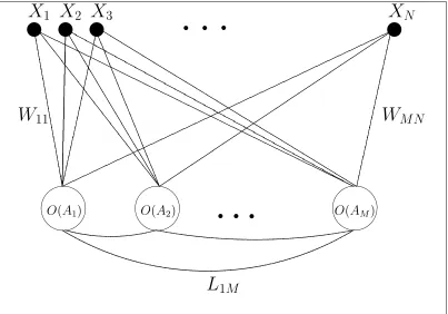
The network (fig. 3.1) which was used here has a similar architecture to the REC model proposed by Harpur and Prager [35]. It consists of M units, each of which has N inputs, the receptive fields (RFs) for different units are fully overlapping. The weight vector (of dimensionality N) for unit i is denoted by W~i,|W~i| = 1.
Unlike the original network interpretation of the REC model, this network has lateral connections Lij = −W~iW~j, which are a consequence of the error function that is
| | | s s s |
s s s &% '$ &% '$ &% '$ E E E E E E E E E E E E E E E E E E E E E E E E E E E E E E E E \ \ \ \ \ \ \ \ \ \ \ \ \ \ \ \ \ \ \ \ \ \ \ \ \ \ \ \ \ \ T T T T T T T T T T T T T T T T T T T T T T T T T T T T T T L L L L L L L L L L L L L L L L L L L L L L L L L L L L L L H H H H H H H H H H H H H H H H H H H H H H H H H H H H H H H H H H H H H H H H H H H H H H H H H H H H H H H H H H H H H H H H H H H H H H H H H H H H H H H H H H H H H H H H H H H H H H H H H H H H H H H H H H H H H H H H H H H H b b b b b b b b b b b b b b b b b b b b b b b b b b b b b b b b b b b b b b b b b b b b b b b b
X
1X
2X
3W
11W
M NO(A1) O(A2)
L
1MO(AM)
[image:40.595.105.508.51.333.2]X
NFigure 3.1: A network interpretation of the REC model. X1, . . . , XN are the
input terminals. Each unit computes the output from its activation Ai via the
transfer function O(A). The symmetric and bidirectional lateral connections are given by Lij =−W~iW~j.
a unit is given by
Oi = O(Ai) (3.1)
Ai = X ~~Wi+ M
X
j=1,j6=i
LijOj (3.2)
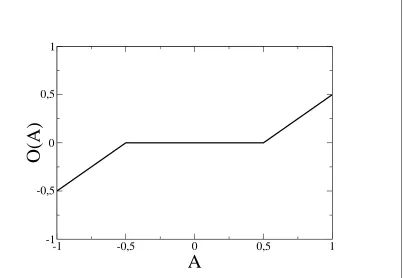
where Ai is the activation of unit i and O(A) (see fig. 3.2) is a piecewise linear
activation function with a dead-zone of width λi around 0, i.e.
−λi ≤Ai ≤λi : Oi = 0
|Ai|> λi : Oi =Ai−λisign (Ai) (3.3)
Here and in the following the sign () function is defined as
x >0 : sign (x) = 1 (3.4)
-1 -0,5 0 0,5 1
A
-1 -0,5 0 0,5 1
[image:41.595.105.508.55.333.2]O(A)
Figure 3.2: The units’ activation function for λi = 0.5
When an input vector is presented to the network, its outputs need to be determined such that the equations (3.1) and (3.2) are fulfilled simultaneously for all units.
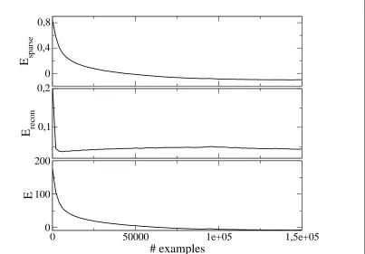
Harpur and Prager define an error function to measure reconstruction accuracy and sparseness. The error function that governs the dynamics of this network is similar, but a different λi was used for each unit which is determined by learning:
E = 1
2 X~ −
M
X
j=1
~ WjOj
!2
| {z }
Erecon
+
M
X
j=1
λj|Oj|
| {z }
Esparse
(3.5)
Erecon measures the reconstruction accuracy, andEsparseis the sparseness penalty. If
(3.1) and (3.2) are fulfilled for all units, then this error function assumes a minimum. This can readily be seen by evaluating the derivate of E with respect to Oi (for a
detailed proof, see appendix A):
∂E ∂Oi
=−X ~~Wi+ M
X
j=1
~
WiW~jOj+λisign (Oi) (3.6)
IfOi 6= 0 at the minimum, then, by substituting (3.3) and (3.2) into (3.6) (noting
that in this case sign (Oi) = sign (Ai)), one finds that (3.6) vanishes, which is a
Here, it is a sufficient condition as well as 3.5 is always positive. Should the output (at the minimum) be zero, however, then the minimum is located at a point where (3.6) is not continuous. In this case it is sufficient to require that
lim
Oi→0+
∂E ∂Oi
> 0 and
lim
Oi→0−
∂E ∂Oi
< 0 (3.7)
which is fulfilled because ∂E ∂Oi
Oi=0
=|Ai|< λi. It is this discontinuity which gives
rise to the dead-zone of the activation function: Whenever the activation of a unit is in the interval [−λi, λi], the minimum of the error function is located at Oi = 0.
The error function (3.5) is similar to that which governs the dynamics of a Hopfield network [36, 37] and it can indeed be proven that when (3.1) and (3.2) are used for asynchronous sequential (one unit at a time) updating of the network’s outputs, that the minimum of E forms a stable attractor. The proof is similar to that for an Hopfield network (see appendix B).
As theλi control the interval of activation in which the units are inactive, a unit
will not respond to any input should its λi become very large. It is then possible
to prune this unit without altering the code, since the code symbol it represents is then never used.
3.2.1
Activation algorithms
Three different activation algorithms were compared with respect to their speed, accuracy and sparseness of the resulting code. The employed sparseness measure is given by the number of inactive units (i.e. units with zero output). This is a suitable definition if the network is to be used for image coding and compression, as the outputs of inactive units need not to be stored.
3.2.2
Gradient descent with clipping
The first algorithm that was tried was an extension of simple gradient descent. Consider the case where Oi = 0 for some i at the minimum. As the sparsifier (i.e.
the sparseness-promoting penalty term λi|Oi|) is not differentiable at this point,
![Figure 3.5: Average output E [|Oi|] per example for all units of the 4x over-](https://thumb-us.123doks.com/thumbv2/123dok_us/8568164.367672/53.595.103.507.164.441/figure-average-output-e-oi-example-units-x.webp)