Baseline fusion for image an pattern recognition what not to do (and how to do better)

(1)

Journal of

Imaging

Article

Baseline Fusion for Image and Pattern

Recognition—What Not to Do (and How to Do Better)

Ognjen Arandjelovi´c

School of Computer Science, University of St Andrews, St Andrews, Fife KY16 9SX, Scotland, UK; [email protected]; Tel.: +44-(0)1334-482624

Received: 18 July 2017; Accepted: 2 October 2017; Published: 11 October 2017

Abstract: The ever-increasing demand for a reliable inference capable of handling unpredictable

challenges of practical application in the real world has made research on information fusion of major importance; indeed, this challenge is pervasive in a whole range of image understanding tasks. In the development of the most common type—score-level fusion algorithms—it is virtually universally desirable to have as a reference starting point a simple and universally sound baseline benchmark which newly developed approaches can be compared to. One of the most pervasively used methods is that of weighted linear fusion. It has cemented itself as the default off-the-shelf baseline owing to its simplicity of implementation, interpretability, and surprisingly competitive performance across a widest range of application domains and information source types. In this paper I argue that despite this track record, weighted linear fusion is not a good baseline on the grounds that there is an equally simple and interpretable alternative—namely quadratic mean-based fusion—which is theoretically more principled and which is more successful in practice. I argue the former from first principles and demonstrate the latter using a series of experiments on a diverse set of fusion problems: classification using synthetically generated data, computer vision-based object recognition, arrhythmia detection, and fatality prediction in motor vehicle accidents. On all of the aforementioned problems and in all instances, the proposed fusion approach exhibits superior performance over linear fusion, often increasing class separation by several orders of magnitude.

Keywords:prediction; arrhythmia; image matching; object recognition

1. Introduction

Score-level fusion of information is pervasive in a wide variety of problems. From predictions of the price of French vintage wine using the fusion of predictions based on rainfall and temperature data [1], to sophisticated biometrics algorithms which fuse similarity measures based on visual, infrared face appearance, or gait characteristics [2–5], the premise of information fusion is the same: the use of multiple information sources facilitates the making of better decisions [6,7].

Whatever the specific problem, the effectiveness of a specific information fusion methodology needs to be demonstrated. If possible this should be done by comparing its performance against the current state-of-the-art. However this is often prohibitively difficult in practice. For example, in some cases the state-of-the-art may not be readily available for evaluation—the original code may not have been released and re-implementation may be overly time-consuming, the algorithm may not have been described in sufficient detail, the technology may be proprietary and costly to purchase, etc. In other cases there may not be a clear state-of-the-art because the particular problem at hand has not been addressed before. In such circumstances it is useful to compare the novel methodology with a simple yet sensible baseline [8].

Probably the simplest choices for the baseline would be the performances achieved using individual information sources which are being fused. However this is an excessively low bar

(2)

for comparison. Instead what is widely done by authors across the research spectrum is to use simple weighted fusion of individual scores as a reference. In the present paper I analyse this choice, present theoretical arguments against it, and its lieu propose an alternative. The proposed alternative is inherently more principled than the aforementioned baseline, while being no more complex, either computationally or conceptually.

2. Uninformed Information Fusion

Let us start by formalizing the problem considered in this paper. I adopt the broad paradigm of so-called data source identification and matching. In particular, I assume that the available data comprises a set ofnsensed observations, X = {xi} = {x1, . . . ,xn}, which correspond to different modalities sensing the same data source. Furthermore, I assume that there are functions (i.e., algorithms)φ1, . . . ,φnwhich quantify how well a particular observationxi matches a specific data source. Without loss of generality I assume 0≤φi(xi)<∞, where 0 indicates the best possible match, and→∞the worst i.e.,φi(xi)can be thought of a quasi-distance—‘quasi-’ to emphasise that it is not required thatφi(xi)meets the strict conditions required of a metric. Note that the aforestated setting describes observations in the most general sense, e.g., these may be feature vectors (such as rasterized appearance images or SIFT descriptors in computer vision), sets of vectors, and so on, and they do not need to be of the same type (for example, some may be vectors, others sequences) or dimensionalities.

As noted in the previous section, we are looking for a simple way of fusing different matching decisionsφi(xi)in a simple manner which is a reasonable baseline in an uninformed setting, that is, without exploiting any particular properties of different functionsφ_ior observationsxi. A common one pervasively used in the literature is weighted linear fusion, which can be expressed as follows:

Φ(x1, . . . ,xn;φ1, . . . ,φn,w1, . . . ,wn) = n

∑

i=1

[wi×φi(xi)], (1)

where:

∀i=1, . . . ,n.wi≥0, and n

∑

i=1

wi =1. (2)

Here Φ(x1, . . . ,xn;φ1, . . . ,φn,w1, . . . ,wn) is the fused matching score which is derived by simply combining different φi(xi), and (2) ensures that the condition 0≤φi(xi)<∞ is maintained for Φ(x1, . . . ,xn;φ1, . . . ,φn,w1, . . . ,wn) as well, i.e., that it is the case that 0≤Φ(x1, . . . ,xn;φ1, . . . ,φn,w1, . . . ,wn)<∞.

The fusion approach described by (1) can also be rewritten more simply as:

Φ(x1, . . . ,xn;φ1, . . . ,φn,w1, . . . ,wn) = (3)

ˆ

Φ(x1, . . . ,xn;φ1, . . . ,φn,w1, . . . ,wn) = n

∑

i=1

₁

n ×φˆi(xi,wi,n)

, (4)

where:

ˆ

φi(xi,wi,n) =n×wi×φi(xi). (5)

Here the original weighted linear fusion of the contributing termsφi(xi)in (1) has been replaced by unweighted linear fusion of terms ˆφi(xi,wi,n)which adjust the magnitudes of the fused scores directly. This can be achieved simply by considering the statistics of the distributions of differentφi(xi) and the corresponding prediction, and without any knowledge of what different featuresxirepresent or what form differentφihave, i.e., while maintaining the premise of uninformed fusion.

(3)

J. Imaging2017,3, 44 3 of 16

a wide span of different data types and domains, ranging from dementia screening [9] to multimodal biometric identification [2,10].

Φo(x1, . . . ,xn;φ1, . . . ,φn,ω1, . . . ,ωn) = s _n

∑

i=1

[ωi×φi(xi)2], (6)

where as before:

∀i=1, . . . ,n.ωi≥0, and n

∑

i=1

ωi =1. (7)

Φo(x1, . . . ,xn;φ1, . . . ,φn,ω1, . . . ,ωn) = (8)

ˆ

Φo(x1, . . . ,xn;φ1, . . . ,φn,ω1, . . . ,ωn) = s _n

∑

i=1

1

n ×φei(xi,ωi,n)2

, (9)

where, analogously to (5), the adjusted fusion scores can be expressed as:

e

φi(xi,ωi,n) = √

n×ωi×φi(xi). (10)

The formulation in (9) can be readily recognized as the quadratic mean, in engineering also commonly referred to as the root mean square (RMS), of thentermsφei(xi,ωi,n).

Before proceeding with a formal analysis of the two fusion approaches, it is insightful to gain an intuitive understanding of the difference between them. Note that simple linear fusion described in (4) treats different scores as effectively interchangeable—a decrease in one score is exactly compensated by an increase in another score by the same amount. This is sensible when the scores correspond to the same measurement which is merely repeated. The described fusion can then be seen as a way of reducing measurement error, assuming that measurement is unbiased and that errors are identically and independently distributed [11]. However this is a rather trivial case of fusion and in practice one is more commonly interested in fusion of different types of data modalities. Indeed, in practice it is often the explicit aim to try to use information sources which vary independently, and attempt to exploit best their complementary natures [12]. In such instances different scores are best treated as describing a source in orthogonal directions, thereby giving rise to a feature vector

e

φ1(x1), . . . ,φen(xn) T

∈ _Rn. The quadratic mean-based fusion of (9) can then be thought of as emerging from a normalized distance measure between such feature vectors in the corresponding ambient embedding spaceRn.

Let us now consider the effects of the two fusion approaches in more detail. Firstly, note that scoring measures ˆφi(xi,wi,n) and φei(xi,ωi,n) are inevitably imperfect—neither can be expected

to produce universally the perfect matching score of 0 when the query correctly matches a source and

∞when it does not. Even the weaker requirement of universally smaller pseudo-distances for correct matches is unrealistic. Indeed, it is precisely this practical challenge that motivates multimodal fusion. Consequently, they are appropriately modelled as resulting from draws from random variables:

ˆ

φ_i(xi),φei(xi)∼Xi. (11)

Let us examine the effects of the two fusion approaches in detail. Specifically, for clarity consider the fusion of two sources, sayiandj, while observing that the derived results are readily applicable to the fusion of an arbitrary number of sources through the use of an inductive argument. Following (4) and (9), applying linear and quadratic mean-based fusion results in scores described respectively by random variables ˆYijandYeij, where:

ˆ

φi(xi) +φˆj(xj)

2 ∼

Xi+Xj

(4)

and:

s

e

φi(xi)2+φej(xj) 2

2 ∼

s

Xi2+Xj2

2 =Yije . (13)

The former can be further expanded as:

EhYijˆ 2i=E "

Xi+Xj 2

2# = 1

4

n

EhXi2i+EhXj2i+E XiXjo

, (14)

and the latter:

EhYe_ij2 i

=E 

 

s

Xi2+Xj2 2

2



 (15)

=1₂nEhXi2i+EhXj2io= ₄1n2EhXi2i+2EhXj2io. (16)

Writing:

µ_i≡E[X_i] andµ_j≡E_X

j (17)

σi≡E h

(Xi−µi)2 i

andσj ≡E h

(Xj−µj)2 i

(18)

and using the standard definition of Pearson’s correlation coefficientρ:

ρ= E[Xi−µi]E[Xj−µj]

σiσj , (19)

we can write:

EhYijˆ 2i−EhYe_ij2 i

=σi2+µi2+σj2+µj2−2 ρσiσj−µiµj (20)

=σi2+σj2−2ρσiσj+ (µi+µj)2 (21) ≥σi2+σj2−2σiσj+ (µi+µj)2 (22)

= (σ_i+σ_j)2+ (µ_i+µ_j)2≥0. (23)

Therefore: EhYijˆ 2i ≥ EhYijf 2i

. In other words, following the fusion of the same scores the proposed quadratic mean-based fusion results in lower fused matching scores (quasi-distances described by the random variableYijf) than those obtained by employing linear fusion (described

by the random variable ˆYij).

(5)

J. Imaging2017,3, 44 5 of 16

preferentially and systematically to produce lower scores for correctly matching sources and higher scores for incorrectly matching sources. Therefore, while non-matching comparisons may result in some of the fused scores erroneously to be low, on average such errors should exhibit a lower degree of correlation than low scores across different modalities do for correct matches. In the next section I will demonstrate that this indeed is the case in practice.

3. Experimental Section

Having laid out the theoretical argument against simple weighted combination as the default baseline for uninformed fusion, in favour of the quadratic mean, in this section the two are compared empirically. In Section3.1I begin by describing experiments on synthetic data, which allow the characteristics of the two approaches to be studied in a carefully controlled fashion, and then proceed with experiments on real, challenging data sets of vastly different types. In particular, the popular computer vision problem of image-based object recognition is used as a case study in Section3.2, arrhythmia prediction in Section3.3, and finally fatality prediction in road vehicle accidents in Section3.4.

3.1. Synthetic Data

I start my comparative analysis with a simple synthetic example involving the fusion of two information sources. The main goal of this experiment is twofold. Firstly it is to examine if empirical results obtained in controlled and well understood conditions are consistent with the theoretical prediction of superior performance of the proposed quadratic mean-based fusion in comparison with the common linear fusion-based approach. My second aim is to investigate if the differential advantage of the proposed method indeed varies in accordance to the degree to which the fused information sources are correlated.

In this experiment I adopt a generative model which comprises two modalities which are used to sense two information sources. The model thus generates a set of observations:

(

{x1,1,x1,2},{x2,1,x2,2}, . . .

)

(24)

wherexi,j is thei-th measurement using thej-th modality (wherej = 1, 2). For a given modality, i.e., for fixedj, differentxi,j are independent and identically distributed samples. A measurement xi,1is generated by a random draw from the ground truth distribution represented by the random variableG1and corrupting it by a random draw from the noise distribution represented by the random variableGn:

di,1∼G1=N(0, 1), (25)

ni,1∼Gn =N(0, 1), (26)

xi,1=di,1+βn×ni,1. (27)

On the other hand, a measurementxi,2is generated using in part a process independent of the measurementxi,1and in part dependent on it. The former contribution is generated as per (25)–(27) while the latter is modelled using a weighted contribution ofxi,1. Formally:

di,2∼G1=N(0, 1), (28)

ni,2∼Gn=N(0, 1), (29)

xi,2=ρ×xi,2+q1−ρ2×di,2+βn×ni,2 (30)

(6)

Lastly, the quasi-similarity functions φj which quantify how well an observation matches a particular information source are computed as:

ˆ

φ₁(1)(xi,1) =|xi,1|, (31)

ˆ

φ₂(1)(xi,2) =|xi,2|. (32)

ˆ

φ₁(2)(xi,1) =|∆−xi,1|, (33)

ˆ

φ₂(2)(xi,2) =|∆−xi,2|. (34)

where∆models the separation (dissimilarity) between the two information sources. Note that all ˆφ(qk)(xi,j) are already normalized to be in the range assumed in Section1, that is∀i,j,k,q. ˆφ(qk)(xi,j)∈[0,∞).

3.1.1. Results, Analysis and Discussion

I compared the performance of the two fusion approaches discussed in Section2by computing fused quasi-similarities between the generated data and the two information sources as per (31)–(34). Specifically, the linearly fused quasi-similarity of ˆφ₁(1)(x_i,1)and ˆφ₁(1)(x_i,2)was computed as:

1 2

ˆ

φ₁(1)(x_i,1) +φˆ₁(1)(x_i,2), (35)

and similarly of of ˆφ(₁2)(xi,1)and ˆφ₁(2)(xi,2)was computed as:

1 2

ˆ

φ₁(2)(x_i,1) +φˆ₁(2)(x_i,2). (36)

The proposed quadratic-mean-based fusions were computed as respectively:

s

1 2

ˆ

φ(₁1)(xi,1)2+φˆ₁(1)(xi,2)2

. (37)

and:

s

1 2

ˆ

φ(₁2)(xi,1)2+φˆ₁(2)(xi,2)2

. (38)

To evaluate and compare the two methods I examined the corresponding differential matching scores computed for the correct and incorrect information sources, that is:

∂1=φˆ(₁1)(xi,1)−φˆ1(2)(xi,1) =|xi,1| − |∆−xi,1|, (39)

for the linear fusion, and

∂2=φˆ(₂1)(xi,2)−φˆ₂(2)(xi,2) =|xi,2| − |∆−xi,2|. (40)

(7)

J. Imaging2017,3, 44 7 of 16

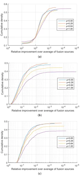
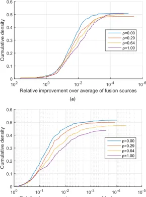
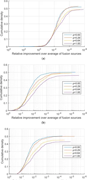
between 0.10 and 5.00), andρ ∈ {0.00, 0.29, 0.64, 1.00}(approximately linearly equidistant values between 0.00 and 1.00).

I started my analysis on the coarsest level by examining the proportion of cases in which the proposed method was at least as successful as the alternative, that is, the proportion of cases in which ∂1≤∂2. Already at this stage the findings were decisively in favour of the proposed approach which neverdid worse than linear fusion across all combinations ofβnandρ. In approximately 50% of the cases my method performed equally well as linear fusion and in the remaining 50% of the cases effected an improvement. A more detailed insight is offered by the plots in Figures1–3which show the cumulative density distribution of the relative improvement achieved by the proposed method, that is(∂2−∂1)/∂1when the source was correctly matched, across different experiments. For example from Figure1it can be seen that the matching score separation increased twofold (corresponding to the abscissa value of 100_{) in approximately 20% of the cases for the three experiments with}_β_n ₌_0.05, and in approximately 15% of the cases for the three experiments withβn=0.32 from Figure2, while in the three experiments withβn =3.00 the relative differential matching score increase of this degree was rare (Figure3). A comparison of the plots in the three figures further reveals that the dissimilarity between information sources has little effect on the average benefit of the proposed method. However the value of∆did affect performances for different values ofρ. Specifically, across Figures1–3it can be seen that for small values of∆, that is, for very similar information sources that we are seeking to discriminate between, the proposed fusion methodology offered approximately equal benefits over linear fusion for different values ofρ. In other words the redundancy of the two sensed modalities, or lack thereof, had little effect. In contrast, as the information sources become more separated (increasing∆), the greater the effect ofρbecomes, with the proposed method offering the greatest advantage when the sensed modalities are complementary i.e., whenρ=0.

3.2. Object Recognition

In a controlled experiment using synthetic data and and well-understood information sources, I demonstrated both the superior performance of the proposed generic fusion approach over the common alternative in the form of linear fusion, as well as the consistency of its behaviour with theoretical expectations put forward previously. I next set out to examine whether the same advantages are observed when real-world data is used instead. After all, recall that the central aim of the present paper is to scrutinize the soundness of linear fusion as a generic baseline and argue in favour of the described quadratic mean-based fusion as an alternative with superior performance but paralleled quasi-universality and simplicity of implementation.

My first case-study involves computer-based object recognition. This is an important problem in the spheres of computer vision and pattern recognition, and which has potential for use in a wide spectrum of practical applications. Examples range from motorway toll booths that automatically verify that the car type and its licence plate match the registration database, to online querying and searching for an object of interest that was captured using a mobile phone camera. Object recognition has attracted much research attention [13–16] and this interest has particularly intensified in recent years after significant advances towards practically viable systems have been made [15–17].

(8)

an analogous descriptor of local shape for the characterization of shape [19]. In both cases descriptors are matched using the Euclidean distance.Version September 29, 2017 submitted toJ. Imaging 12 of 23

Relative improvement over average of fusion sources 10-6 10-4 10-2 100 102 104 Cumul ative density 0.1 0.2 0.3 0.4 0.5 0.6 ρ=0.00 ρ=0.29 ρ=0.64 ρ=1.00

(a)βn=0.05,d=0.10

Relative improvement over average of fusion sources 10-5 10-4 10-3 10-2 10-1 100 Cumul ative density 0 0.1 0.2 0.3 0.4 0.5 ρ=0.00 ρ=0.29 ρ=0.64 ρ=1.00

(b)βn=0.05,d=2.28

[image:8.595.166.431.121.712.2] [image:8.595.168.427.132.294.2]

(c)βn=0.05,d=5.00

Figure 1.Synthetic data: relative improvement in the confidence of the correct information source identification of the proposed quadratic mean-based fusion over linear fusion, as the corresponding cumulative distribution function.

(a)

Version September 29, 2017 submitted toJ. Imaging 12 of 23

(a)βn=0.05,d=0.10

(b)βn=0.05,d=2.28

(c)βn=0.05,d=5.00

(b)

(a)βn=0.05,d=0.10

(b)βn=0.05,d=2.28

(c)βn=0.05,d=5.00

(c)

(9)

J. Imaging_{Version September 29, 2017 submitted to}2017,3, 44 _{J. Imaging} _{13 of 23}9 of 16

Relative improvement over average of fusion sources

10-6 10-4 10-2 100 102 Cumul ative density 0 0.1 0.2 0.3 0.4 0.5 0.6 ρ=0.00 ρ=0.29 ρ=0.64 ρ=1.00

(a)βn=0.32,d=0.10

Relative improvement over average of fusion sources 10-5 10-4 10-3 10-2 10-1 100 Cumul ative density 0 0.1 0.2 0.3 0.4 0.5 0.6 ρ=0.00 ρ=0.29 ρ=0.64 ρ=1.00

(b)βn=0.32,d=2.28

Relative improvement over average of fusion sources 10-6 10-5 10-4 10-3 10-2 10-1 100 Cumul ative density 0 0.1 0.2 0.3 0.4 0.5 ρ=0.00 ρ=0.29 ρ=0.64 ρ=1.00

[image:9.595.153.444.92.483.2] [image:9.595.154.442.93.270.2]

(c)βn=0.32,d=5.00

(a)

(a) βn=0.32,d=0.10

(b)βn=0.32,d=2.28

(c) βn=0.32,d=5.00

(b)

(a) βn=0.32,d=0.10

(b)βn=0.32,d=2.28

(c) βn=0.32,d=5.00

(c)

(10)

Relative improvement over average of fusion sources 10-6 10-4 10-2 100 102 104 Cumul ative density 0 0.1 0.2 0.3 0.4 0.5 0.6 ρ=0.00 ρ=0.29 ρ=0.64 ρ=1.00

(a) βn=3.00,d=0.10

Relative improvement over average of fusion sources 10-6 10-5 10-4 10-3 10-2 10-1 100 Cumul ative density 0 0.1 0.2 0.3 0.4 0.5 0.6 ρ=0.00 ρ=0.29 ρ=0.64 ρ=1.00

(b)βn=3.00,d=2.28

[image:10.595.152.444.92.694.2] [image:10.595.154.441.92.269.2]

(c) βn=3.00,d=5.00

(a)

10-6 10-4 10-2 100 102 104 Cumul ative density 0 0.1 0.2 0.3 0.4 0.5 0.6 ρ=0.00 ρ=0.29 ρ=0.64 ρ=1.00

(a)βn=3.00,d=0.10

(b)βn=3.00,d=2.28

(c)βn=3.00,d=5.00

(b)

10-6 10-4 10-2 100 102 104 Cumul ative density 0 0.1 0.2 0.3 0.4 0.5 0.6 ρ=0.00 ρ=0.29 ρ=0.64 ρ=1.00

(a)βn=3.00,d=0.10

(b)βn=3.00,d=2.28

(c)βn=3.00,d=5.00

(c)

(11)

J. Imaging2017,3, 44 11 of 16

As in the preceding section in which synthetic data was used, fused quasi-similarities between the observed data and the two information sources were computed as per (31)–(34), and their performance assessed by analysing the corresponding differential matching scores computed for the correct and incorrect information sources as detailed previously and summarized by (39) and (40).

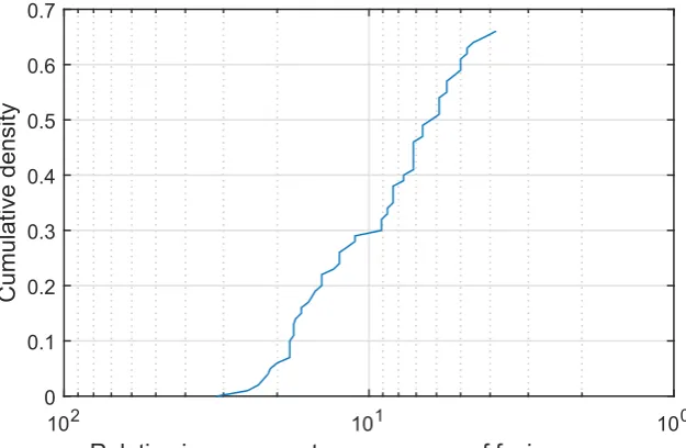
I display my findings in Figure4which shows a plot of the cumulative density distribution of the relative improvement achieved by the proposed method (as before please note that the abscissa scale is logarithmic and that it is increasing in the leftward direction). Firstly let us make the highly encouraging observation that the same qualitative behaviour of this characteristic plot is exhibited on this real-world data set as on the synthetic data of the previous experiment. Remarkably, in all cases the proposed fusion strategy did at least as well as the simple weighted fusion. In approximately 66% of the cases the proposed quadratic fusion exhibited superior performance, performing on par in the remaining 34% of the cases. A further examination of the plot reveals an even stronger case for the proposed method—not only does it outperform simple weighted fusion in 66% of the cases but it does so with a great margin. For example in 30% of the cases the inter-class separation is increased 10-fold (i.e., by an order of magnitude).

Relative improvement over average of fusion sources

100 101

102

Cumul

ative density

[image:11.595.141.454.326.530.2]

0 0.1 0.2 0.3 0.4 0.5 0.6 0.7

Figure 4.General object recognition: relative improvement in the correct information source identification of the proposed quadratic mean-based fusion over linear fusion, as the corresponding cumulative distribution function.

and informed healthcare provision to the population at risk of cardiac complications. This primarily includes

185

individuals with preexisting cardiac problems or congenital factors, which are further modulated by various

186

environmental factors such as high physical exertion [20] or the use of certain classes of drugs.

187

A normally functioning human heart maintains a remarkably well controlled heartbeat rhythm. Arrhythmias

188

are abnormalities of this rhythm and are caused by physiological factors pertaining to electrical impulse generation

189

or propagation. Arrhythmia types can be grouped under the umbrellas of three broad categories: tachycardias

190

(overly high heartbeat rate), bradycardias (overly low heartbeat rate), and arrhythmias with an irregular heartbeat

191

rate. While most arrhythmias are transient in nature and do not pose a serious health risk, some arrhythmias

192

(particularly in high risk populations) can have serious consequences such as stroke, cardiac arrest, or heart

193

failure and death [21].

194

Arrhythmias can be diagnosed using nonspecific means, e.g. using a stethoscope or a tactile detection

195

of pulse, or specific methods and in particular the electrocardiogram (ECG). Moreover, the rich information

196

provided by the latter can be used to predict and detect the onset of arrhythmias by analysing electric impulse

197

patterns [22]. In the present study I evaluate the proposed fusion methodology in the context of this prediction.

198

Figure 4. General object recognition: relative improvement in the correct information source identification of the proposed quadratic mean-based fusion over linear fusion, as the corresponding cumulative distribution function.

3.3. Arrhythmia Prediction

My second real-world case-study concerns automatic arrhythmia prediction from demographic data and physiological measurements. This is a challenging task of enormous importance in the provision of timely and informed healthcare provision to the population at risk of cardiac complications. This primarily includes individuals with preexisting cardiac problems or congenital factors, which are further modulated by various environmental factors such as high physical exertion [20] or the use of certain classes of drugs.

(12)

and do not pose a serious health risk, some arrhythmias (particularly in high risk populations) can have serious consequences such as stroke, cardiac arrest, or heart failure and death [21].

Arrhythmias can be diagnosed using nonspecific means, e.g., using a stethoscope or a tactile detection of pulse, or specific methods and in particular the electrocardiogram (ECG). Moreover, the rich information provided by the latter can be used to predict and detect the onset of arrhythmias by analysing electric impulse patterns [22]. In the present study I evaluate the proposed fusion methodology in the context of this prediction.

[image:12.595.127.467.378.465.2]

I used the dataset collected by Guvenir et al. [22] which is freely available online and can be downloaded [23]. The dataset comprises a rich set of demographic and antropometric variables, such as each person’s age, sex, height, and bodyweight, as well as a variety of features extracted from the person’s ECG, including the heart rate and a series of characteristics of the corresponding signal deflections (the duration of the QRS interval, amplitudes of Q, R, and S waves etc.); please refer to the original publication for full detail [22]. The target variable for the purpose of the present experiment can be considered to be binary valued, taking on the value 0 when arrhythmia is not present and 1 when it is; please see Table1.

Table 1.An illustration of the adopted arrhythmia dataset, originally collected and described in detail by Guvenir et al. [22]. It comprises 279 input variables, of which only a small selection is shown here, and the corresponding target variable which for the purpose of the present experiment can be considered to be binary valued, taking on the value 0 when arrhythmia is not diagnosed and 1 when it is.

Age Gender Height Body Weight QRS Duration

. . . Arrythmia

(Years) (cm) (kg) (ms) (Yes/No)

75 Male 190 80 91 . . . Yes

56 Female 165 64 81 . . . Yes

. . . .

55 Male 175 94 100 . . . No

. . . .

I consider two baseline classifiers. The first of these takes height, bodyweight, and the duration of the QRS interval as input variables (i.e., independent variables). The second one makes the prediction based on what are effectively integrals of Q, R, and S deflections (i.e., referred to as QRSA in the dataset description; please see the original reference for detail [22]), and the Q, R, S, and T deflections (i.e., referred to as QRSTA in the dataset description. Each classifier is built upon a generalized linear model (GLM) [24]. Recall that in a GLM the meanE[Y]of the target, outcome variableYis related to a linear predictor based on the independent variables through a link functionL:

E[Y]≡µ=L−1(1+αx). (41)

The variance Var[Y]ofYis modelled as a functionVof this mean:

Var[Y] =V(µ) =V(L−1(1+αx)). (42)

In my experiment, the continuous output of a GLM is used to detect the presence of arrhythmia using what is effectively the nearest neighbour criterion: if the output is closer to 0 the prediction is taken to be negative, and if it is closer to 1 positive. The dataset contains 452 diagnosis cases of which 100 were used for training the classifiers; the remaining 352 were used for testing.

(13)

J. Imaging2017,3, 44 13 of 16

corresponding differential matching scores computed for the correct and incorrect information sources as detailed previously and summarized by (39) and (40).

I display my findings in Figure5, which shows a plot of the cumulative density distribution of the relative improvement achieved by the proposed method (as before please note that the abscissa scale is logarithmic and that it is increasing in the leftward direction). We can again start with the observation which can be made by comparing the characteristics of the plot in Figure5with those of the plots in Figure4and Figures1–3and observing that again the same qualitative behaviour is exhibited on this data too. In all cases the proposed fusion strategy did at least as well as the simple weighted fusion, with approximately 65% of the cases resulting in superior performance of the proposed quadratic fusion and the remaining 35% in on a par performance. As in the previous experiments when my method outperforms simple weighted fusion it does so with a significant margin with an over doubled separation increase in approximately 16% of the cases. Moreover I found that while simple weighted fusion failed to improve the prediction of the better performing baseline classifier in 15% of the cases, the same was the case with the proposed method in fewer than 7.8% of the cases.

10-2 10-1

100 101

Cumul

ative density

[image:13.595.142.452.302.498.2]

0 0.1 0.2 0.3 0.4 0.5 0.6 0.7

Figure 5.Arrhythmia prediction: relative improvement in the correct information source identification of the proposed quadratic mean-based fusion over linear fusion, as the corresponding cumulative distribution function.

through the Fatality Analysis Reporting System (FARS) for the year 2011. These are freely publicly available2_.

230

The dataset comprises a number of person specific variables, such as age, sex, race, blood alcohol level, and

231

drug use status, as well as a variety of variables pertaining to the context of the accident, including the type

232

of the road and the state where the accident took place, and the weather conditions at the time (please see

233

http://www-fars.nhtsa.dot.gov/Main/index.aspxfor full description). The target variable for the purpose of the

234

present experiment can be considered to be binary valued, taking on the value 1 when there has been a fatality

235

and 0 otherwise; please see Table2.

236

As in the previous experiment I consider two baseline classifiers, each built upon a generalized linear model.

237

The first of these takes the person’s age and blood alcohol level as input variables (i.e. independent variables).

238

The second one makes the prediction based on atmospheric conditions and the road type. Following the same

239

framework as described in the previous section, the continuous output of a GLM is used to predict the occurrence

240

of a fatality using what is effectively the nearest neighbour criterion: if the output is closer to 0 the prediction is

241

taken to be negative, and if it is closer to 1 positive. The dataset contains 5000 accidents of which 1000 randomly

242

2 _{The dataset can be downloaded from}_{http://www-fars.nhtsa.dot.gov/Main/index.aspx}_.

Figure 5.Arrhythmia prediction: relative improvement in the correct information source identification of the proposed quadratic mean-based fusion over linear fusion, as the corresponding cumulative distribution function.

3.4. Car Accident Fatality Prediction

(14)

[image:14.595.143.453.162.249.2]

Table 2.An illustration of the adopted car accidents dataset released by the government of the USA through the Fatality Analysis Reporting System (FARS) for the year 2011. It comprises 15 input variables, of which only a selection is shown here, and the corresponding target variable which for the purpose of the present experiment can be considered to be binary valued, taking on the value 1 when there has been a fatality and 0 when not.

Clear Atmospheric Driver Alcohol Driver

. . . Fatalities

Conditions (Yes/No) Age Blood Level Gender (Yes/No)

Yes 27 0 Male . . . No

Yes 60 0 Female . . . Yes

. . . .

No 20 0.21 Male Yes

. . . .

As in the previous experiment, I consider two baseline classifiers, each built upon a generalized linear model. The first of these takes the person’s age and blood alcohol level as input variables (i.e., independent variables). The second one makes the prediction based on atmospheric conditions and the road type. Following the same framework as described in the previous section, the continuous output of a GLM is used to predict the occurrence of a fatality using what is effectively the nearest neighbour criterion: if the output is closer to 0 the prediction is taken to be negative, and if it is closer to 1 positive. The dataset contains 5000 accidents of which 1000 randomly selected cases were used for training the baseline classifiers with the remainder employed for performance evaluation.

(15)

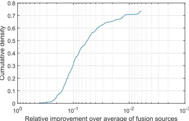
J. Imaging2017,3, 44 15 of 16 Version September 29, 2017 submitted toJ. Imaging 21 of 23

rather than of some algorithmic aspect of the proposed method. In other words, the lesser advantage (though still

261

consistent and observed in an overwhelming number of cases) of using the proposed method stems from greater

262

redundancy across the fused information sources.

263

Relative improvement over average of fusion sources

10-3 10-2

10-1 100

Cumul

ative density

[image:15.595.141.453.90.290.2]

0 0.1 0.2 0.3 0.4 0.5 0.6 0.7 0.8

Figure 6.Car accident fatality prediction: relative improvement in the correct information source identification of the proposed quadratic mean-based fusion over linear fusion, as the corresponding cumulative distribution function.

4. Summary and conclusions 264

This paper considered the task of designing a score-level fusion methodology which is simple, clear, and

265

generic in its approach, allowing it to be used widely as a reasonable baseline against which novel fusion

266

approaches can be compared. In most cases the existing literature adopts simple weighted linear fusion to this end.

267

I argued that this is not a good choice in that an equally simple but more effective alternative can be formulated

268

in the shape of quadratic mean-based fusion. The argument was founded on theoretical grounds and was further

269

supported using an intuitive interpretation of the derived theoretical results, and lastly demonstrated using a

270

comprehensive series of experiments on a diverse set of fusion problems. The superiority of the proposed fusion

271

approach was first demonstrated using a classification test on synthetically generated data, and then followed by

272

three problems of major research interest: computer vision-based object recognition, ECG-based arrhythmia

273

detection, and fatality prediction in motor vehicle accidents.

274

Figure 6. Car accident fatality prediction: relative improvement in the correct information source identification of the proposed quadratic mean-based fusion over linear fusion, as the corresponding cumulative distribution function.

4. Summary and Conclusions

This paper considered the task of designing a score-level fusion methodology which is simple, clear, and generic in its approach, allowing it to be used widely as a reasonable baseline against which novel fusion approaches can be compared. In most cases the existing literature adopts simple weighted linear fusion to this end. I argued that this is not a good choice in that an equally simple but more effective alternative can be formulated in the shape of quadratic mean-based fusion. The argument was founded on theoretical grounds and was further supported using an intuitive interpretation of the derived theoretical results, and lastly demonstrated using a comprehensive series of experiments on a diverse set of fusion problems. The superiority of the proposed fusion approach was first demonstrated using a classification test on synthetically generated data, and then followed by three problems of major research interest: computer vision-based object recognition, ECG-based arrhythmia detection, and fatality prediction in motor vehicle accidents.

Conflicts of Interest:The author declares no conflict of interest.

References

1. Ginsburgh, V.; Monzak, M.; Monzak, A. Red wines of Médoc: What is wine tasting worth? J. Wine Econ. 2013,8, 159–188.

2. Guan, Y.; Wei, X.; Li, C.T.; Keller, Y.People Identification and Tracking through Fusion of Facial and Gait Features; Springer International Publishing: Cham, Switzerland, 2014; pp. 209–221.

3. Ghiass, R.S.; Arandjelovi´c, O.; Bendada, A.; Maldague, X. Infrared face recognition: A literature review. In Proceedings of the IEEE International Joint Conference on Neural Networks, Dallas, TX, USA, 4–9 August 2013; pp. 2791–2800.

4. Martin, R.; Arandjelovi´c, O. Multiple-object tracking in cluttered and crowded public spaces. Proc. Int. Symp. Vis. Comput.2010,3, 89–98.

5. Arandjelovi´c, O. Colour invariants under a non-linear photometric camera model and their application to face recognition from video. Pattern Recognit.2012,45, 2499–2509.

(16)

7. Arandjelovi´c, O.; Hammoud, R.I.; Cipolla, R. Multi-sensory face biometric fusion (for personal identification). In Proceedings of the IEEE International Workshop on Object Tracking and Classification Beyond the Visible Spectrum, New York, NY, USA, 17–22 June 2006; pp. 128–135.

8. Arandjelovi´c, O. Learnt quasi-transitive similarity for retrieval from large collections of faces. In Proceedings of the IEEE Conference on Computer Vision and Pattern Recognition, Las Vegas, NV, USA, 27–30 June 2016; pp. 4883–4892.

9. Mackinnon, A.; Mulligan, R. Combining cognitive testing and informant report to increase accuracy

in screening for dementia. Am. J. Psychiatry1998,155, 1529–1535.

10. Arandjelovi´c, O.; Hammoud, R.I.; Cipolla, R. Thermal and reflectance based personal identification methodology in challenging variable illuminations. Pattern Recognit.2010,43, 1801–1813.

11. Bishop, C.M.Pattern Recognition and Machine Learning; Springer: New York, NY, USA, 2007.

12. Arandjelovi´c, O.; Cipolla, R. A new look at filtering techniques for illumination invariance in automatic face recognition. In Proceedings of the IEEE 7th International Conference on Automatic Face and Gesture Recognition, Southampton, UK, 10–12 April 2006; pp. 449–454.

13. Aggarwal, G.; Roth, D. Learning a Sparse Representation for Object Detection. In Proceedings of the European Conference on Computer Vision, Copenhagen, Denmark, 29 April 2002.

14. Ahmadyfard, A.; Kittler, J. A comparative study of two object recognition methods. In Proceedings of the British Machine Vision Conference, Cardiff, UK, 2–5 September 2002; pp. 1–10.

15. Arandjelovi´c, R.; Zisserman, A. Smooth Object Retrieval using a Bag of Boundaries. In Proceedings of the IEEE International Conference on Computer Vision, Barcelona, Spain, 6–13 November 2011; pp. 375–382. 16. Belhumeur, P.N.; Kriegman, D.J. What is the Set of Images of an Object Under All Possible Illumination

Conditions? Int. J. Comput. Vis.1998,28, 245–260.

17. Sivic, J.; Russell, B.; Efros, A.; Zisserman, A.; Freeman, W. Discovering object categories in image collections. In Proceedings of the IEEE International Conference on Computer Vision, Beijing, China, 15–21 October 2005; pp. 370–377.

18. Arandjelovi´c, O. Matching Objects across the Textured–Smooth Continuum. In Proceedings of the Australasian Conference on Robotics and Automation, Wellington, New Zealand, 3–5 December 2012; pp. 354–361.

19. Arandjelovi´c, O. Object matching using boundary descriptors. In Proceedings of the British Machine Vision Conference, Surrey, UK, 3–7 September 2012.

20. Lengyel, C.; Orosz, A.; Hegyi, P.; Komka, Z.; Udvardy, A.; Bosnyák, E.; Trájer, E.; Pavlik, G.; Tóth, M.; Wittmann, T.; Papp, J.G.; Varró, A.; Baczkó, I. Increased Short-Term Variability of the QT Interval in Professional Soccer Players: Possible Implications for Arrhythmia Prediction. PLoS ONE2011,6, e18751. 21. Myerburg, R.J.; Interian, A.J.; Mitrani, R.M.; Kessler, K.M.; Castellanos, A. Frequency of Sudden Cardiac

Death and Profiles of Risk. Am. J. Cardiol.1997,80(Suppl. 2), 10F–19F.

22. Guvenir, H.A.; Acar, B.; Demiroz, G.; Cekin, A. A Supervised Machine Learning Algorithm for Arrhythmia Analysis. In Proceedings of the Computers in Cardiology Conference, Lund, Sweden, 7–10 September 1997; pp. 433–436.

23. Guvenir, H.A. UCI. Available online: http://archive.ics.uci.edu/ml/datasets/Arrhythmia(accessed on 11 October 2017).

24. Nelder, J.; Wedderburn, R. Generalized Linear Models.Proc. R. Soc. Ser. A1972,135, 370–384.

25. NHTSA. Available online:http://www-fars.nhtsa.dot.gov/Main/index.aspx(accessed on 11 October 2017).

c