warwick.ac.uk/lib-publications
Manuscript version: Author’s Accepted Manuscript
The version presented in WRAP is the author’s accepted manuscript and may differ from the
published version or Version of Record.
Persistent WRAP URL:
http://wrap.warwick.ac.uk/106568
How to cite:
Please refer to published version for the most recent bibliographic citation information.
If a published version is known of, the repository item page linked to above, will contain
details on accessing it.
Copyright and reuse:
The Warwick Research Archive Portal (WRAP) makes this work by researchers of the
University of Warwick available open access under the following conditions.
Copyright © and all moral rights to the version of the paper presented here belong to the
individual author(s) and/or other copyright owners. To the extent reasonable and
practicable the material made available in WRAP has been checked for eligibility before
being made available.
Copies of full items can be used for personal research or study, educational, or not-for-profit
purposes without prior permission or charge. Provided that the authors, title and full
bibliographic details are credited, a hyperlink and/or URL is given for the original metadata
page and the content is not changed in any way.
Publisher’s statement:
Please refer to the repository item page, publisher’s statement section, for further
information.
Simultaneous Localization and Mapping with Power
Network Electromagnetic Field
Chris Xiaoxuan Lu
University of Oxford
[email protected]
Yang Li
∗Shenzhen University
[email protected]
Peijun Zhao
University of Oxford
[email protected]
Changhao Chen
University of Oxford
[email protected]
Linhai Xie
University of Oxford
[email protected]
Rui Tan
Nanyang Technological
University
[email protected]
Hongkai Wen
University of Warwick
hongkai.wen@dcs.
warwick.ac.uk
Niki Trigoni
University of Oxford
[email protected]
ABSTRACT
Various sensing modalities have been exploited for indoor location sensing, each of which has well understood limita-tions, however. This paper presents a first systematic study on using the electromagnetic field (EMF) induced by a build-ing’s electric power network for simultaneous localization and mapping (SLAM). A basis of this work is a measurement study showing that the power network EMF sensed by either a customized sensor or smartphone’s microphone as a side-channel sensor is spatially distinct and temporally stable. Based on this, we design a SLAM approach that can reliably detect loop closures based on EMF sensing results. With the EMF feature map constructed by SLAM, we also design an efficient online localization scheme for resource-constrained mobiles. Evaluation in three indoor spaces shows that the power network EMF is a promising modality for location sensing on mobile devices, which is able to run in real time and achieve sub-meter accuracy.
CCS CONCEPTS
•Human-centered computing→ Ubiquitous and mobile computing;
∗This work was completed while Yang Li was with Advanced Digital
Sci-ences Center, Illinois at Singapore.
Permission to make digital or hard copies of all or part of this work for personal or classroom use is granted without fee provided that copies are not made or distributed for profit or commercial advantage and that copies bear this notice and the full citation on the first page. Copyrights for components of this work owned by others than ACM must be honored. Abstracting with credit is permitted. To copy otherwise, or republish, to post on servers or to redistribute to lists, requires prior specific permission and/or a fee. Request permissions from [email protected].
MobiCom ’18, October 29-November 2, 2018, New Delhi, India
© 2018 Association for Computing Machinery. ACM ISBN 978-1-4503-5903-0/18/10. . . $15.00 https://doi.org/10.1145/3241539.3241540
KEYWORDS
Electromagnetic field sensing; Power line network; Simulta-neous localization and mapping; Indoor localization
ACM Reference Format:
Chris Xiaoxuan Lu, Yang Li, Peijun Zhao, Changhao Chen, Linhai Xie, Rui Tan, Hongkai Wen, and Niki Trigoni. 2018. Simultane-ous Localization and Mapping with Power Network Electromag-netic Field. InThe 24th Annual International Conference on Mobile Computing and Networking (MobiCom ’18), October 29-November
2, 2018, New Delhi, India.ACM, New York, NY, USA, 16 pages.
https://doi.org/10.1145/3241539.3241540
1
INTRODUCTION
Recent years have seen the increasing need of location aware-ness by mobile applications. As of November 2017, 62% of the top 100 free Android Apps on Google Play require location services. While GPS can provide outdoor locations with sat-isfactory accuracy, indoor location sensing for mobiles has been a hard problem. Research in the last two decades has exploited various sensing modalities for indoor location sens-ing. Examples include various radio frequency (RF) signals (e.g., WiFi [11, 16, 50, 51], GSM [17], FM radio [6]), visible light [49, 52, 55], imaging [10, 13, 14, 54], acoustics [41], and geomagnetism [12, 18, 22, 35, 36, 44]. However, each sensing modality bears some limitations. RF signals have change-able propagation paths and received signal strengths (RSSes) due to barriers and transmitters’ dynamic power control. Visual lights are vulnerable to blockage. Imaging is power demanding and privacy breaching. Geomagnetic sensing is susceptible to change of altitude.
radiations (EMRs) from the powerlines in a building will form an ambient EMF. The noises induced by the power network EMF at electronic devices, calledmains hums, are undesirable in general and often removed by the devices’ built-in filters. However, recent studies leveraged the peri-odic and synchronous properties of the mains hums to design clock synchronization approaches for indoor sensors [33] and wearables [48]. Moreover, a study in [23] shows that the mains hums sensed by indoor mote-class sensors carry time information with sub-second resolution, due to the subtle but spatially homogeneous imperfections in the mains hum’s pe-riodicity. While the powerline EMR’s time-related properties have been the focus of existing studies, the spatial properties of power network EMF and whether these properties can be exploited for indoor location sensing have received no systematic research.
Hypothetically, as the powerline EMR intensity decays with the physical distance from the emitting powerline, the power network EMF formed by the superposition of the EMRs from the permanent powerlines running in the build-ing infrastructures will give a spatially distinct but tempo-rally stable intensity field, which is a basis for location sens-ing. To verify our intuition, we use two types of sensors, i.e., a customized EMR receiver and smartphone microphone, to conduct extensive measurements in various buildings. The EMR receiver is based on a tank circuit tuned to the power network’s nominal frequency, while the smartphone micro-phone can perform side-channel sensing due to the leaked mains hum in audio recordings. Our measurement results confirm positively our hypothesis in the domain of indoor pedestrian walkways. In particular, compared with geomag-netic fields that often show altitude-varying intensity, power network EMFs exhibit better altitude-invariability, suggest-ing that the power network EMF-based location senssuggest-ing can be less susceptible to user height.
Based on the measurement study, we design a Simulta-neous Localization and Mapping (SLAM) approach exploit-ing the unique characteristics of power network EMF. Our approach jointly estimates both the user locations and the power network EMF feature map of the workspace, without labor-intensive surveying or fingerprinting. The constructed power network EMF feature map is metrically consistent, where locations are associated with corresponding power network EMF signatures. In particular, we bespoke our SLAM approach for the power network EMF modality, and design novel loop closure detection and curation algorithms to reli-ably recognize previously visited locations from the observed power network EMF signals. This is of crucial importance for SLAM using power network EMF, as standard techniques (e.g. directly comparing the EMF signals at different locations) would produce many false positive loop closure proposals,
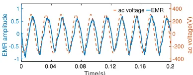
0 0.04 0.08 0.12 0.16 0.2
Time(s)
-1 -0.5 0 0.5 1
EMR amplitude
EMR
0 0.04 0.08 0.12 0.16 0.2
-400 -200 0 200 400
ac voltage(V)
[image:3.612.340.534.80.156.2]ac voltage
Figure 1: The normalized EMR amplitude around a live wire and the ac voltage between the live wire and the neutral wire.
and thus significantly jeopardize the consistency of the fea-ture map and deteriorate localization performance. Given the constructed power network EMF feature map, we also design an efficient online localization scheme capable of positioning the user in real time on resource-constrained devices.
We evaluate the proposed SLAM approach in realistic indoor/semi-outdoor environments including a lab space, an office building and a shopping center. The evaluation shows that, (i) with the customized EMR sensor, we can construct the power network EMF feature maps with sub-meter accu-racy, and achieve meter level localization with the registered maps, (ii) on commercially off-the-shelf (COTS) platforms, the composite modality of geomagnetism and power net-work EMF (sensed through microphone) can have compara-ble performance, and (iii) by exploiting unique properties of power network EMF including its stability and smoothness, we could achieve real-time localization (0.69 s per measure-ment) on embedded platforms.
The remainder of this paper is organized as follows. §2 introduces the background of powerline EMR sensing. §3 presents a measurement study. §4 presents the details of the power network EMF-based SLAM and localization ap-proaches. §5 presents the evaluation results. §6 reviews re-lated work. §7 concludes.
2
POWERLINE EMR SENSING
2.1
Background
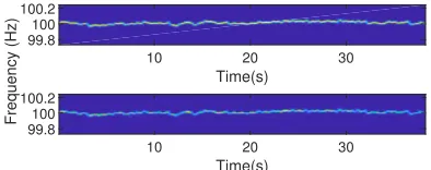
10 20 30
Time(s)
100.2 100 99.8
10 20 30
Time(s)
100.2 100 99.8
[image:4.612.348.528.81.227.2]Frequency (Hz)
Figure 2: The 2nd harmonic of the powerline EMRs sensed by an EMR sensor (upper) and a smartphone microphone (lower). The smartphone can capture the 2nd harmonic faithfully.
will generate an EMF that has a sophisticated spatial intensity distribution over the indoor space, which highly depends on the routing of the powerlines. It is thus of great interest that whether the power network EMF has the spatial distinctness and temporal stability properties desired by location sensing.
Electromagnetic emanations from building power net-works have been exploited in several applications. For in-stance, in a circuit seeker system [2], an injector injects modulated signals into a power outlet and then a seeker can identify the routing of nearby embedded powerlines by sens-ing the correspondsens-ing powerline EMR. A buildsens-ing’s power network can also be used as an effective AM radio antenna [1], because the size of a building can be close to AM radio wavelengths (i.e., hundreds meters). Different from these ex-isting applications that use the building power networks to emit certain waves, this paper inquiries whether the power network EMF, an inevitable side effect of electricity delivery, can be exploited for location sensing.
2.2
Powerline EMR Reception
We use following two techniques to sense powerline EMR.
Customized Powerline EMR Sensor:We build a power-line EMR sensor consisting of a tank circuit and a signal amplifier. Our design uses a combination of a 470 mH coil inductor and a 22µF capacitor, to achieve a resonance fre-quency of 50 Hz (i.e., the power network frefre-quency in our region). By using a 15µF capacitor, the tank circuit can be tuned to 60 Hz, which is the nominal frequency in Americas. A two-stage amplification circuit is applied to amplify the
µV-level output of the tank circuit to a volt-level input to an analog-to-digital converter mounted on a Raspberry Pi board. Our customized powerline EMR sensor can be readily integrated with various robot and drone platforms.
Side-channel Sensing by Microphone:The internal of a microphone is a capacitor consisting of a membrane and a metal conductor. The vibration of the membrane in response to sound results in time-varying capacitance between the
0 10 20 30 40 50
X (m)
0 10 20 30 40
Y (m)
[image:4.612.67.264.88.166.2]A B C D
Figure 3: Test points (A, B, C, D) and walking trajecto-ries (in thistle color) in an office building.
membrane and the metal conductor, which is translated to a voltage signal. The power network EMF can induce a time-varying voltage across the metal conductor, resulting in the mains hum in audio recordings. The mains hum can be ex-tracted using a band-pass filtering algorithm. In this paper, we use smartphones’ built-in microphones and extract the mains hum and its harmonics. Fig. 2 shows the frequency of the second harmonic sensed by a customized powerline EMR sensor and a smartphone microphone. We can see that the smartphone can capture the second harmonic faithfully.
The results based on the above two types of sensors will provide insights into the limits of power network EMF-borne spatial information and practicality of power network EMF-based location sensing on COTS mobile platforms.
3
MEASUREMENT STUDY
We conduct experiments to investigate whether the power network EMF has the properties desired for location sensing.
3.1
Power Network EMF’s Spatial
Distinctness
This set of experiments investigates whether the power net-work EMF intensities at different locations in an indoor space are distinct. We use the customized powerline EMR sensors to perform measurements in an office building with an area of about 2,475 m2. Fig. 3 shows the floor plan. We set the sampling rate of our sensors to 8 kHz and applied a 5-step moving filter to remove high-frequency noises in the sam-pled signals.
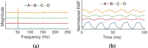
50 100 150 200 250 Frequency (Hz)
Magnitude
A B C D
(a)
0 50 100
Time (ms)
Normalized EMF
A B C D
[image:5.612.317.557.80.192.2](b)
Figure 4: Time/frequency Characteristics. (a) Power spectral density. (b)100ms signal snippets. The curves in the figures are vertically displaced for better visual comparison among them.
0 50 100 150
Distance (m)
-40 -20 0
EMF (dBFS)
158cm 173cm 188cm
(a)
0 50 100 150
Distance (m)
30 40 50 60
Magnitude (uT)
158cm 173cm 188cm
(b)
Figure 5: Power network EMF’s invariability and geo-magnetic field’s variability with user height. (a) Power network EMF. (b) Geomagnetic field.
can see that they have similar characteristics, i.e., the sensed signal consists of a 50 Hz major component and several har-monics. Fig. 4(b) shows the 100 ms snippets of the sensed signals at the four locations in the same time duration. The power network EMF intensities at different locations have distinct waveforms and amplitudes. This distinctness is con-sistent with our understanding, as power network EMF has a spatial distribution. As discussed in §2.1, this distribution mainly depends on the routing of the powerlines. As the pow-erline routing usually stays fixed, the spatially distributed power network EMF is promising for location sensing.
Invariability with User Height:The spatial distinctive-ness of indoor geomagnetic signals has been studied [8, 15]. Power network EMF and geomagnetic field are different. Ge-omagnetic field is the magnetic field that extends from the Earth’s interior out into space. Due to the metal infrastruc-ture in the buildings, geomagnetic field is distorted in indoor environments and can be utilized as the location signature. Geomagnetic intensity is static over time. In contrast, the power network EMF emitted from the ac powerlines is a time-varying field. Our following measurements show that, compared with the geomagnetic field, the power network EMF exhibits better invariability with user height.
We recruit three users with different heights (158cm, 173cm, and 188cm) who carry our powerline EMR sensor and a smartphone, and walk in a 150-meter pathway in a building.
0 10 20 30 40
Distance 0
0.1 0.2 0.3
Same Position Different Position
(a) 1-step window size.
0 100 200 300
Distance 0
0.01 0.02 0.03
*
Same Position Different Position
[image:5.612.53.294.86.164.2](b) 9-step window size.
[image:5.612.54.294.243.322.2]Figure 6: Distributions of DTW distance between two power network EMF RMS segments at the same or dif-ferent locations.
Fig. 5 shows the root mean square (RMS) value measured by our powerline EMR sensor and the geomagnetic magni-tude measured by the phone’s 3-axis magnetometer. Each RMS value is computed based on readings in a 20 ms win-dow. Though both sensing modalities are affected by the sensor altitude, the geomagnetic sensing is apparently more susceptible as the envelope of the geomagnetic magnitude varies much with user height. In contrast, the envelope of the power network EMF RMS exhibits better invariability against user height. This result implies that the power net-work EMF signature map can be constructed based on data crowd-sourced from users with different heights.
same or different locations with the observed power network EMF signals in more detail.
3.2
Power Network EMF’s Temporal
Stability
This section investigates the temporal stability of the power network EMF. Although conventional SLAM systems only require short-term stability of loop-closure landmarks, long-term stability is still desirable, because the constructed fea-ture maps can be reused for user navigation afterwards.
Impact of Individual Electric Appliances:Operating sta-tus changes of electric appliances causes varying ac currents in powerlines and therefore varying magnetic field. We con-duct a set of controlled experiments to investigate the im-pact of the on/off operating statuses of individual electric appliances on the measurements of a powerline EMR sen-sor. Fig. 10a shows the power network EMF amplitude in decibels relative to full scale (dBFS) measured at different distances from an electric appliance when it is on and off. We can see that the operating statuses of the appliances can affect the power network EMF measurements. However, the impact is less than 1 dBFS when the sensor is more than one meter from the appliance. This is because that the magnetic intensity attenuates with distance and the measurement of the sensor is dominated by the superposition of the EMRs from all powerlines in the building compared with the EMR contributed by the tested appliance. Among the eight tested appliances, the operating status changes of the dryer, the microwave, and the fridge introduce considerable impact on the sensor measurements in their near fields. However, the near fields of these appliances are generally limited com-pared with the walking areas of built environments. From the measurement results, we can observe that switching off some appliances may increase the measurements at certain distances. This is because these appliances make negative contributions to the EMR superposition at those distances.
Impact of Near-by Human Bodies:A researcher holds a powerline EMR sensor and stands still at an indoor loca-tion. Then, more persons join the experiment by standing still about 0.5 m from the researcher. Fig. 8 shows the error bars of the sensor measurements when different numbers of persons stand around the researcher. We can see that the nearby human bodies have little impact on the sensor measurements. Unlike the short-wavelength RF signals (e.g., WiFi) that are susceptible to barriers, the 50 Hz EMR signal has an extremely long wavelength and thus are not affected by small-size barriers like human bodies.
Temporal Stability:We deploy four customized powerline EMR sensors at four different fixed locations in two countries
for 14 days. Each sensor records power network EMF inten-sities for one minute every two hours. Fig. 10a shows the error bars of each sensor’s measurements in the one-minute duration. We can see that their measurements are stable over time. For comparison, Fig. 9 shows a smartphone’s WiFi RSS values for a number of access points over 24 hours. We can clearly see the temporal variations of the WiFi RSS.
We also measure the power network EMF intensity when traversing a loop along the trajectory shown in Fig. 3 in a winter and the following summer. Fig. 10b plots the power network EMF RMS traces in the two seasons. As the building shown in Fig. 3 is located in the Temperate Zone, the electric loadings of the building in winter and summer are differ-ent. However, as shown in Fig. 10b, the power network EMF traces in the two seasons are desirably similar. This suggests that the ac voltage is the major exciter of the power network EMF, rather than the loading-dependent current. The above results show the power network EMF’s temporal stability in the tested sites, and imply that once a power network EMF fingerprint database is developed through SLAM, it can be used for localization in considerably long time periods. In case of building infrastructure changes and/or powerline rerouting, it is readily for existing crowd-sourcing localiza-tion tools to update the database timely.
3.3
Location Discriminability of Power
Network EMF Sensed by Smartphone
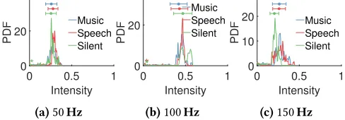
Phone’s Power Network EMF Sensing Performance:As microphone is a side-channel sensor, we assess the impact of various daily life sounds on its power network EMF sensing. A Huawei P9 phone is placed at a fixed location to record audio for five minutes. Meanwhile, we intentionally create various interfering sounds, i.e., music and human speech that are most probably faced by SLAM/localization systems for pedestrians. Fig. 11 shows the distributions of the normalized intensity of the 50 Hz mains hum and its harmonics. From the figure, we can see that the music and human speech have larger impact on the 150 Hz harmonic, compared with the 50 Hz mains hum and the 100 Hz harmonic. This is because the 150 Hz harmonic collides with some human voice com-ponents. Although human voice can be down to 80 Hz [32] and collides with the 100 Hz harmonic, such cases are rare. As some high-end phones can effectively suppress the 50 Hz mains hum, we adopt the 100 Hz harmonic only, unless we need multiple harmonics to improve performance (cf. §4.4).
Mitigating Inefficacy of Geomagnetism-based Sensing:
40 80 120 160 Distance (cm) -22 -20 -18 -16
EMF (dBFS) on off
(a) Boiler
40 80 120 160
Distance (cm) -19 -18 -17 -16 -15 EMF (dBFS) on off (b) Computer
40 80 120 160
Distance (cm) -22 -20 -18 -16 -14 EMF (dBFS) on off
(c) Hair dryer
40 80 120 160
Distance (cm) -30 -25 -20 -15 EMF (dBFS) on off
(d) Fluorescent light
40 80 120 160
Distance (cm) -30 -20 -10 EMF (dBFS) on off (e) Microwave
40 80 120 160
Distance (cm) -65 -60 -55 -50 EMF (dBFS) on off
(f) Computer monitor
40 80 120 160
Distance (cm) -25 -20 -15 EMF (dBFS) on off
(g) Air purifier
40 80 120 160
[image:7.612.54.559.83.265.2]Distance (cm) -22 -20 -18 -16 EMF (dBFS) on off (h) Fridge
Figure 7: Impact of individual electric appliances on power network EMF sensing.
[image:7.612.316.560.302.387.2]Scenario -20 -18 -16 -14 EMF (dBFS) handheld 1 person 2 persons 3 persons
Figure 8: Nearby human body impact.
4 8 12 16 20 24
Time (hour) 1 2 3 4 5 6 7 8 Access Point -100 -90 -80 -70 -60 RSS(dB)
Figure 9: Temporal varia-tion of WiFi RSS.
0 100 200 300
Time (h) -30 -20 -10 EMF (dBFS) P
1 P2 P3 P4
(a)
0 100 200 300
Distance (m) -30 -20 -10 EMF (dBFS) winter summer (b)
Figure 10: Temporal stability. (a) The power network EMF amplitude measured at four fixed locations in two countries over 14 days. The measurements labeled byP1andP2are obtained in country A; these labeled by
P3andP4are obtained in country B. (b) The power net-work EMF amplitude trace when a researcher carrying the sensor walks along the same trajectory shown in Fig. 3 in a winter and the following summer.
particularly investigates the feasibility of using microphone-sensed EMF to mitigate the localization inefficient points by geomagnetic sensing. The insight for the mitigation is that when geomagnetic features are less discriminative (small gap) and insufficient to differentiate locations, power net-work EMF sensing can help enhance location distinctions,
0 0.5 1
Intensity 0 20 PDF * Music Speech Silent
(a)50Hz
0 0.5 1
Intensity 0 20 PDF * * * Music Speech Silent
(b)100Hz
0 0.5 1
Intensity 0 10 20 PDF Music Speech Silent
(c)150Hz
Figure 11: Power network EMF captured by a smart-phone microsmart-phone.
0 10 20 30
Distance 0 0.05 0.1 0.15 PDF Mag micEMR Mag+micEMR
(a) Same location
0 10 20 30
Distance 0 1 2 3 PDF Mag micEMR Mag+micEMR
(b) Different locations
Figure 12: DTW distance distributions of various modalities at the same and different locations.
Features location
EMF1 (x1,y1)
EMF2 (x2,y2)
EMF3 (x3,y3)
Odometry
EMF Sensing
EMF SLAM
EMF Extraction
Segmentation
Loop Closure Detection
Loop Closure Curation
Graph Optimization
EMF Localization
Feature Extraction
[image:8.612.65.277.88.214.2]Effiicient Feat. Matching
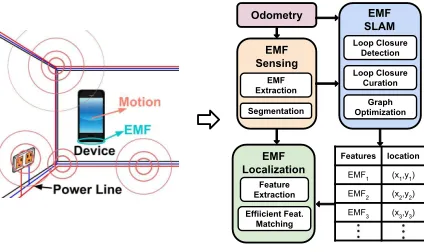
Figure 13: System workflow.
undermining the recall and precision performance in loca-tion identificaloca-tion. The curves labeled “micEMR” are the corresponding results obtained using the 100 Hz powerline EMR harmonic sensed by the P9’s microphone. Although the micEMR’s two distributions overlap, the micEMR’s recall and precision performance will be clearly better than the geomagnetism’s. The “Mag+micEMR” curves are the corre-sponding results using the average of the Mag-based and micEMR-based DTW distances. The above results show that, on smartphone platforms, power network EMF and geomag-netism can be complementary in discriminating locations. A combination of geomagnetism and power network EMF can mitigate inefficacy of sole geomagnetism-based location sensing.
Power Consumption of Power Network EMF Sensing:
According to the study [40], the power consumption of sam-pling microphone is low. On the other hand, the plethora of acoustic-based virtual assists on smartphones and wearables (e.g., Apple Siri [37]) also require the microphones to be al-ways on. Therefore, in practice, our proposed approach can leverage the audio data collected by these virtual assistants, without incurring excessive energy consumption.
4
SLAM WITH POWER NETWORK EMF
Based on the understanding obtained in §3, this section devel-ops a novelSimultaneousLocalizationAndMapping (SLAM) approach with the power network EMF. As discuss above, power network EMF tends to exhibit better temporal sta-bility comparing to geomagnetism, while providing certain spatial discriminability. However unlike other modalities such as vision, loop closures candidates obtained by directly comparing the power network EMF signal similarities of-ten contain many false positives, which could significantly degrade the SLAM performance. To address this, the pro-posed SLAM approach employs novel loop closure detection and curation algorithms, which are able to discover as many potential loop closures as possible based on the sequential power network EMF measurements, while robustly rejecting
I
C0,3
x
0 x1 x2 x3 ...
u 1
z
0 z3
u
2 u3
Figure 14: Factor graph representation for EMF-SLAM. xis the hidden state of actual user position;zdenotes the power network EMF measurement; cis the loop closure of same place.
the false positive loop closure proposals by checking their spatial consistency.
Fig. 13 illustrates the workflow of our SLAM and local-ization approaches. Specifically, the sensed power network EMF signals are bandpass-filtered to extract the 50/60Hz sig-nal and its harmonics. By using a dead-reckoning module on the motion data of the user, her trajectories/odometry is estimated. The filtered power network EMF signal is then segmented into sequences based on footsteps estimated in odometry information. The power network EMF sequences and odometry are sent to the loop closure detection module to first detect the revisited positions by the user. The detected loop closures are then curated to remove false positives in them. By using the SLAM algorithms with the estimated odometry and curated loop closures, the accurate trajecto-ries of users can be recovered. By looking back the timestamp of the recovered locations and their associated power net-work EMF signatures, a feature map can be constructed. New users’ location can be predicted via matching their power network EMF readings with the feature map, even if their odometry information is not available. Note that this SLAM approach is fundamentally different from the standard fin-gerprinting. In our case, the feature map is automatically constructed as users move across the space, rather than man-ually collected through the labor-intensive fingerprinting process, which requires the users to explicitly establish the correspondence between specific locations and their EMF features. In addition, our SLAM approach can continuously improve and enrich the EMF feature map as the users ex-plore the space more, e.g. in different walking directions, and eventually obtain a holistic view of the EMF signatures of the environment.
4.1
Graph SLAM Formulation
States, Measurements and Outputs: Fig. 14 shows the factor graph representation of our SLAM formulation. Letxt
denote the hiddenstate, i.e., actual position of the user in the workspace at discrete timestampt. We assume that at each
t, the user observes apower network EMF measurementzt, which contains the sequence of power network EMF signals received within a window [t−τ,t]. Note that here we con-sider a signal sequence rather than point as the measurement because as shown in §3.1, longer power network EMF signal sequences tend to have more spatial discriminative power. We also assume that the relative displacement between two user positionsxt andxt−1is captured by an odometry edge ut, e.g., estimated with PDR techniques. In practice, we often assume the initial location of the user (starting stateI) can be known through other sources [26], e.g., CCTVs or card swipe systems at the entrance of the venue. After the user finishes traversing the workspace, the SLAM module should output the estimated sequence of true locations of the userx0, ...,xT,
along with the power network EMF feature map, which can be obtained by associating the observed power network EMF measurementsz0, ...,zT with the state sequence.
Loop Closure using Power Network EMF Signals: In a typical SLAM setting, loop closure refers to the recognition of when the user or agent has returned to a previously vis-ited location, e.g., via observing similar measurements. It is one of the key components of SLAM framework, since in most cases, odometry measurements tend to be noisy, result-ing in unbounded errors in state and map estimation. For instance, our system uses a PDR module which relies on the low-cost IMUs on mobile devices to estimate odometry, and inherently suffers from drift. Loop closure on the other hand, can enforce constraints (often on distance) between states, e.g.,x0andx3in Fig. 14 are connected by an edgec0,3,
indi-cating that they should represent the same location in the workspace. This immediately reduces the uncertainty in state and map estimation, and therefore, the quality of detected loop closures has a direct impact on SLAM performance. In this work, we exploit the similarity between features at 50Hz of the observed power network EMF measurements to detect loop closures. As shown later, by carefully designing detection and curation algorithms, the power network EMF signals can be used to generate effective and robust loop closures across the workspace.
Graph Optimization: Given the odometry and loop clo-sures, the optimal state sequenceX∗={x∗
0, ...,xT∗}can be
estimated by solving:
X∗=argmin
X X
i
||fu(xi,ui)−xi+1||Σ2i
| {z } odometry constraints
+X
<i,j>
||fc(xi,cij)−xj||2Λ i j | {z } EMF loop closure constraints
Timestamp Closest-pointtimestamp Closest-pointdistance
1 42 0.94
24 129 0.21
58 280 0.25
129 231 0.18
231 129 0.18
280 58 0.25
(a) CPP
#129 #231
#24
#24 #129
#231
[image:9.612.328.546.80.202.2](b) Proposal merging
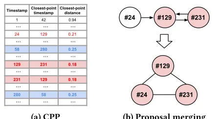
Figure 15: Illustration example of closest-point profile (CPP) and loop-closing proposals. (a) Color-shaded fields are primary loop closures and the transparent field is a subsidiary one. (b) Merging primary and sub-sidiary loop-closing proposals. Nodes in the graph are proposal nodes, and edges are proposed loop closures.
wherefu(xi,ui)describes the user motion reported by odome-tery, with uncertainty characterized by covariance matrix
Σi.fc(xi,cij)is the loop closure model, and in this paper we use co-location with zero displacement, i.e.,fc(xi,cij)=xj, and the covariance isΛij.
4.2
Loop Closure Detection
This section presents the proposed approach of detecting loop closures using power network EMF signals.
Distance between Measurements: One key prerequisite for any loop closure approach is the distance metric between the measurements. In our context, a power network EMF measurement contains a sequence of power network EMF signals. To account for different walking speed of the users, when comparing two measurementszt andzt′, we use
dy-namic time warping (DTW) to align them, i.e. we first stretch the two sequences and then use the smallest sum of the Eu-clidean distances between their corresponding points as the distance metric. For each newly observed measurementzt, we compute its distance with respect to all previous measure-ments, and maintain the pairwise distance between them in a matrixQ.
Closest Point Profile (CPP): Given the currentQ, we try to discover loop closures, i.e., measurements that are similar to each other and likely to represent the same locations. In-stead of directly working withQ, we firstly derive aclosest point profile(CPP) representation, where for each measure-ment we only keep the timestamp of its closest peer and their distance. For instance, the entry (129, 213, 0.18) in Fig. 15 means that for measurementz129, the closest measurement
(i.e., most similar one) observed so far isz231, and their
x y
PASS FAIL
x y
x y
Ti
Tj Ti
Tj
x y
Initial pose
Final
pose Initial pose
Final
pose Tj
Tj
Ti with
inverse odometry
zv
Ti with
inverse odometry
zv
zv’
zu
zu z
u’
zu
zv(z )v’ zv(z )v’
zu’
zu’
zv’
zr’ zr
(a) Spatial consistency validation.
Ti
Tj
zv’
zv
zu’
zu
UPDATE Ti
Tj
zv’
zv
zu’
zu
[image:10.612.65.286.78.292.2](b) Distance update induced by validation.
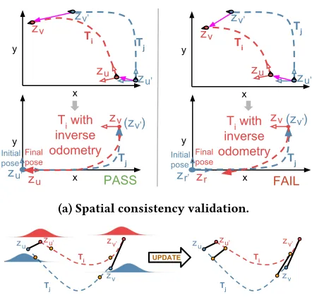
Figure 16: An example of loop closure curation.
that, in practice, CPP may not necessarily be symmetric un-der the distance metric. For example, as in Fig. 15, the closest peer ofz24isz129, but forz129,z24is not the closest.
Mining Loop Closure Proposals from CPP: Intuitively, the entries in CPP are potential loop closures, each of which represents the local best knowledge on closest measurements and associated distances. Like most of the existing SLAM approaches, we could just naively threshold the distance, and propose the top-kentries with smallest distances as loop closures. However, in practice, such a technique is not ro-bust to noise, and could propose many false positives. In this paper, we consider a new approach exploiting the graph structure of CPP. Concretely, we first discover the symmetric entries within CPP, e.g., as shown in Fig. 15, bothz129and z231treat each other as the closest peer. The rationale is that,
regardless of the absolute distances, the fact that both mea-surements confirm each other as the closest indicates that they are likely to observe the same landmark. Therefore, we initialize the set of loop closure proposals using those sym-metric entries. To harvest more potential loop closures, we also add entries whose 2-nearest neighbours are symmetric, e.g., entry (24, 129, 0.21) in Fig. 15(b) will be included in the loop closure proposal set, since measurementz129appears
in an symmetric entry.
4.3
Loop Closure Curation
Given the set of loop closure proposals, in theory, we could use all of them to directly optimize the graph and solve the SLAM problem (as in §4.1). However, in practice, the SLAM framework can be very sensitive to false positives,
i.e., even a small amount of erroneous loop closures would greatly deteriorate graph optimization, and have a knock-on effect knock-on its performance. To address this, we propose a loop closure curation approach, and exploit the spatial consistency to reject false positives and iteratively discover new valid proposals.
Spatial Consistency Validation: In our context, a true loop closure contains a pair of measurements which observe the same landmark in the workspace, although they may be captured at different timestamps or even by different users. Consider two loop closure proposals, involving two pair of measurements as (zu,z(u′) andzv,zv′) as shown in
Fig. 16a(left). In this case, if both loop closures are true, then within any consistent reference frame, the two trajectory segmentsTi andTjdefined by the four measurements will form aloop, sincezu andzu′,zvandzv′should be observed
in the same locations. Consider the 2D Euclidean reference frame wherezu′is positioned at the origin (0, 0).
Concep-tually, if we move fromzu′(at the origin) tozv′using the
odometry information encoded inTj, hop tozvvia the loop
closure link fromzv′, and then traverse back according to
thereverseodometry inTi, when reaching measurementzu
we should be able to return to the origin. This is becausezu
andzu′should correspond to the same landmark. If this is
the case, we confirm that both loop closure proposals are true, and mark them as valid (ready to be used by the later graph optimization). On the other hand, if we fail to return to the origin, e.g., as shown in Fig. 16a(right), then at least one of the two loop closure proposals is false positive. In that case we will not push any of them to later optimiza-tion, and temporarily keep them in the proposal set for next validation.
Distance Update Induced by Validation: As discussed above, if two loop closure proposals pass the the spatial consistency validation, we believe that the two trajectory segments (seeTi andTj in Fig. 16b) would share the same start and end locations in the workspace (zu andzu′,zvand zv′in Fig. 16a(left)). On the other hand, this also indicates
that measurements within the neighbourhood of those vali-dated loop closures should be spatially close, and there might still be valid loop closures missed by the previous detection algorithm. To exploit this constraint, we update the pairwise distances of those measurements within that neighborhood.
Concretely, given the validated loop closure containing two measurementszu andzu′ (zu ∈Ti,zu′ ∈Tj), we first
consider the neighborhood of 2N +1 measurements around
zu andzu′respectively, i.e., two sequences of measurements {zu−N, ...,zu+N}and{zu′−N, ...,zu′+N}. The size ofN is
de-termined by the shape similarity of the two trajectory seg-mentsTi andTj:N ∝ 1/DTW(Ti,Tj), whereDTW(Ti,Tj)
Lab Space Office Building
Shopping Mall (Indoor)
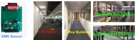
[image:11.612.65.282.84.149.2]Shopping Mall (Outdoor) EMR Sensor
Figure 17: Powerline EMR sensor and test venues.
the 2N +1 window, we define a Gaussian kernel:w(n) =
e−12(Q(zu,zu′)·Nn)2, where−N ≤n ≤N, andQ(z
u,zu′)is the
distance between measurementszuandzu′of the validated
loop closure. Then for each pair of measurementszu+n ∈Ti
andzu′+n′ ∈Tj (−N ≤n,n′≤N) between the two 2N+1
windows, we update their distance as follows:
Qnew(zu+n,zu′+n′)=Q(zu+n,zu′+n′)−β·w(n)·Q(zu,zu′).
Here,Q(zu+n,zu′+n′) is the current distance, and β is the
updating rate which controls how much distance change should be applied.
Iterative Loop Closure Curation: With the updatedQ, where measurements around the validated loop closures have new distance values, we then drive the detection al-gorithm to discover any new loop closure proposals. This detection-validation cycle runs iteratively: in each iteration we first discover loop closure proposals, validate them, and finally use the validation results as constraints to update our previous belief on distances between measurements, which is then used by the loop closure detection algorithm in the next iteration. This loop closure curation process continues, until there is no proposal can satisfy the spatial consistency validation. In this way, our system is able to discover as many genuine loop closures as possible, and as shown later in the evaluation, it is the key for our SLAM framework to build accurate and consistent power network EMF feature maps.
4.4
Efficient Real-time Localization
In essence, the proposed SLAM framework leverages the odometry information and power network EMF, to jointly estimate the location of the user and the power network EMF feature map of the workspace within a metrically consistent frame of reference. In practice, this process typically hap-pens offline in the cloud, since it requires optimization over all states and measurements (as discussed in §4.1). On the other hand, if the power network EMF feature map of the workspace has been constructed using the proposed SLAM approach (e.g., via crowdsourcing), we could position the user directly with respect to the map. In the following, we show that such localization can be achieved in real-time on resource-constrained devices without infrastructure support: once the power network EMF feature map is downloaded
to the user’s mobile device, she can be localized using the carried device only.
Localization with Power Network EMF Feature Map:
Assume that the workspace is a 2DdiscreteEuclidean space, and has been thoroughly surveyed by our SLAM approach. In this case, the produced power network EMF feature map can be viewed as a 2D grid, where each grid represents a location
land the associated power network EMF signature ¯zl. In this
paper, ¯zlis defined as the DTW centroid [30, 31] of all power network EMF measurements observed at locationl, which is also a sequence of power network EMF signals. Therefore, localization with respect to the feature map can be cast into a classification problem, where for a live power network EMF measurementzt, we try to find the location that has the closest power network EMF signature. In our context, we consider a similar distance metric as in §4.2, which employs DTW to evaluate the similarity between power network EMF signal sequences. However, unlike in SLAM (see §4.2) where we only use power network EMF features at 50 Hz for ro-bustness, during localization we consider three frequency components 50 Hz, 100 Hz and 150 Hz (the harmonics), to exploit more discriminative power of power network EMF signals. Therefore, the distance between the live power net-work EMF measurement zt and the power network EMF signature at a given location is evaluated as the weighted sum of distances between signals at the three frequency com-ponents, where weights are learned from the data. Finally, given the pairwise distances between live power network EMF measurementzt and power network EMF signatures at different locations, the estimated location is given by a Nearest Neighbour (NN) classifier.
Sparse Power Network EMF Feature Analysis:The above localization scheme is intuitive and easy to implement, but may incur substantial computational cost since a newly ob-served power network EMF measurement has to be com-pared against power network EMF signatures of all locations within the feature map, where each comparison involves one run of DTW. This would pose significant negative effect on performance when feature maps become bigger/denser, or for resource constrained devices such as wearables. To address this, we propose a sparse power network EMF fea-ture analysis approach which only works on much sparser power network EMF signals to speed up processing. The intuition is that within a short period, the power network EMF signals tend tosmoothwith low variance, i.e., most val-ues are entered around the sample mean. Therefore, when comparing a given measurementztwith the power network
EMF signatures in the feature map, we first use the mean values to filter out those locations whose mean power net-work EMF signatures are very far away from that ofzt. In
our experiments, we find that this pre-processing step is very
0 10 20 X (m) -15
-10 -5 0 5 10 15
Y (m)
0 10 20
X (m) -5
0 5 10 15
Y (m)
GroundTruth senEMR
0 10 20
X (m) -5
0 5 10 15
Y (m)
GroundTruth micEMR+Mag
-20 0 20 40
X (m) -40
-20 0 20 40
Y (m)
-20 -10 0
X (m) -20
-10 0 10 20
Y (m)
GroundTruth senEMR
-20 -10 0 X (m) -20
-10 0 10 20
Y (m)
GroundTruth micEMR+Mag
(a) Floorplans.
-100 0 100 200 X (m) 0
50 100
Y (m)
(b) Inertial trajectories.
0 50 100 150
X (m) 0
20 40 60
Y (m)
GroundTruth senEMR
(c) senEMR-SLAM.
0 50 100 150 X (m) 0
20 40 60
Y (m)
GroundTruth micEMR+Mag
[image:12.612.57.557.78.358.2](d) micEMR+Mag-SLAM.
Figure 18: Floorplans (a), inertial trajectories produced by PDR (b), and the maps estimated by the proposed senEMR-SLAM (c) and micEMR+Mag-SLAM (d) in lab (top), office building (middle) and shopping mall (down).
effective: on average it can rule out about 90% of locations in the feature map, with less than 2% drop in overall local-ization accuracy. In addition, given the sample meanµ(zt)
and varianceσ(zt)of a power network EMF measurement
zt, the signal sequence encoded inzt can be sparsified by collapsing all values within [µ(zt)−λσ(zt),µ(zt)+λσ(zt)] as zeros.λis the sparsity factor, which controls how much information would be omitted from the original signal. The resulting consecutive zeros are then clustered together, and we only keep the lengths of them in the sequence. We apply the same process to the power network EMF signatures, and then run DTW on the sparse representations, which should be much shorter than the original signals. The rationale is that we have already used mean values to comparezt with
the power network EMF signatures, and thus values close to its mean won’t be able to contribute further information. As shown later in the evaluation, this sparse analysis approach can significantly reduce computation latency of localization.
5
EVALUATION
5.1
Experiment Setup
Sites: We evaluated the performance of proposed power net-work EMF-based SLAM and localization approaches in three venues across two countries, including (i) an office building
(1,750 m2), which was built over 20 years ago with stones and
bricks, and reinforced with metal rebars; (ii) a semi-outdoor shopping center (11,000 m2) built recently close to a high-way; and (iii) a lab space (900 m2) in another country, which has the same 50Hz powerline frequency but different layout. Fig. 17 shows the snapshots of these test venues.
Sensing Modalities and Platforms: In our experiments we employed a variety of sensing modalities, and collected the following data: (i) power network EMF signals from a cus-tomized powerline EMR sensor as shown in Fig. 17, (ii) audio from microphones, (iii) geomagnetic field from the smart-phone magnetometer, and (iv) WiFi RSS on smartsmart-phones. We used 5 devices with different specs, including Raspberry Pi 2 and 3, Galaxy S7, Huawei P9, and Nexus 6.
0 2 4 6 8 Error (m)
0 0.2 0.4 0.6 0.8 1
CDF
senEMR micEMR Mag WiFi micEMR+Mag micEMR+WiFi
(a) Sensing modality
0 2 4 6
Error (m) 0
0.2 0.4 0.6 0.8 1
CDF
Proposed Vertigo Max-Mixture RRR NoValidation
[image:13.612.56.294.81.177.2](b) Validation method
Figure 19: SLAM performance in the lab space.
5.2
Experiment Results
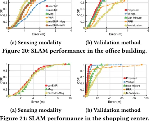
Effectiveness of SLAM using Power Network EMF:The first experiment studies the effectiveness of SLAM using power network EMF. We refer to the SLAM approach using power network EMF sensed via the customized receiver as senEMR-SLAM, while via microphone asmicEMR-SLAM. The two proposed approaches are compared against: (i) WiFi-SLAMand (ii)Mag-SLAM, which use WiFi RSS [11, 50] and earth geomagnetic field [12, 44] for SLAM. Fig. 18 shows the floorplans (a), the inertial trajectories produced by PDR (b), and the maps (shown as trajectories) estimated by the proposed senEMR-SLAM (c) and micEMR+Mag-SLAM (d) across three experiment sites. We see that in all sites both ap-proaches can produce much more consistent trajectories than PDR, which are very similar to the ground truth. Fig. 19(a), 20(a) and 21(a) further show the error distributions of maps constructed by different SLAM approaches using a variety of sensing modalities. As we can see, senEMR-SLAM con-sistently outperforms the other single-modality SLAM ap-proaches, and can reach 0.42m accuracy for 90% of the time in the lab space, while achieving 3.34m mean accuracy in the very challenging shopping center. On the other hand, Mag-SLAM has about 15% more error than senEMR-Mag-SLAM, while WiFi-SLAM performs even worse. Although both exploit the power network EMF, the performance of micEMR-SLAM is generally inferior to senEMR-SLAM due to the background noise in audio data. This is expected, however in the lab space micEMR-SLAM is still better than WiFi-SLAM (Fig. 19(a)). In the challenging shopping center, neither micEMR-SLAM nor WiFi-SLAM is able to construct a reasonable map (errors not shown in Fig. 21(a)). On the other hand, when fused with other sensing modalities, e.g. micEMR-SLAM + Mag-SLAM, the SLAM accuracy could improve by 20% on average than Mag-SLAM alone.
Performance of Iterative Loop Closure Curation:This experiment investigates the performance of the proposed iterative loop closure curation algorithm. We compare our approach with the state-of-the-art loop closure checking algorithms: (i)RRR[21] which identifies valid loop closures by clustering them; (ii)Max-mixture[28] which employs a mixture model to capture probabilities of valid loop closures;
0 1 2 3 4
Error (m) 0
0.2 0.4 0.6 0.8 1
CDF
senEMR micEMR Mag WiFi micEMR+Mag micEMR+WiFi
(a) Sensing modality
0 2 4 6
Error (m) 0
0.2 0.4 0.6 0.8 1
CDF
Proposed Vertigo Max-Mixture RRR NoValidation
[image:13.612.318.558.92.287.2](b) Validation method
Figure 20: SLAM performance in the office building.
0 2 4 6 8 10
Error (m) 0
0.2 0.4 0.6 0.8 1
CDF
senEMR Mag micEMR+Mag
(a) Sensing modality
0 20 40 60 80 100
Error (m) 0
0.2 0.4 0.6 0.8 1
CDF
Proposed Vertigo Max-Mixture RRR NoValidation
[image:13.612.317.560.194.287.2](b) Validation method
Figure 21: SLAM performance in the shopping center.
and (iii)Vertigo[39], which uses latent variables to model the validity of loop closures. We also include the baselineNo Validation, which naively pushes all loop closure proposals to optimization without any validation. Fig. 19(b), 20(b) and 21(b) shows the error CDF of different approaches. Firstly, we see that loop closure validation is a necessary step, and can significantly improve SLAM accuracy: in the shopping center, the proposed approach can reduce the error to 20% (from 15.06m to 3.34m), compared to no validation. Comparing to other loop closure validation techniques, our approach can achieve approximately 1.5-fold reduction in error and the accuracy degrades gracefully. This is because our approach is able to iteratively validate and mine genuine loop closures, while the competing ones just run one-off validation.
0 5 10 15 20 25 Error (m)
0 0.2 0.4 0.6 0.8 1
CDF senEMR
micEMR Mag micEMR+Mag
(a) Lab space
0 10 20 30 40
Error (m) 0
0.2 0.4 0.6 0.8 1
CDF senEMR
micEMR Mag micEMR+Mag
[image:14.612.337.542.81.158.2](b) Office building
Figure 22: Localization performance of different sens-ing modalities.
a participant of height 162cm to build the magnetic feature map, while tried to localise another of 190cm. This confirms that magnetism based approaches are not robust to height, while the proposed power network EMF based approaches do not suffer from this problem. On the other hand, using only power network EMF sensed via microphones (micEMR-Loc) has generally larger errors than that of using customized receivers (senEMR-Loc). However, when fused with mag-netic field (micEMR+Mag-Loc), the localization errors could be halved comparing to the single best modality: from 8.2m (micEMR-Loc only) to 3.7m in the lab space and 8.4m (Mag-Loc only) to 3.9m in the office building.
Sensitivity to Power Network EMF Sequence Length:
This experiment looks into the sensitivity of localization per-formance with respect to the sequence length of power net-work EMF signals included in one measurement. We consider two realistic settings: (i) running senEMR-Loc on Raspberry Pi (RP2 and RP3), which can be used in various IoT applica-tions; and (ii) running micEMR+Mag-Loc (fusion of micEMR-Loc and Mag-micEMR-Loc) on smartphones, which provides an alter-native option for infrastructure-free positioning. As shown in Fig. 24 and 25, we vary the length of power network EMF sig-nals in terms of steps: e.g. 2-step means in a power network EMF measurement we include signals observed within the last 2 steps. We see that senEMR-Loc and micEMR+Mag-Loc achieve comparable localization accuracy: generally longer sequences result in better accuracy, while the gaps become marginal when the sequence length is bigger than 6-step. For instance, for both senEMR-Loc and micEMR+Mag-Loc, using signals of 10-step would only improve localization ac-curacy by<0.2m comparing to 6-step. On the other hand, longer sequences take more time to process, e.g. using 10-step would significantly increase localization time as shown in Fig. 24 and 25 (up to∼3s for one measurement), which is not cost-effective.
Performance Gain by Sparse Feature Analysis:The last set of experiments verify the impact of the proposed sparse feature analysis on localization performance. We use the same two settings (that is, senEMR-Loc on Raspberry Pi, and
25.11X 21.12X 20.56X 20.60X
Huawei Nexus RP2 RP3
0 10 20
Time (s)
[image:14.612.52.298.82.166.2]standard constrained mean filter(proposed) full-suite(proposed)
Figure 23: Running time of different feature analysis approaches on test devices.
Table 1: Localization accuracy (m) of different feature analysis approaches.
raw DTW constrained mean filter full senEMR 1.76 1.89 1.77 2.01 micEMR
+ Mag 4.15 5.58 4.20 4.71
0 0 10
Error (m)
5
20 1
Sparsity Level(%)
30 3
Steps
40 5
7
50 9
(a) Error
0 0 2
10
Time (s)
20 4
Sparsity Level(%)
9
30 7
Steps
40 5
50 1 3
[image:15.612.55.294.82.333.2](b) Running time
Figure 24: Accuracy and running time on RP3.
0 0 10
Error (m)
5
20 1
Sparsity Level(%)
30 3
Steps
40 7 5
50 9
(a) Error
0 0
Time (s)
10 0.5
20
Sparsity Level(%)
9
30 7
Steps
40 5
50 1 3
[image:15.612.56.297.86.194.2](b) Running time
Figure 25: Accuracy and running time on Huawei P9.
6
RELATED WORK
As discussed in §1, recent studies [23, 33, 48] have exploited powerline EMR for time-related services. In [29, 38], mod-ulated high-frequency signals are injected into a building’s power network and then the corresponding power network emanations are sensed by a mobile device equipped with an EMR sensor for localization. However, the requirements of one or more signal injectors and intensivein situtraining introduce significant system deployment overhead. The Hu-mantenna system presented in [9] uses the human body as an antenna to receive powerline EMR and recognize gestures. Preliminary results on recognizing the user’s location among pre-spotted locations are presented. However, the physical connection with the user’s body and system training bring overheads. To the best of our knowledge, this paper presents the first work on using power network ENF measurements captured by a standalone sensor or smartphone for SLAM and localization.
Originally designed for robotics, SLAM has been applied to mobile computing applications [3, 43]. However, due to mobile devices’ low-cost and noisy IMUs and human’s com-plicated motion patterns, SLAM for human-centric applica-tions is often challenging. Early solution [11, 50] use WiFi RSS and IMUs for SLAM. However, WiFi RSS suffers from the multi-path effects and the performance of SLAM de-grades significantly in dynamic environments, e.g., retail stores. Geomagnetism-based SLAM is recently introduced [12, 18, 44]. However, geomagnetism often exhibits high
variability with altitude. Recent SLAM systems also leverage vision techniques [10, 14], which raise privacy concerns [52], however. Our SLAM system differs from the above systems in its new sensing modality – power network EMF – that ex-hibits desirable high repeatability. Our system also features a bespoke approach that detects power network EMF loop closures reliably and produces better SLAM results.
Localization can be seen as a special case of SLAM where the map is known or obtained through SLAM. Existing local-ization approaches can be divided into two categories. First, model-basedapproaches estimate the distance between a user device and deployed anchors based on models of RSS [5, 7], angle of arrival [20, 46], or propagation time [25, 42, 45]. However, non-line-of-sight conditions often degrade the per-formance of these approaches. Differently, powerline EMR with extremely long wavelengths can well penetrate bar-riers. Second,fingerprintingapproaches develop a map of features extracted from images [13, 54], sounds [41], geo-magnetic field [22, 35, 36], RF signals [6, 51], visible lights [49, 52, 55] and a mix of them [4, 34, 47]. However, these approaches generally require a laborious blanket process of (re-)fingerprinting all locations. Owing to the temporal stability of power network EMF, our approach requires a one-shot profiling only, coinciding with the concept oflight registration[53]. Moreover, the profiling can be accomplished via crowd-sourced SLAM in an unsupervised manner.
7
CONCLUSION
This paper systematically investigated the spatial distinct-ness and temporal stability of EMFs induced by buildings’ power networks. Based on the result, we designed a SLAM ap-proach that can reliably detect loop closures with power net-work EMF signals sensed by either a customized receiver or a smartphone’s microphone as a side-channel sensor. More-over, with the power network EMF feature map constructed by SLAM, we design an efficient localization algorithm that can position the user in real time on resource-constrained devices. Our extensive evaluation shows that the power net-work EMF is a promising modality for indoor location sens-ing since it is ubiquitous, spatially distinct, temporally sta-ble, and noise resilient. By exploiting these advantages of power network EMF, the proposed SLAM and localization approaches are capable of achieving sub-meter accuracy, while run in real time on both smartphones and embedded hardware. Advanced approaches for fusing power network EMF measurements with the measurements in other sens-ing modalities, as well as 3D indoor localization with power network EMF are interesting topics for future work.
REFERENCES
[1] [n. d.]. Carrier Current Radio Systems. ([n. d.]). http://www. radiosystems.com/carriercurrent.html.
[2] [n. d.]. Greenlee Circuit Seeker. ([n. d.]). http://bit.ly/2tzf6EI. [3] Heba Abdelnasser, Reham Mohamed, Ahmed Elgohary, Moustafa Farid
Alzantot, He Wang, Souvik Sen, Romit Roy Choudhury, and Moustafa Youssef. 2016. SemanticSLAM: Using environment landmarks for un-supervised indoor localization.IEEE Transactions on Mobile Computing
(2016).
[4] Martin Azizyan, Ionut Constandache, and Romit Roy Choudhury. 2009. SurroundSense: mobile phone localization via ambience fingerprinting. InACM MobiCom.
[5] Paramvir Bahl and Venkata N Padmanabhan. 2000. RADAR: An in-building RF-based user location and tracking system. InIEEE INFO-COM.
[6] Yin Chen, Dimitrios Lymberopoulos, Jie Liu, and Bodhi Priyantha. 2012. Fm-based indoor localization. InACM MobiSys.
[7] Krishna Chintalapudi, Anand Padmanabha Iyer, and Venkata N Pad-manabhan. 2010. Indoor localization without the pain. InACM Mobi-Com.
[8] Jaewoo Chung, Matt Donahoe, Chris Schmandt, Ig-Jae Kim, Pedram Razavai, and Micaela Wiseman. 2011. Indoor location sensing using geo-magnetism. InProceedings of the 9th international conference on Mobile systems, applications, and services. ACM, 141–154.
[9] Gabe Cohn, Daniel Morris, Shwetak Patel, and Desney Tan. 2012. Humantenna: using the body as an antenna for real-time whole-body interaction. InProceedings of the SIGCHI Conference on Human Factors in Computing Systems. ACM, 1901–1910.
[10] Jakob Engel, Thomas Schöps, and Daniel Cremers. 2014. LSD-SLAM: Large-scale direct monocular SLAM. InEuropean Conference on Com-puter Vision (ECCV).
[11] Brian D Ferris, Dieter Fox, and Neil Lawrence. 2007. WiFi-SLAM using Gaussian process latent variable models. InAAAI.
[12] Chao Gao and Robert Harle. 2015. Sequence-based magnetic loop closures for automated signal surveying. InIndoor Positioning and Indoor Navigation (IPIN), 2015 international conference on.
[13] Ruipeng Gao, Yang Tian, Fan Ye, Guojie Luo, Kaigui Bian, Yizhou Wang, Tao Wang, and Xiaoming Li. 2016. Sextant: Towards ubiquitous indoor localization service by photo-taking of the environment.IEEE Transactions on Mobile Computing(2016).
[14] Ruipeng Gao, Bing Zhou, Fan Ye, and Yizhou Wang. 2017. Knitter: Fast, resilient single-user indoor floor plan construction. InINFOCOM. [15] Brandon Gozick, Kalyan Pathapati Subbu, Ram Dantu, and Tomyo
Maeshiro. 2011. Magnetic maps for indoor navigation.IEEE Transac-tions on Instrumentation and Measurement60, 12 (2011), 3883–3891. [16] Andreas Haeberlen, Eliot Flannery, Andrew M Ladd, Algis Rudys,
Dan S Wallach, and Lydia E Kavraki. 2004. Practical robust localization over large-scale 802.11 wireless networks. InProceedings of the 10th annual international conference on Mobile computing and networking. ACM, 70–84.
[17] Jeffrey Hightower, Sunny Consolvo, Anthony LaMarca, Ian Smith, and Jeff Hughes. 2005. Learning and recognizing the places we go. In
International Conference on Ubiquitous Computing. Springer, 159–176. [18] Jongdae Jung, Taekjun Oh, and Hyun Myung. 2015. Magnetic field
constraints and sequence-based matching for indoor pose graph SLAM.
Robotics and Autonomous Systems(2015).
[19] Christian Kerl, Jurgen Sturm, and Daniel Cremers. 2013. Dense visual SLAM for RGB-D cameras. InIEEE/RSJ International Conference on Intelligent Robots and Systems (IROS).
[20] Manikanta Kotaru, Kiran Joshi, Dinesh Bharadia, and Sachin Katti. 2015. Spotfi: Decimeter level localization using wifi. InACM SIGCOMM.
[21] Yasir Latif, César Cadena, and José Neira. 2013. Robust loop closing over time for pose graph SLAM.The International Journal of Robotics Research (IJRR)(2013).
[22] Liqun Li, Guobin Shen, Chunshui Zhao, Thomas Moscibroda, Jyh-Han Lin, and Feng Zhao. 2014. Experiencing and handling the diversity in data density and environmental locality in an indoor positioning service. InACM MobiCom.
[23] Yang Li, Rui Tan, and David KY Yau. 2017. Natural timestamping using powerline electromagnetic radiation. InProceedings of the 16th ACM/IEEE International Conference on Information Processing in Sensor Networks. ACM, 55–66.
[24] Eitan Marder-Eppstein. 2016. Project tango. InACM SIGGRAPH 2016 Real-Time Live!
[25] Alex T Mariakakis, Souvik Sen, Jeongkeun Lee, and Kyu-Han Kim. 2014. Sail: Single access point-based indoor localization. InACM MobiSys. [26] Michael Montemerlo, Sebastian Thrun, Daphne Koller, Ben Wegbreit,
et al. 2002. FastSLAM: A factored solution to the simultaneous local-ization and mapping problem. InAAAI.
[27] Cory Myers, Lawrence Rabiner, and Aaron Rosenberg. [n. d.]. Per-formance tradeoffs in dynamic time warping algorithms for isolated word recognition.IEEE Transactions on Acoustics, Speech, and Signal Processing([n. d.]).
[28] Edwin Olson and Pratik Agarwal. 2013. Inference on networks of mix-tures for robust robot mapping.The International Journal of Robotics Research(2013).
[29] Shwetak N Patel, Khai N Truong, and Gregory D Abowd. 2006. Power-Line Positioning: A Practical Sub-Room-Level Indoor Location System for Domestic Use.Lncs4206 (2006), 441–458. https://doi.org/10.1007/ 11853565
[30] François Petitjean, Germain Forestier, Geoffrey I Webb, Ann E Nichol-son, Yanping Chen, and Eamonn Keogh. 2014. Dynamic time warping averaging of time series allows faster and more accurate classification. InIEEE International Conference on Data Mining (ICDM).
[31] François Petitjean, Alain Ketterlin, and Pierre Gançarski. 2011. A global averaging method for dynamic time warping, with applications to clustering.Pattern Recognition(2011).
[32] David Andrew Puts. 2005. Mating context and menstrual phase affect women’s preferences for male voice pitch. Evolution and Human Behavior(2005).
[33] Anthony Rowe, Vikram Gupta, and Ragunathan Raj Rajkumar. 2009. Low-power clock synchronization using electromagnetic energy radi-ating from ac power lines. InACM SenSys.
[34] Guobin Shen, Zhuo Chen, Peichao Zhang, Thomas Moscibroda, and Yongguang Zhang. 2013. Walkie-Markie: Indoor pathway mapping made easy. InUSENIX NSDI.
[35] Yuanchao Shu, Cheng Bo, Guobin Shen, Chunshui Zhao, Liqun Li, and Feng Zhao. 2015. Magicol: Indoor localization using pervasive magnetic field and opportunistic WiFi sensing.IEEE Journal on Selected Areas in Communications(2015).
[36] Yuanchao Shu, Kang G Shin, Tian He, and Jiming Chen. 2015. Last-mile navigation using smartphones. InACM MobiCom.
[37] Siri Team. 2017. Hey Siri: An On-device DNN-powered Voice Trigger for AppleâĂŹs Personal Assistant. (2017). https://machinelearning. apple.com/2017/10/01/hey-siri.html.
[38] Erich P Stuntebeck, Shwetak N Patel, Thomas Robertson, Matthew S Reynolds, and Gregory D Abowd. 2008. Wideband powerline position-ing for indoor localization. InACM Ubicomp.
[40] Sasu Tarkoma, Matti Siekkinen, Eemil Lagerspetz, and Yu Xiao. 2014.
Smartphone energy consumption: modeling and optimization. Cam-bridge University Press.
[41] Stephen P Tarzia, Peter A Dinda, Robert P Dick, and Gokhan Memik. 2011. Indoor localization without infrastructure using the acoustic background spectrum. InACM MobiSys.
[42] Deepak Vasisht, Swarun Kumar, and Dina Katabi. 2016. Decimeter-Level Localization with a Single WiFi Access Point.. InUSENIX NSDI. [43] He Wang, Souvik Sen, Ahmed Elgohary, Moustafa Farid, Moustafa
Youssef, and Romit Roy Choudhury. 2012. No need to war-drive: Unsupervised indoor localization. InACM MobiSys.
[44] Sen Wang, Hongkai Wen, Ronald Clark, and Niki Trigoni. 2016. Keyframe based large-scale indoor localisation using geomagnetic field and motion pattern. InIntelligent Robots and Systems (IROS), 2016 IEEE/RSJ International Conference on.
[45] Yaxiong Xie, Zhenjiang Li, and Mo Li. 2015. Precise power delay profiling with commodity wifi. InACM MobiCom.
[46] Jie Xiong and Kyle Jamieson. 2013. Arraytrack: a fine-grained indoor location system. InUsenix NSDI.
[47] Han Xu, Zheng Yang, Zimu Zhou, Longfei Shangguan, Ke Yi, and Yunhao Liu. 2016. Indoor localization via multi-modal sensing on smartphones. InACM Ubicomp.
[48] Zhenyu Yan, Yang Li, Rui Tan, and Jun Huang. 2017. Application-Layer Clock Synchronization for Wearables Using Skin Electric Potentials Induced by Powerline Radiation. InSenSys.
[49] Zhice Yang, Zeyu Wang, Jiansong Zhang, Chenyu Huang, and Qian Zhang. 2015. Wearables can afford: Light-weight indoor positioning with visible light. InACM MobiSys.
[50] Zheng Yang, Chenshu Wu, and Yunhao Liu. 2012. Locating in finger-print space: wireless indoor localization with little human intervention. InACM MobiCom.
[51] Moustafa Youssef and Ashok Agrawala. 2005. The Horus WLAN location determination system. InACM MobiSys.
[52] Chi Zhang and Xinyu Zhang. 2016. LiTell: robust indoor localization using unmodified light fixtures. InMobiCom. ACM.
[53] Chi Zhang and Xinyu Zhang. 2017. Pulsar: Towards Ubiquitous Visible Light Localization. InACM MobiCOm.
[54] Yuanqing Zheng, Guobin Shen, Liqun Li, Chunshui Zhao, Mo Li, Feng Zhao, Yuanqing Zheng, Guobin Shen, Liqun Li, Chunshui Zhao, et al. 2017. Travi-navi: Self-deployable indoor navigation system.IEEE/ACM Transactions on Networking (TON)(2017).
[55] Shilin Zhu and Xinyu Zhang. 2017. Enabling High-Precision Visible Light Localization in Today’s Buildings. InACM MobiSys.