warwick.ac.uk/lib-publications
Original citation:
Cormode, Graham, Kulkarni, Tejas and Srivastava, D. (2018) Constrained private mechanisms
for count data. In: 34th IEEE International Conference on Data Engineering, Paris, France,
16–19 April 2018
Permanent WRAP URL:
http://wrap.warwick.ac.uk/101737
Copyright and reuse:
The Warwick Research Archive Portal (WRAP) makes this work by researchers of the
University of Warwick available open access under the following conditions. Copyright ©
and all moral rights to the version of the paper presented here belong to the individual
author(s) and/or other copyright owners. To the extent reasonable and practicable the
material made available in WRAP has been checked for eligibility before being made
available.
Copies of full items can be used for personal research or study, educational, or not-for profit
purposes without prior permission or charge. Provided that the authors, title and full
bibliographic details are credited, a hyperlink and/or URL is given for the original metadata
page and the content is not changed in any way.
Publisher’s statement:
© 2018 IEEE. Personal use of this material is permitted. Permission from IEEE must be
obtained for all other uses, in any current or future media, including reprinting
/republishing this material for advertising or promotional purposes, creating new collective
works, for resale or redistribution to servers or lists, or reuse of any copyrighted component
of this work in other works.
A note on versions:
The version presented here may differ from the published version or, version of record, if
you wish to cite this item you are advised to consult the publisher’s version. Please see the
‘permanent WRAP url’ above for details on accessing the published version and note that
access may require a subscription.
Constrained Private Mechanisms for Count Data
Graham Cormode
∗, Tejas Kulkarni
∗, Divesh Srivastava
# ∗ {g.cormode, t.kulkarni.2}@warwick.ac.ukThe University Of Warwick, UK #[email protected]
AT&T Labs-Research, USA
Abstract—Concern about how to aggregate sensitive user data without compromising individual privacy is a major barrier to greater availability of data. Differential privacy has emerged as an accepted model to release sensitive information while giving a statistical guarantee for privacy. Many different algorithms are possible to address different target functions. We focus on the core problem of count queries, and seek to design mechanisms to release data associated with a group ofnindividuals.
Prior work has focused on designing mechanisms by raw op-timization of a loss function, without regard to the consequences on the results. This can leads to mechanisms with undesirable properties, such as never reporting some outputs (gaps), and overreporting others (spikes). We tame these pathological behav-iors by introducing a set of desirable properties that mechanisms can obey. Any combination of these can be satisfied by solving a linear program (LP) which minimizes a cost function, with constraints enforcing the properties. We focus on a particular cost function, and provide explicit constructions that are optimal for certain combinations of properties, and show a closed form for their cost. In the end, there are only a handful of distinct optimal mechanisms to choose between: one is the well-known (truncated) geometric mechanism; the second a novel mechanism that we introduce here, and the remainder are found as the solution to particular LPs. These all avoid the bad behaviors we identify. We demonstrate in a set of experiments on real and synthetic data which is preferable in practice, for different combinations of data distributions, constraints, and privacy parameters.
I. INTRODUCTION
There has been considerable progress on the problem of how to release sensitive information with privacy guarantees in recent years. Various formulations have been proposed, with the model of differential privacy emerging as the most popular and robust [1]. Differential privacy (DP) lays down rules on the likelihood on seeing particular outputs given related inputs. Many different algorithms have been proposed to meet this guarantee, based on different objectives and input types [2]. The resulting descriptions of output probabilities for different inputs are referred to as mechanisms, such as the Laplace mechanism, Geometric mechanism and Exponential mechanism described in more detail subsequently.
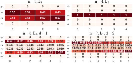
[image:2.612.311.565.186.306.2]In this paper, we focus on count queries, a fundamental problem in private data release that underpins many applica-tions, from basic statistics of a dataset to complex spatial and graphical distributions. Count queries are needed to materialize frequency distributions, instantiate statistical models, and as the basis of SQL COUNT * queries. Counts can be applied to arbitrary groups, and based on complex predicates; hence they represent a very general tool. Abstracting, we have a
Fig. 1: Heatmaps of unconstrained mechanisms forα=0.62
group ofnindividuals, who each hold a private bit (encoding,
for example, whether or not they possess a particular sensitive characteristic). The aim is to release information about the sum of the bits, while meeting the stringent differential privacy guarantee. The usual model assumes the existence of a trusted aggregator, who receives the individual bits, and who aims to release a noisy representation of their sum. Since the value of
the true answer is in{0. . .n}, it is natural to restrict the output
of the mechanism to this range also, to ensure downstream compatibility with subsequent data analysis expecting integer counts in this range. If we analyze how existing approaches to differential privacy handle this case, we find there are weak-nesses. We consider the most relevant example, mechanisms obtained via a linear programming framework.
Linear Programming Framework [3] (cf. Section III).
Ghosh et al. considered count queries and proved powerful
theorems about utility-optimal mechanisms. They showed how to design mechanisms for count queries which minimize a loss function, via linear programming. The mechanisms obtained by solving linear programs specify, for each possible input, a probability distribution over allowable outputs. However, for common objectives, including to minimize the expected
absolute error (denoted L1) and squared error (L2), we
ob-served that the “optimal” mechanisms have some anomalous behavior, such as never reporting some values.
Figure 1 gives some examples of this phenomenon in action. We show four optimal mechanisms generated by solving linear
program described in section III for different input sizes (n),
under a privacy guarantee controlled by a parameter α
(ex-plained later, and set to a fixed value here). Each column gives
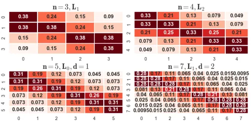
Fig. 2: Heatmaps of constrained mechanisms forα=0.62
for a given input count (also 0 ton). The case of optimizing the
squared error (L2) is most striking: the “optimal” thing to do in
this case is to ignore the input and always report ‘2’! But other cases are also problematic: all these optimal mechanisms never report some outputs (gaps), and disproportionately report some others (spikes). For example, minimizing the absolute error for
n=7 has a chance of reporting the values 2 or 5 with at least
0.7 probability, regardless of the input value. Similarly, if we
try to minimize the probability of reporting an answer that is
more than 1 step away from the true input (denoted asL0with
d=1), there is an over 90% chance of reporting 1 or 4.
Clearly, such results are counter-intuitive and show that blind optimization of simple objective functions leads to unexpected and undesirable outcomes. To address this, we
initiate the study of constrained mechanism design: requiring
mechanisms to satisfy additional properties ensuring desired structure in obtained mechanism and avoiding these
patholo-gies. For example, we define the notion of fairness, which
requires that the probability of reporting the true input is the
same for all inputs; and weak honesty, where we require that
the probability of reporting the true input is at least uniform
(i.e. at least n+11). These both ultimatel entail that every output
is reported with a non-zero probability. We also consider various monotonicity properties, which preclude big spikes in probability for responses that are far from the truth. In total, we describe seven natural properties that one could demand of a mechanism. Our first result is to show how to extend the linear programming framework to incorporate these properties and eliminate pathological outcomes.
Figure 2 shows the heatmap of constrained mechanisms satisfying all properties. The anomalies (spikes and gaps) seen in Figure 1 are now eliminated. Recall that optimizing
in the unconstrained L2 case returns a trivial solution that
outputs 2 irrespective of input. Now, the probability mass in the corresponding constrained mechanism is more distributed
and with probability at least 23, the mechanism outputs a value
differing from the true answer by at most 1 for all inputs. Similar observations can be made in the other instances. We go on to perform a detailed study of constrained mechanism design for count queries, and show some surprising outcomes: • No blow up in number of mechanisms for L0. Given 7
different properties, there are 27=128 different combinations
that could be requested. Does this mean that there are over a
hundred distinct constrained mechanisms? We show that this is not the case: there are at most four different behaviours that can be observed. Two behaviors correspond to explicit constructions of mechanisms: the (truncated) geometric
mech-anism (GM) proposed in [3], which corresponds to the
uncon-strained optimal solution; and a new “explicit fair mechanism”
(EM) which simultaneously achieves all the properties that
we introduce. In between are two mechanisms which achieve variations of the weak honesty property above, which are found by solving an optimization problem.
• No significant loss in utility. The Geometric mechanism
obtains the minimal value of theL0 loss function, for which
we give a closed form in terms of the privacy parameter α.
However, our most constrained mechanism (the explicit fair
mechanism, EM) is only incrementally more expensive: the
loss function value is higher by a factor of approximately 1+
1
n, which becomes negligible for even moderaten. The costs of
the other constrained mechanisms are sandwiched in between.
Consequently, we conclude that the addition of constraints provides significant structure to the space of mechanism de-sign, and comes at very low cost. Given these observations, one may wonder whether there is any material difference in behavior between the constrained and unconstrained mecha-nisms? This is indeed the case. For example, Figure 7 shows a
quantitative difference betweenGMandEMforn=4 (chosen
to make the results easy to view). The heatmap shows thatGM
concentrates the probability mass on the two extreme outputs,
0 and n, while EM achieves a more balanced distribution,
closer to the leading diagonal (corresponding to a truthful
mechanism). If we assume a uniform input distribution, EM
reports the true input with probability 0.224, whileGM(which
maximizes this quantity) achieves 0.238, only marginally higher but with a high skew. A third mechanism with the weak
honesty property,WM, sits between the two.
Our experiments further study the implications of using constrained mechanisms, and compare their empirical behavior on a mixture of real and synthetic data. Differences are most
apparent for moderate values of n: as n becomes very large,
these “end effects” become less significant, and off-the-shelf mechanisms do a good enough job. Thus, we spend most of our effort studying groups corresponding to a moderate number of individuals, up to tens. Arguably, such small groups are most in need of protection, since they have only a few participants: there is reduced safety in numbers for them.
II. PRELIMINARIES
A. Model And Definitions
Our model captures a group ofnparticipants, each of whom
has some private information which is encoded as a single bit. They share their information with a trusted aggregator, whose aim is to release information about the sum of the values while protecting the privacy of each participant. Although simple, this question is at the heart of all complex analysis and modelling, and demands a comprehensive solution. We simplify the description of the input to just record the true
sum of values j, so we have 0≤ j≤n. This captures the
case of a count-query over a tableD. Our goal is to design a
randomized mechanism that, given input j produces outputi, subject to certain constraints.
Definition 1 (Randomized Mechanism): A randomized
me-chanism Mis a mappingM:D⇒R, whereR={0, ..,n}=
[n] is the range of the mechanism. We write PrM[i|j] for the
conditional probability that the output M(j)(on input j∈D)
is i∈R. We will drop the subscriptM in context.
Our mechanism maps inputs in the range 0 to nto outputs
in the same range. While one could allow a different set of outputs, it is most natural to restrict to this range. Consider for example, a downstream analysis step which expects counts
to be integers in the range [n]: we should ensure that this
expectation is met by the result of applying mechanisms. Rather than attempt to map different outputs to this range, it is more direct to build mechanisms that cover this output set. It is
therefore natural to representMas an(n+1)×(n+1)square
matrix P, where Pi,j=Pr[M(j) =i] =PrM[i|j]. For brevity,
we abbreviate this probability to Pr[i|j]. Note that thereforeP
is acolumn stochastic matrix: the entries in each column can be interpreted as probabilities, and sum to 1.
Privacy of a mechanism. Differential privacy imposes con-straints on the probabilities in our mechanism. Specifically, it bounds the ratio of probabilities of seeing the same output for neighboring inputs [1]. In our setting, the notion of neighboring is simply that they differ by (at most) one, which happens when an individual changes their response. Hence, applying the definition, we obtain
Definition 2 (Differentially Private Mechanisms):
MechanismM isα-differentially private for α∈[0,1]if
∀i,j:α≤PrPr[i[|ij|+j]1]≤α1.
Here α close to 1 provides a stronger notion of privacy and
a tighter constraint on the probabilities, while α close to zero
relaxes these constraints. It is common in differential privacy
to writeα=exp(−ε)≈1−ε, for some ε>0. We adopt the
α notation for conciseness, and translate results in terms ofε
-differential privacy when appropriate. We say a DP constraint is tightif the relevant inequality is met with equality.
Utility of a mechanism. The true test of the utility of a mechanism is the accuracy with which it allows queries to be answered over real data. However, we aim to design mechanisms prior to their application to data, and so we seek a suitable function to evaluate their quality. Since there are
many column stochastic matrices that satisfy DP, the problem of finding a mechanism that provides the maximal utility can be framed as an optimization problem. Specifically, we can encode our notion of utility as a penalty function, where we seek to penalize the mechanism for reporting results that are far from the true answer.
Definition 3 (Objective function value): We define the
ob-jective functionOp,⊕(P)of a mechanismP as:
Op,⊕(P) =⊕j
∑
iwjPr[i|j]|i−j|p
where⊕is an operator like∑or max, and ∑jwj=1.
Observe that the weights wj can be thought of as a prior
distribution on the input values j. Then Op,∑(P) gives the
expected error of the mechanism, when taking its output as
the true answer, and |i−j|p penalizes the extent by which
the output was incorrect. When not otherwise stated, we take
wj = n+11, i.e. a uniform prior over the inputs. Common
choices for pin the definition would be p=2, corresponding
to a squared error (L2 norm), p=1, corresponding to an
absolute error (L1 norm), and p=0, corresponding to the
probability of any wrong answer (L0norm). In what follows,
we devote most of our attention to the case L0. We argue
that this is an important case: (i) maximizing the probability of reporting the truth is a natural objective in mechanism design; we aim to ensure that the reported answer is the maximum likelihood estimator (MLE) for the true answer, for use in downstream processing (ii) due to the differential privacy constraints, maximizing the probability of the true answer has the additional effect of making nearby answers likely, as our experiments validate. (iii) our internal study
shows that objectives likeL1 and L2 often give pathological
results, as seen in Figure 1. Working with L0 gives more
robust behavior. We therefore initiate the study of constrained
mechanism design for L0, and give some initial results for
other objectives. It is convenient to apply a rescaling of the
loss function by a factor of n+n1: this sets the cost of a trivial
mechanism to 1 (Definition 5). We refer to this rescaled cost
as L0, as this corresponds to a scaled version of O0,∑ that
sums the probabilities of a wrong answer, and so
L0(P) =
n+1
n −
traceP
n . (1)
Abusing notation slightly, we also define the objective function, L0,d = n+n1∑ni,j:|i−j|≥dwjPr[i|j] which computes a
rescaled sum of probabilities more than d steps off the main
diagonal, so that L0=L0,0.
B. Prior Work and Existing Mechanisms
The most relevant work to our interests is due to Ghoshet
al. [3] who study the problem of designing mechanisms
opti-mizing for expected utility. Their contributions are to introduce a linear programming formulation of the problem, and to show
that a certain mechanism (denoted GM) emerges as the basis
of other optimal mechanisms, discussed in more detail below. Gupte and Sunararajan proved a similar universality result for
“minimax” loss functions and uniform weightswj [11]. They
provided a simple test for when a given mechanism can be
obtained by first applying GM and then modifying the result
(e.g. by randomly sampling from a distribution indexed by
the observed output from GM). Subsequent work by Brenner
and Nissim shows that such “universally optimal” mechanisms are not possible in general for other computations, such as computing histograms [12]. Other relevant work studies special cases of differential privacy. An important variant is
the model of local differential privacy (LDP), where users
first perturb their input before passing it to an (untrusted) aggregator. That is, each user applies a mechanism for a
group of size n=1. LDP is used in Google’s Chrome via the
RAPPOR tool to collect browser and system statistics [13], and in Apple’s iOS 10 to collect app usage statistics [14]. The most relevant existing approaches to us are the following:
Mechanisms from coin-tossing: Randomized Response.
There are many variations of Randomized Response [15]. A
canonical form for the casen=1 has the user report the true
value of their input bit with probability p>12, but report the
negation of their input with probability 1−p. It is immediate
that this procedure achievesα-differential privacy forα=1−pp
(see Definition 2). Due to its simplicity and privacy guarantees, randomized response has recently found use in a number of systems, such as RAPPOR [13], which applies randomized response in conjunction with a Bloom filter to accommodate
many possible elements. Geng et al. in [16] give a natural
extension of 1 bit randomized response to n-ary data, which
reports its input with probability p, else another output is
chosen uniformly. This gives low utility for count queries.
Defining sampling probabilities: Exponential Mechanism.
McSherry and Talwar [17] proposed the Exponential
Mecha-nism as a generic approach to designing mechaMecha-nisms. Let D
be the domain of input dataset and Rthe range of perturbed
responses. The crux of the exponential mechanism is in
designing a quality function Q:D × R ⇒R so that Q(d,r)
measures the desirability of providing output r for input d.
The mechanism is then defined by setting
Pr[r∈ R|d] =exp
εQ(d,r)
2s
.
∑r0∈Rexp
εQ(d,r0)
2s
(2)
where s captures the amount by which changing an
indi-vidual’s input can alter the output of Q in the worst case.
It is proved that this mechanism obtains at least exp(−ε)
-differential privacy. However, although we can use Q to
indicate that some outputs are more preferred, it is not possible
to modify a givenQto directly enforce the properties that we
desire, such as ensuring that the probability of returning the true output is at least as good as that of a uniform distribution (“weak honesty”, (13)).
Rounding numeric outputs: Laplace and Geometric Mech-anisms. Perhaps the best known differentially private mech-anism is the Laplace mechmech-anism, which operates by adding random noise to the true answer from an appropriately scaled Laplace distribution (a continuous exponential distribution symmetric around zero). Note that in order to fit our definition of a mechanism (Definition 1), it will be necessary to round
and truncate the output of the mechanism to the range [n].
Here, the Laplace mechanism does not easily fit the require-ments. Instead, the appropriate method is the discrete analog of the Laplace mechanism, which is the (truncated) Geometric
mechanism, introduced by Ghoshet al. [3], who showed that
it is the basis for unconstrained mechanisms.
Definition 4: Range Restricted Geometric Mechanism [3]
(GM) Letqbe the true (unperturbed) result of a count query.
The GM responds with min(max(0,q+δ),n), where δ is a
noise drawn from a random variable X with a double sided
geometric distribution, Pr[X=δ] =(11−+αα)|δ| for δ∈Z.
That is,GMadds noise from two sided geometric
distribu-tion to the query result and remaps all outputs less than 0 onto
0 and greater than n ton. ThoughGM does not include any
zero rows, we observe that each column distribution in GM
has spikes at the extreme values, which tend to distort the true distribution quite dramatically, as the next example shows.
Example 1: Consider the case of n=2, corresponding to a group of two individuals, with a moderate setting of the
privacy parameterα=109. For an input of 1 (i.e. one user has
a 1, and the other has a 0), we obtain that the probability of
seeing an output of 0 is ≈0.47, and the same for an output
of 2. Meanwhile, the probably of reporting the true output
is ≈0.05 — in other words, the chance of seeing the true
answer is eighteen times lower than seeing an incorrect answer. Meanwhile, if the input is 0, then output 0 is returned with
probability≈0.53: so the mechanism is much more likely to
report the true answer when it is 0 than when it is 1. As we
increase the privacy parameter α closer to 1 (more privacy),
the probability of outputs other than 0 and napproaches 0.
III. UNCONSTRAINEDMECHANISMDESIGN
A natural starting point is to use optimization tools to find optimal mechanisms. Following [3], the key observation is that the DP requirements can be written as linear constraints over variables which represent the entries of the mechanism. The objective function is also a linear function of these variables.
Formally, we define variablesρi,j for Pr[i|j], and write:
minimize:
n
∑
j=0
wj n
∑
i=0
|i−j|pρi,j (3)
subject to: 0≤ρi,j≤1 ∀i,j∈[n] (4)
n
∑
i=0
ρi,j=1 ∀j∈[n] (5)
ρi,j≥α ρi,j+1, andρi,j+1≥α ρi,j ∀i∈[n],j∈[n−1] (6)
(6) encodes the differential privacy constraints. Finally, (3) encodes a loss function of Definition 3 for the notion of utility we aim for. We refer to the set of constraints (4), (5) and (6)
as BASICDP. The result is a linear program with a quadratic
number of variables, and a quadratic number of constraints, each containing at most a linear number of variables. There-fore, solving the resulting LP obtains a mechanism minimizing the given objective function with the desired properties, in time
polynomial in n.
Applying this approach yields results like those in Figure 1. Our studies found that similar undesirable results were found
across a range of choices of n, α and loss function. Simple
attempts to prevent these outcomes are not effective. For example, we can ensure that no entry is zero by adding a constraint to the LP enforcing this. However, the consequence is that rows which were zero are now set to be the smallest allowable value, which is unsatisfying. Instead, we propose an additional set of properties to eliminate degeneracy and provide more structure in our solutions.
IV. CONSTRAINEDMECHANISMDESIGN
A. Structural Constraints
We now propose a set of structural properties that help to control the objective function in addition to meeting differen-tial privacy. We believe that these constraints are natural and intuitive and often observed in other mechanisms satisfying differential privacy. We present properties of three types: those which operate on rows of the matrix, those which apply to columns of the matrix, and those which apply to the diagonal.
Row Honesty (RH):A mechanism is row honestif
∀i,j.Pr[i|i]≥Pr[i|j] (7)
Row honesty means that a mechanism should have higher
probability of reporting i when the input is i than for any
other input.
Row Monotone (RM):A mechanism is row monotoneif
∀1≤ j≤i: Pr[i|j−1]≤Pr[i|j]
∀i≤j<n: Pr[i|j+1]≤Pr[i|j] (8)
This property generalizes row honesty: row monotonicity
implies row honesty. It requires that entries in row i are
monotone non-increasing as we move away from the diagonal
element Pr[i|i]. Note that row monotonicity is independent of
differential privacy: we can find mechanisms that achieve DP but are not row monotone, and vice-versa.
Analogous to the row-wise properties, we define monotonic-ity and honesty along columns also.
Column Honesty (CH): A mechanism is column honestif
∀i,j: Pr[j|j]≥Pr[i|j]. (9)
Column honesty requires that the mechanism be honest
enough to report the true answer more often than any
individ-ual false answer. As demonstrated by Example 1, GM does
not obey column honesty.
Column Monotone (CM): A mechanism iscolumn monotone if
∀1≤i≤ j: Pr[i−1|j]≤Pr[i|j]
∀j≤i<n: Pr[i+1|j]≤Pr[i|j] (10)
As in the row-wise case, column monotonicity implies column honesty (but not vice-versa). It captures the property that outputs closer to the true answer should be more likely than those further away.
Fairness (F): A mechanism is fair when the probability of reporting the true input is constant, i.e.
∀i,j: Pr[i|i] =Pr[j|j]:=y. (11)
Example 1 shows that GM is not a fair mechanism. If a
mechanism is fair and has row honesty, then all off-diagonal
elements are at mosty, so the mechanism also satisfies column
honesty. Symmetrically, a fair and column honest mechanism is row honest. While this may seem like a restrictive constraint, we observe that mechanisms proposed in other contexts have this property, such as the staircase mechanism of [16].
Lemma 1: If a mechanism is required to be fair, then any
mechanism that minimizes the objective O0,∑ is
simultane-ously optimal for all settings of weights wj.
Proof:Let the diagonal element of the fair mechanism be
y. The objective function value is
∑
j∈[n]i
∑
∈[n]wjPr[i|j](i−j)0=
∑
j∈[n]wj(1−y) =1−y (12)
That is, the value is independent of thewjs.
Weak Honesty (WH): A mechanism satisfiesweak honestyif
∀i: Pr[i|i]≥ 1
n+1 (13)
We can consider this property a weaker version of column
honesty, as CH implies WH: for any column j, summing the
column honesty property over all rowsi, we obtain
(n+1)Pr[i|i] =
n
∑
i=0
Pr[j|j]≥
n
∑
i=0
Pr[i|j] =1
so after rearranging, we have Pr[i|i]≥ 1
n+1.
Weak honesty ensures that a mechanism reports the true answer with probability at least that of uniform guessing
(formalized as the uniform mechanismUMin Definition 5). It
also ensures that the mechanism does not have any rows that are all zero (corresponding to outputs with no probability of
being produced).GMdoes not always obey weak honesty, as
is shown by Example 1.
The final property we consider is a natural symmetry
property (formally, it is that the matrixP iscentrosymmetric):
Symmetry (S):A mechanism is symmetric if
∀i,j: Pr[i|j] =Pr[n−i|n−j] (14)
Theorem 1: Given a mechanism M which meets a subset
of properties P from those defined above, we can construct
a symmetric mechanism M∗ which also satisfies all ofPand
achieves the same objective function value asM.
We defer this proof to the Appendix.
Consequences of these properties. We first argue that these properties all contribute to avoiding the degenerate mecha-nisms shown above. The (column, row) honesty and mono-tonicity properties work to prevent the “spikes” observed when a value far from the true input is made excessively likely. The (column) honesty properties do so by preventing a far output being more likely than the true input; the (column) monotonicity properties do so more strongly by ensuring that any further output is no more likely than one that is nearer to the true input. Fairness, column honesty and weak honesty prevent gaps (zero rows): they ensure that the diagonal entry in each row is non-zero, and then the DP requirement ensures that all other entries in the same row must also be non-zero.
A simple observation is that in the (trivial) n=1 case,
randomized response is the unique optimal α-differentially
private mechanism under any objective function Op,∑. It is
straightforward to check that the resulting mechanism meets
all the above properties when p ≥ 1
2. We next show that
there is an efficient procedure to find an optimal constrained
mechanism for any n>1.
Theorem 2: Given any subset of the structural constraints, we can find an optimal (constrained) mechanism which
re-spects these constraints in time polynomial in n.
Proof:We break the proof into two pieces. First, we argue that given any subset of structural constraints we can create a Linear Program describing it, and second we argue that there exists a mechanism satisfying them all. Observe that all seven properties listed above can be encoded as a linear constraints. For example, symmetry is written as
ρi,j=ρn−i,n−j ∀i,j∈[n]
while weak honesty is
ρi,i≥1/(n+1).
Row monotonicity becomes
ρj,i−1≤ρj,i ∀j∈[n],i<j
ρj,i+1≤ρj,i ∀i∈[n−1],j<i
Consequently, we can create a linear program of size
poly-nomial inn, by adding these to the BASICDP constraints (4),
(5) and (6) established in Section III. This shows the first part of the proof. Next, we show that any such LP is feasible by defining a trivial baseline mechanism:
Definition 5 (Uniform Mechanism, UM): The uniform me-chanismof sizen has Pr[i|j] =n+11, for alli,j∈[n].
That is,UMignores its input and picks an allowable output
uniformly at random. It demonstrates that all our properties are (simultaneously) achievable, albeit trivially. By observation,
the mechanism is symmetric and fair for any α0≤1. It meets
x xα xα2 xα3 · · · xαn yα y yα yα2 · · · yαn−1 yα2 yα y yα · · · yαn−2 yα3 yα2 yα y · · · yαn−3 yα4 yα3 yα2 yα · · · yαn−4
..
. ... ... ... . .. ...
xαn xαn−1 xαn−2 xαn−3 · · · x
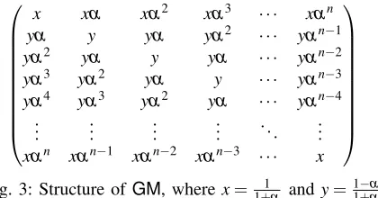
[image:7.612.336.546.52.162.2]
Fig. 3: Structure ofGM, where x=1+α1 andy=1−α
1+α
the inequalities specified for row monotonicity, column
mono-tonicity and weak honesty with equality. UM also satisfies
differential privacy for allα≤1.
Clearly,UMis undesirable from the perspective of providing
utility. We easily calculate that the objective function value
O0,∑ achieved byUMis
n
n+1, which is close to the maximum
possible value of 1. Note that we chose our definition of theL0
function to assign this mechanism a (reweighted) score of 1.
B. The Geometric Mechanism
Next, we revisit the (range restricted) Geometric
Mecha-nism,GM (Definition 4). In Figure 3, we show the structure
of the mechanism, which can be derived by simple calculation from Definition 4. Below, we show that it enjoys a number of
special properties. In prior work, Ghosh et al. showed that
GMplays an important role, as it can be transformed into an
optimal mechanism for different objectives. Here, we argue (proof omitted due to space constraints) a more direct result:
that GMis directly optimal for a uniform objective function1
Theorem 3: GM is the (unique) optimal mechanism
satis-fying BASICDP under theL0objective function.
Limitations ofGM.SinceGMis ‘optimal’ forL0, should we
conclude our study here? The answer is no, since GM fails
to satisfy many of the desirable properties we identified in Section IV-A, and as illustrated in Example 1. We have already
observed thatGM is not fair, and does not in general satisfy
column honesty (or column monotonicity) or weak honesty. Next, we identify parameter settings for when they do hold.
Lemma 2: GMobeys weak honesty iff n≥ 2α
1−α.
Proof: Weak honesty requires the diagonal elements to
all exceed n+11. Since y<x, we focus on y. We require y≥
1
n+1 i.e 1−α
1+α ≥
1
n+1. This reduces to n+1≥
1+α
1−α, giving the
requirementn≥ 2α
1−α.
GM satisfies the column monotonicity condition for many
i,j pairs. The critical place in the matrix where it can be
violated is between the first and second rows (symmetrically, between penultimate and final rows). This corresponds to the
problematic behavior ofGM to report extreme outputs (0 or
n) disproportionately often.
Lemma 3: GMachieves column monotonicity iffα≤12. Proof:We require Pr[1|1]≤Pr[0|1], i.e.y≤αxor 1−α
1+α ≤ α
1+α. This gives the conditionα ≤
1
2. It is straightforward to
check that this ensures monotonicity in all other columns.
1Note that, compared to [3], we define mechanisms to enforce differential
y yα yα2 yα3 yα4 yα4 yα4 yα4 yα y yα yα2 yα3 yα3 yα3 yα3 yα yα y yα yα2 yα3 yα3 yα3 yα2 yα2 yα y yα yα2 yα2 yα2 yα2 yα2 yα2 yα y yα yα2 yα2 yα3 yα3 yα3 yα2 yα y yα yα yα3 yα3 yα3 yα3 yα2 yα y yα yα4 yα4 yα4 yα4 yα3 yα2 yα y
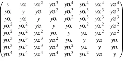
[image:8.612.71.280.52.156.2]
Fig. 4: Explicit fair mechanism forn=7
By inspection,GMis always symmetric, and row monotone.
The (L0) objective function value achieved byGMis
n+1
n 1−
(n−1)y+2x n+1
=n+n1 1−n−1
n+1 1−α
1+α−
2
(1+α)(n+1)
= 2α
1+α
We next design a different explicit mechanism which achieves more of the desired properties.
C. Explicit Fair Mechanism
Although we can achieve any desired combination of prop-erties by solving an appropriate linear program, it is natural to ask whether there is any non-trivial explicit mechanism that achieves properties such as fairness with an objective
function score comparable to that of GM. We answer this
question in the positive. First, we consider the limits of what
can be achieved under fairness. In the case of GM, all DP
inequalities are tight. This is not possible when fairness is
demanded. A fair mechanismMwith all DP inequalities tight
would be completely determined: Mi,j=yα|i−j| for some y.
It is easy to calculate for any such mechanism that there
is no setting of y which ensures that all columns sum to
1, a contradiction. Hence, we cannot have a fair mechanism with all DP inequalities tight. Nevertheless, trying to achieve tightness provides us with a bound on what can be achieved.
Lemma 4: LetFbe a fair mechanism of size(n+1)×(n+
1)withyas the diagonal element. Theny≤ 1−α
1+α−2α
n 2+1. Proof: There are some slight differences depending on
whether we consider odd or even values of n. Without loss
of generality, take n even. We will consider a fixed column
j. For all i, we are required to have Pr[i|i] =y for some y.
Repeatedly applying the DP inequality, we obtain an upper
bound involvingyas Pr[i|j]≥yαi−j when j<iand Pr[i|j]≥
yαj−i wheni>j. Summing these for any given column jand
equating to 1 provides an upper bound ony. We get the tightest
bound by picking column j=n
2. Theny+2y∑
n 2
j=1αj≤1, so:
y≤ 1
1+2∑
n 2
j=1αj
= 1−α
1+α−2αn2+1
(15)
For n large enough, we can neglect the αn/2+1 term, and
approximate this quantity by 1−α
1+α.
Note that for optimality under an objective function Op,∑,
we should make y as large as possible. Hence, any optimal
mechanism will have yas close to this value as possible.
In-deed, the above proof helps us to design an explicit mechanism
EM that achieves fairness. The proof argues that in column
n/2, the smallest values we can obtain above and below the
yentry are αy,α2yand so on up toαn/2y. Then the sum of
these terms is set to 1. All other columns must also sum to 1; a simple way to achieve this is to ensure all columns contain a permutation of the same set of terms. To ensure DP is satisfied, we should arrange these so that row-adjacent entries differ in
their power ofα by at most one.
Our explicit fair mechanismEMis then defined as follows:
Pr[i|j] =
(
yα|i−j| if|i−j|<min(j,n−j) yαd
|i−j|+min(j,n−j)
2 e otherwise
(16)
Here, y is set to 1−α
1+α−2αn/2+1, i.e. the value determined
in Equation (15). From the proof of Lemma 1 and (1), we
have that theL0 score of this mechanism is n+n1(1−y), as it
maximizesysubject to the bound of Lemma 1.
Figure 4 shows the instantiation of this mechanism for
the case n=7. Comparing to GM, we see that the diagonal
elements are slightly increased, with the exception of the two corner diagonals, which are decreased. It is tempting to try to obtain the mechanism via the Exponential Mechanism, by
using a quality function applied to |i−j| similar in form
to (16). Note however, that the constant factors of 2 in its definition (2) leads to a considerably weaker result than this explicit construction, equivalent to halving the privacy
parameter ε. It is easy to check that in the n=7 example,
the mechanism is symmetric, and meets all of the properties defined in Section IV-A. In fact, this is the case for all values
ofn. The proof is rather lengthy and proceeds by considering
a number of cases; we omit it for brevity.
Theorem 4: EM is an optimal mechanism under L0 that satisfies all properties listed in Section IV-A.
D. Comparing mechanisms
In Section IV-A, we define 7 different properties, denoted as RH, RM, CH, CM, WH, F, and S. We can seek a mechanism that satisfies any subset of these, suggesting that there are 128 combinations to explore. However, we are able to dramatically reduce this design space with the following analysis based on
theL0 score function.
First, we have shown by Theorem 4 that EM has the
optimal L0 score of any fair mechanism and has all other
possible properties “for free”. Therefore, for any desired set
of properties that include F, we can just useEM.
Second, we have shown by Theorem 3 that GM achieves
symmetry and row monotonicity (and hence row honesty) at
a cost which is optimal for any mechanism (i.e. BASICDP).
Hence for any subset of{S, RM, RH}, it suffices to useGM.
In our experiments (Section V-A), we show that there are only two remaining behaviors: either we solve the LP for the WH property alone, or we solve the LP for WH and CM properties. Both solutions come with symmetry (S) and row properties RH, RM at no additional cost. However, as noted
in Lemma 2,GMsatisfies WH whenn≥ 2α
1−α, so in this case,
Want Fairness?
Fair Mechanism
Want Column Property?
n≥ 2α 1−α?
Want Weak Honesty?
Geometric
Mechanism WH
WH + CM yes no
no
yes
yes no
no
[image:9.612.306.568.52.144.2]yes
Fig. 5: Flowchart of properties for L0objective (α>12)
Property GM WM EM UM
Symmetry (S) Y Y Y Y
Row Monotone (RM) Y Y Y Y
Column Monotone (CM) — — Y Y
Fairness (F) N N Y Y
Weak Honesty (WH) — Y Y Y
L0 12+αα ≥12+αα ≈ 12+αα ·n+n1 1
Fig. 6: Properties of named mechanisms
have that CM ⇒ CH ⇒ WH, so any demand that requires
any of these properties (and not F) can be satisfied by WM
also. But in the weak privacy case that α≤12,GMhas these
properties, and so subsumes WM.
To summarize this reasoning, in the case that α ≤ 12,
there are only two competitive mechanisms: EMif fairness is
required, andGMfor all other cases. Whenα>12, things are
a little more complicated, so we show a flowchart in Figure 5: from 128 possibilities, there are only four distinct approaches to consider (two explicit mechanisms, and two solutions to an LP with different constraints), and the choice is determined primarily by whether the mechanism is required to satisfy fairness, column properties, weak honesty, or none. We also
consider the baseline methodUMfor comparison. We present
a summary of these four named mechanisms in Figure 6: the
explicitGM,UMandEM, andWMwhich is found by solving
an LP. We write ‘—’ for a property when this depends on the setting of the parameters (discussed in the relevant section).
We see that EM has a very similar objective function value
L0 (recalling that we are trying to minimize this value), and
all the properties considered so far. We do not have a closed
form for the L0 score of WM, as it is found by solving the
LP; however it is no less than that forGM(sinceGMsatisfies
a subset of the required properties ofWM), and no more than
that of EM(sinceEM satisfies all properties).
At this point, we might ask how different are these
mech-Fig. 7: Heatmaps forGM,EM,WMwithn=4
[image:9.612.90.259.55.265.2]anisms in practice — perhaps they are all rather similar? Figure 7 shows this is not the case for a small group size
(n=4). For a moderate value of the privacy parameterα=0.9,
it presents the three non-trivial mechanisms using a heatmap to highlight where the large entries are. We immediately see that
EM concentrates probability mass along a uniform diagonal
(as required by fairness). Both GM and WM tend to favor
extreme outputs (0 or 4 in this example) whatever the input,
althoughGMis very skewed in this regard whileWMis more
uniform in allowing non-extreme outputs.
Last, we check that what we are doing is not a trivial modifi-cation of known mechanisms. Prior work [3], [11] showed how
optimal unconstrained mechanisms can be derived fromGM
by transformations. Gupte and Sundarajrajan give a simple
test: a mechanismP can be derived fromGMiff every set of
three adjacent entries in the mechanism satisfy
(Pr[i|j]−αPr[i|j−1])≥α(Pr[i|j+1]−αPr[i|j])
We applied this test to mechanismsWMand verified that this
condition is indeed violated forn>1. ForEM, this condition
is automatically broken for alln>1: we have Pr[2|0] =Pr[2|1]
=yα, while Pr[2|2] =y. Then the condition is
yα(1−α)≥yα(1−α2)≡1≥(1+α)
which is always false forα>0. Hence, these mechanisms are
not derivable from GM.
V. EXPERIMENTALSTUDY
In Section V-A, we substantiate our earlier claims about properties of mechanisms satisfying weak honesty (but not fairness). In what follows, we look at other measures of utility of these mechanisms, to understand their robustness.
Default Experimental Settings.All experiments in this work were implemented in Python, making use of the standard library NumPy to handle the linear algebraic calculations, and PyLPSolve [18] to solve the generated LPs. Evaluation was made on a commodity machine running Linux. We omit detailed timing measurements, as the time to solve the LPs generated was negligible (sub-second).
Experimental Setting. We considered a variety of settings
of parameterα (typical values chosen are{12,32,1011,10099} and
group size n(ranging from 2 up to hundreds).
A. L0 Objective Function
Our first experiment analyzes the effect of weak honesty
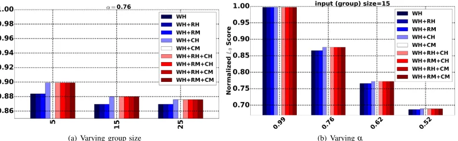
[image:9.612.50.300.297.372.2](a) Varying group size (b) Varyingα
Fig. 8: Combinations Of Properties with Weak Honesty
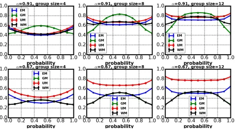
(a) α=2
[image:10.612.55.555.62.502.2]3 (b)α=1011 (c) α=10099
Fig. 9: Final Groups Of Mechanisms with Distinct Behaviors
(a) Estimating young population (b) Estimating gender balance (c) Estimating income level
Fig. 10: Empirical Error Probability on Adult Dataset forα=0.9
RM}, including the empty set. There are 9 meaningful
combi-nations of properties to ask for, which we write as{/0,RH, RM,
CH, CM, RH+CH, RH+CM, RM+CH, RM+CM} — other
combinations reduce to these, since RM implies RH, and CM implies CH.
As discussed in Section IV-D, there are cases when the
solution found by solving the LP has cost 2α
1+α and is identical
toGM: these are whenn≥ 2α
1−α and only row-wise properties
are requested, consistent with Figure 5. This is borne out in Figure 8: we see that when WH alone is requested, or in combination with only row properties (RH or RM) we get a
lowerL0value than when any column properties (CH or CM)
are requested. Figure 8(a) shows the case for different values
of n. When n> 2α
1−α, which is 6.33 in this example (where
α =0.76), the cost of WH alone is 12+αα =0.864, the cost of
GM. For large α (Figure 8(b)), the cost of all combinations
of WH are the same, and identical to the cost of EM; as α
is decreased, we see two behaviors, where the lower L0cost
is that of GM. We confirmed this behavior for a wide range
of nandα values. From now on, we useWMto refer to the
mechanism with WH, RM and CM properties.
The relationship between theL0scores for the three
mech-anisms is further clarified in Figure 9. The plots show theL0
scores of GM, WM, EM and UM for different values of α.
In Figure 9(a), α =23 so the threshold 12−αα =4. Then GM
satisfies WH for the whole range of nvalues shown, so WM
converges on GM, while EM has a higher (but decreasing)
cost. For Figure 9(b),α=10/11 so the threshold is 20. Indeed,
we see that the cost of WM converges with GM at n=20.
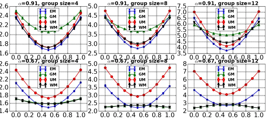
[image:10.612.53.565.241.350.2] [image:10.612.60.558.385.494.2]Fig. 11: L0,1 score for Binomial data, forn={4,8,12} andα={0.91,0.67}
Fig. 12: Histograms ofL0,d scores for Binomial data
of n values shown, so WMdoes not converge on GM here.
Rather, for this high value ofα, theyvalue forEM is above
1
n+1 for all n: so in this case EM has weak honesty, and the
cost of WMremains the same as that of the optimal fairEM.
B. Experiments On Real Data
We make use of the UCI Adult dataset, a workhorse for privacy experiments [19]. Our instance of the dataset contains demographic information on 32K adults with 15 columns listing age, job type, education, relationship status, gender, and (binary) income level. We created three binary targets, treated as sensitive: income level (high/low), gender (male/female),
and young (age over/under 30). To form small groups, we gathered the rows (corresponding to individuals) arbitrarily into groups of a desired size.
Figure 10 shows results for theL0objective, that is, where
we focus on the fraction of times the mechanism reports an incorrect answer, as a function of group size. Specifically, we count the number of groups whose noisy count for each target attribute is not equal to their true count. We expect this quan-tity to be fairly high, as it measures how often our mechanism is honest, i.e. returns the true input. Other experiments (not shown) computed the corresponding probability for returning an answer that is close to the true one, e.g. off by at most one, and showed similar patterns. The plot includes error bars from 50 repetitions of this process to show 1 standard error.
Observe first that the performance of UM is essentially
independent of the input data: the chance of it picking the
correct answer is always 1− 1
n+1 for a group of size n, and
indeed we see this behavior (up to random variation). We would hope that our optimized mechanisms can outperform
this trivial method. Perhaps surprisingly, on this dataGMdoes
appreciably worse. This highlights the limitations ofGM. In
this data, the common inputs are around the middle of the
group size (i.e. typically close ton/2). It is on these inputs that
GMdoes poorly, and only does well for inputs that are 0 orn,
which happen to be rare in this dataset (in other words, the data
distribution does not match the prior for whichGMis optimal).
The condition of weak honesty is not sufficient to improve significantly over random guessing: for this data, we see that
WMtracksUM quite closely. It is only the most constrained
mechanism that fares better on this evaluation metric for this
data:EMwhich achieves fairness gives the best probability of
Fig. 13: Root Mean Square Error plots For Binomial data
with higher values ofα in the range 0.9 to 0.99, corresponding
to the strongest privacy guarantees adopted in prior work on differential privacy, there is not much to choose between
EM and WM, and it gets even harder to show substantial
improvement over uniform guessing. In order to understand the behaviors of the mechanisms further, we next consider synthetic data, where we can directly control the data skewness within groups.
C. Experiments On Synthetic Data
In our experiments with synthetic data we generate a
population of 10,000 individuals with a private bit and divide
them into small groups of the same size, n. Each individual
has the same probability p of having their bit be one, so
the distribution within each group is Binomial. Hence, the
expected count for each group is pn. Our experiments vary
the parameters p,n andα.
L0,1Error.Our experiments so far have uesd the target
objec-tive functionL0to evaluate the quality of the mechanism. This
is sufficient to distinguish the different mechanisms, but all mechanisms achieve a score which can be close to 1, obtained by uniform guessing. To better demonstrate the usefulness of the obtained mechanisms, we use other functions to evaluate
their accuracy. Figure 11 uses the related measure ofL0,1i.e.
the fraction of groups which output a value differing from their true answer by more than 1, as we vary data distribution
(determined byp), group sizen, and privacy parameterα. We
stress that though we use L0,1 for evaluation, we continue
to use mechanisms designed for minimizing the L0 error.
Each subplot in the figure represents a configuration ofhα,ni,
describing how L0,1 error changes with input distribution
parameter p. Each experiment is repeated 30 times and we
observe that the results have very small variance.
It is apparent that the shape of the input distribution has a pronounced effect on the quality of the output. We confirm
that GMcan do well when the input is very biased (p close
to 0 or 1), which generates more instances with extreme input values. However, when the input is more spread across the input space, the more constrained mechanisms consistently
give better results. For higherα, the constrained methods have
similar behavior, and improve only slightly over UM (while
GMis often worse than uniform). Enforcing fairness tends to
makeEMless sensitive to the input distribution, except when
the input is an extreme value (0 orn). Whenαis lower (second
row), the overall scale of error decreases and WM andGM
converge, as noted previously.
L0,d Error. In the previous experiment, we fixed d=1 and
evaluated our mechanisms for variety of input distributions.
Next we varydwhile holding input size and input distributions
and compute L0,d error. Figure 12 plots the fraction of
population reporting a value that is more than d steps away
from the true answer for various d values with n=8. This
captures the probability mass in the tail of each mechanism.
In the top row, we use a more proportionate input
distribu-tion. Here,EM outperforms all other mechanisms, sometimes
by a substantial fraction. Interestingly, the margin betweenEM
andGMonly increases with largerd. Once again we see that
for higherα values, use ofGMcan yield accuracy worse than
mere random guessing. For lowerα’sGM’s accuracy increases
dramatically but still remains worse thanEM’s.
In the bottom row, the input distribution is more skewed,
which tends to favorGM. However,EMdoes not do
substan-tially worse thanGM even for this biased input distribution.
The intermediate mechanism found by WM tends to fall
betweenGMandEM. We observed similar behavior for other
values of n.
overall spread of error. Figure 13 shows plots with error bars showing one standard deviation from 30 repetitions.
As seen in previous experiments, a more symmetric input
distribution (p closer to 0.5) tends to be easier for most
mechanisms — although we see cases where GM finds this
more difficult. Increasing the group size increases the RMSE, as there is a wider range of possible outputs, and the con-straints ensure that there is some probability of producing each
possible. Yet again, we see that increasing α tends to make
GMless competitive and find many cases whereGMis worse
than random guessing (UM). The interesting case may be for
fairly high privacy requirements (α=0.91), where we observe
that EM tends to give lower error across all group sizes and
input distributions.
VI. CONCLUDINGREMARKS
We have proposed and studied several structural properties for privacy preserving mechanisms for count queries. We show how any combination of desired properties can be provided
optimally underL0by one of a few distinct mechanisms. Our
experiments show that the “optimal” GM often displays the
undesirable property of tending to output extreme values (0
or n). In practice, this means it is often not the mechanism of
choice, particuarly whenα is large (above 0.7), but can be
ac-ceptable for smaller privacy parameters.EMandWMare quite
different in structure, but are often similar in performance. It is natural to consider other possible properties—for exam-ple, one could imagine taking a version of the DP constraint applied to columns of the mechanism (in addition to the rows): this would enforce that the ratio of probabilities between
neighboringoutputsis bounded, as well as that of neighboring
inputs. The next logical direction is to provide a deeper study
of mechanisms with various properties using L1 or L2 as
objective function. It will be interesting to study tailor-made linear programming mechanisms that aim to optimize other queries such as range queries.
ACKNOWLEDGMENTS
This work is supported in part by The Alan Turing Institute under the EPSRC grant EP/N510129/1, Marie Curie Career Integration Grant 618202, an AT&T Labs VURI award, and a Warwick Collaborative Postgraduate Research Scholarship.
REFERENCES
[1] C. Dwork, “Differential privacy,” inICALP, 2006. [Online]. Available: http://dx.doi.org/10.1007/11787006_1
[2] C. Dwork and A. Roth, “The algorithmic foundations of differential privacy,” Foundations and Trends in Theoretical Computer Science, vol. 9, no. 3-4, pp. 211–407, 2014. [Online]. Available: http: //dx.doi.org/10.1561/0400000042
[3] A. Ghosh, T. Roughgarden, and M. Sundararajan, “Universally utility-maximizing privacy mechanisms,” inSTOC, 2009. [Online]. Available: http://doi.acm.org/10.1145/1536414.1536464
[4] C. Dwork, F. McSherry, K. Nissim, and A. D. Smith, “Calibrating noise to sensitivity in private data analysis,” inTheory of Cryptography, Third Theory of Cryptography Conference, TCC 2006, New York, NY, USA, March 4-7, 2006, Proceedings, 2006.
[5] C. Dwork and K. Nissim, “Privacy-preserving datamining on vertically partitioned databases,” inAnnual International Cryptology Conference. Springer, 2004.
[6] E. Shi, H. Chan, E. Rieffel, R. Chow, and D. Song, “Privacy-preserving aggregation of time-series data,” inNDSS, 2011.
[7] A. D. Sarwate and K. Chaudhuri, “Signal processing and machine learn-ing with differential privacy: Algorithms and challenges for continuous data,”IEEE signal processing magazine, vol. 30, no. 5, pp. 86–94, 2013. [8] Y. Yang, Z. Zhang, G. Miklau, M. Winslett, and X. Xiao, “Differential
privacy in data publication and analysis,” inSIGMOD, 2012. [9] C. Dwork, “The promise of differential privacy. a tutorial on
algorithmic techniques.” in FOCS, 2011. [Online]. Available: http: //research.microsoft.com/apps/pubs/default.aspx?id=155617
[10] A. Machanavajjhala, X. He, and M. Hay, “Differential privacy in the wild (tutorial),” in VLDB, 2016. [Online]. Available: http: //vldb2016.persistent.com/differential_privacy_in_the_wild.php [11] M. Gupte and M. Sundararajan, “Universally optimal privacy
mechanisms for minimax agents,” in PODS, 2010, pp. 135–146. [Online]. Available: http://doi.acm.org/10.1145/1807085.1807105 [12] H. Brenner and K. Nissim, “Impossibility of differentially private
universally optimal mechanisms,” in51th Annual IEEE Symposium on Foundations of Computer Science, FOCS 2010, October 23-26, 2010, Las Vegas, Nevada, USA, 2010, pp. 71–80.
[13] U. Erlingsson, V. Pihur, and A. Korolova, “Rappor: Randomized aggregatable privacy-preserving ordinal response,” inACM CCS, 2014. [Online]. Available: http://doi.acm.org/10.1145/2660267.2660348 [14] C. Zibreg, www.idownloadblog.com/2016/06/25/
differential-privacy-overview/, 2016.
[15] A. Chaudhuri and R. Mukerjee, Randomized response: Theory and techniques. Marcel Dekker, 1988.
[16] Q. Geng, P. Kairouz, S. Oh, and P. Viswanath, “The staircase mechanism in differential privacy,” IEEE Journal of Selected Topics in Signal Processing, vol. 9, no. 7, pp. 1176–1184, Oct 2015.
[17] K. T. Frank McSherry, “Mechanism design via differential privacy,” inFOCS, 2007. [Online]. Available: https://www.microsoft.com/en-us/ research/publication/mechanism-design-via-differential-privacy/ [18] “Pylpsolve- an object oriented wrapper for the lpsolve,” www.stat.
washington.edu/~hoytak/code/pylpsolve/, 2010.
[19] C. Blake and C. Merz, “UCI machine learning repository,” 1998. [Online]. Available: https://archive.ics.uci.edu/ml/datasets/Adult
APPENDIX
Proof of Theorem 1: Our construction to achieve
sym-metry is simple. Define a matrix MS from M as (MS)
i,j=
Mn−i,n−j. Then set M∗=12(M+MS). We first observe that
M∗ is indeed symmetric, since it is equal to
1
2(Mi,j+Mn−i,n−j) = 1
2(Mn−i,n−j+Mn−(n−i),n−(n−j)) =Mn∗−i,n−j
as required by (14). The (L0) objective function value is
unchanged since (invoking (1))
trace(M∗) =12(trace(M) +trace(MS)) =trace(M)
For the other diagonal properties (fairness and weak honesty), it is immediate that if either of these properties are satisfied by
M, then they are also satisfied byM∗. We prove the claim for
row properties; the case for column properties is symmetric.
(i) Differential privacy: if we have α ≤Mi,j/Mi,j+1≤1/α
for alli,j, then this also holds forMiS,j/MiS,j+1. Summing both
inequalities, and using that min(ab,dc)≤a+c
b+d≤max( a b,
c d), this
holds forM∗, henceM∗satisfies differential privacy.
(ii) Row monotonicity: consider a pair i,j with 1≤i≤ j.
Then we haveMj,i−1≤Mj,i(from (8)). It is also the case that
n−j≤n−i<n, which means that Mn−j,n−i+1≤Mn−j,n−i
(also from (8)). Then MSj,i−1≤MSj,i. Combining these two
inequalities, we have thatM∗j,i−1≤M∗j,i.
(iii) Row honesty: if∀i,j.Mi,i≥Mi,j, thenMiS,i≥MiS,j also.