Algebraic renormalisation of regularity structures
Y. Bruned1 · M. Hairer1 · L. Zambotti2
Received: 27 October 2016 / Accepted: 17 November 2018 / Published online: 13 December 2018
© The Author(s) 2018
Abstract We give a systematic description of a canonical renormalisation procedure of stochastic PDEs containing nonlinearities involving generalised functions. This theory is based on the construction of a new class of regularity structures which comes with an explicit and elegant description of a subgroup of their group of automorphisms. This subgroup is sufficiently large to be able to implement a version of the BPHZ renormalisation prescription in this con-text. This is in stark contrast to previous works where one considered regularity structures with a much smaller group of automorphisms, which lead to a much more indirect and convoluted construction of a renormalisation group acting on the corresponding space of admissible models by continuous transforma-tions. Our construction is based on bialgebras of decorated coloured forests in cointeraction. More precisely, we have two Hopf algebras in cointeraction, coacting jointly on a vector space which represents the generalised functions of the theory. Two twisted antipodes play a fundamental role in the
construc-B
L. Zambotti[email protected] Y. Bruned
[email protected] M. Hairer
1 Imperial College London, London, UK
2 Laboratoire de Probabilités Statistique et Modélisation, Sorbonne Université, CNRS,
tion and provide a variant of the algebraic Birkhoff factorisation that arises naturally in perturbative quantum field theory.
Mathematics Subject Classification 16T05·82C28·60H15
Contents
1 Introduction . . . 1040
1.1 A general renormalisation scheme for SPDEs . . . 1046
1.2 Overview of results . . . 1049
2 Rooted forests and bigraded spaces . . . 1052
2.1 Rooted trees and forests. . . 1052
2.2 Coloured and decorated forests . . . 1054
2.3 Bigraded spaces and triangular maps . . . 1056
3 Bialgebras, Hopf algebras and comodules of decorated forests . . . 1059
3.1 Incidence coalgebras of forests . . . 1060
3.2 Operators on decorated forests . . . 1062
3.3 Coassociativity . . . 1068
3.4 Bialgebra structure . . . 1072
3.5 Contraction of coloured subforests and Hopf algebra structure . . . 1073
3.6 Characters group . . . 1082
3.7 Comodule bialgebras . . . 1083
3.8 Skew products and group actions . . . 1088
4 A specific setting suitable for renormalisation. . . 1090
4.1 Joining roots. . . 1093
4.2 Algebraic renormalisation. . . 1097
4.3 Recursive formulae . . . 1100
5 Rules and associated regularity structures . . . 1104
5.1 Trees generated by rules. . . 1106
5.2 Subcriticality . . . 1110
5.3 Completeness . . . 1112
5.4 Three prototypical examples . . . 1116
5.5 Regularity structures determined by rules. . . 1118
6 Renormalisation of models . . . 1125
6.1 Twisted antipodes . . . 1126
6.2 Models. . . 1129
6.3 Renormalised Models . . . 1132
6.4 The reduced regularity structure . . . 1139
6.4.1 An example . . . 1143
6.4.2 Construction of extended models. . . 1145
6.4.3 Renormalisation group of the reduced structure . . . 1149
Appendix A: Spaces and canonical basis vectors . . . 1151
Appendix B: Symbolic index . . . 1151
References. . . 1153 1 Introduction
RAhas a number of interesting algebraic properties. WritingT=T(RA)for the tensor algebra onRA, which we identify with the space spanned by all finite words{(a1. . .an)}n≥0 with letters in A, we define the family of functionals Xs,t onTinductively by
Xs,t()
def
=1, Xs,t(a1. . .an)
def =
t
s X
s,u(a1. . .an−1)x˙an(u)du
where 0≤s ≤t. Chen showed that this family yields for fixeds,ta character onTendowed with theshuffle product, namely
Xs,t(vw)=Xs,t(v)Xs,t(w), (1.1)
which furthermore satisfies theflow relation
(Xs,r⊗Xr,t)τ =Xs,tτ, s ≤r ≤t,
where:T→ T⊗Tis thedeconcatenation coproduct
(a1. . .an)= n
k=0
(a1. . .ak)⊗(ak+1. . .an) .
In other words, we have a function(s,t)→Xs,t ∈ T∗which takes values in the characters on the algebra(T,)and satisfies theChen relation
Xs,rXr,t =Xs,t, s ≤r ≤t, (1.2)
whereis the product dual to. Note thatT, endowed with the shuffle product and the deconcatenation coproduct, is a Hopf algebra.
These two remarkable properties do not depend explicitly on the differen-tiability of the path(xt)t≥0. They can therefore serve as an important tool if
one wants to consider non-smooth paths and still build a consistent calculus. This intuition was at the heart of Terry Lyons’ definition [46] of ageometric rough path as a function(s,t) → Xs,t ∈ T∗ satisfying the two algebraic properties above and with a controlled modulus of continuity, for instance of Hölder type
|Xs,t(a1. . .an)| ≤C|t−s|nγ, (1.3)
with some fixed γ > 0 (although the original definition involved rather a
that this setting would allow to build a robust theory of integration and of asso-ciated differential equations. For instance, in the case of stochastic differential equations of Stratonovich type
d Xt =σ(Xt)◦d Wt ,
with W : R+ → Rd a d-dimensional Brownian motion and σ : Rd → Rd⊗Rdsmooth, one can build rough pathsXandWoverX, respectivelyW, such that the mapW →Xiscontinuous, while in general the mapW → X
is simply measurable.
The Itô stochastic integration was included in Lyons’ theory although it can not be described in terms of geometric rough paths. A few years later Gubinelli [29] introduced the concept of abranched rough pathas a function
(s,t) → Xs,t ∈ H∗ taking values in the characters of an algebra (H,·)of rooted forests, satisfying the analogue of the Chen relation (1.2) with respect to the Grossman-Larsson-product, dual of theConnes-Kreimer coproduct, and with a regularity condition
|Xs,t(τ)| ≤C|t−s||τ|γ (1.4)
where |τ| counts the number of nodes in the forest τ and γ > 0 is fixed. Again, this framework allows for a robust theory of integration and differential equations driven by branched rough paths. Moreover H, endowed with the forest product and Connes-Kreimer coproduct, turns out to be a Hopf algebra. The theory ofregularity structures[32], due to the second named author of this paper, arose from the desire to apply the above ideas to (stochastic) partial differential equations (SPDEs) involving non-linearities of (random) space– time distributions. Prominent examples are the KPZ equation [23,27,31], the 4 stochastic quantization equation [1,7,21,32,43,45], the continuous parabolic Anderson model [26,36,37], and the stochastic Navier–Stokes equa-tions [20,53].
One apparent obstacle to the application of the rough paths framework to such SPDEs is that one would like to allow for the analogue of the map
s → Xs,tτ to be a space–time distribution for someτ ∈ H. However, the algebraic relations discussed above involveproductsof such quantities, which are in general ill-defined. One of the main ideas of [32] was to replace the Hopf-algebra structure with a comodule structure: instead of a single space
H, we have two spaces(T,T+)and a coaction+:T→T⊗T+such that
However, the comodule structure allows to define the analogue of a rough path as apair: consider a distribution-valued continuous function
Rd y→y ∈T∗⊗D(Rd) , as well as a continuous function
Rd ×Rd (x,y)→γx y∈ T+∗. The analogue of the Chen relation (1.2) is then given by
γx y γyz =γx z , y γyz =z, (1.5)
where the first-product is the convolution product onT+∗, while the second -product is given by the dual of the coaction+. This structure guarantees that all relevant expressions will be linear in they, so we never need to multiply distributions. To compare this expression to (1.2), think of(yτ)(·)∈ D(Rd) for τ ∈ Tas being the analogue of z → Xz,y(τ). Note that the algebraic conditions (1.5) are not enough to provide a useful object: analytic conditions analogous to (1.4) play an essential role in the analytical aspects of the theory. Once amodelX=(, γ )has been constructed, it plays a role analogous to that of a rough path and allows to construct a robust solution theory for a class of rough (partial) differential equations.
In various specific situations, the theory yields a canonical lift of any smoothened realisation of the driving noise for the stochastic PDE under con-sideration to a model Xε. Another major difference with what one sees in the rough paths setting is the following phenomenon: if we remove the reg-ularisation asε → 0, neither the canonical modelXεnor the solution to the regularised equation converge in general to a limit. This is a structural problem which reflects again the fact that some products are intrinsically ill-defined.
This is whererenormalisationenters the game. It was already recognised in [32] that one should find a groupRof transformations on the space of models and elementsMεinRin such a way that, when applyingMεto the canonical liftXε, the resulting sequence of models converges to a limit. Then the theory essentially provides ablack box, allowing to build maximal solutions for the stochastic PDE in question.
not rely on any general theory, they had to be performed separately for each new class of stochastic PDEs.
The main aim of the present article is to define an algebraic framework allowing to build regularity structures which, on the one hand, extend the ones built in [32] and, on the other hand, admit sufficiently many automorphisms (in the sense of [32, Def. 2.28]) to cover the renormalisation procedures of all subcritical stochastic PDEs that have been studied to date.
Moreover our construction is not restricted to the Gaussian setting and applies to any choice of the driving noise with minimal integrability con-ditions. In particular this allows to recover all the renormalisation procedures used so far in applications of the theory [32,38–40,42,51]. It reaches however far beyond this and shows that the BPHZ renormalisation procedure belongs to the renormalisation group of the regularity structure associated toanyclass of subcritical semilinear stochastic PDEs. In particular, this is the case for the generalised KPZ equation which is the most natural stochastic evolution on loop space and is (formally!) given in local coordinates by
∂tuα =∂x2uα+βγα (u)∂xuβ∂xuγ +σiα(u) ξi , (1.6)
where theξi are independent space–time white noises,αβγ are the Christoffel symbols of the underlying manifold, and the σi are a collection of vector fields with the property thati L2σi =, where Lσ is the Lie derivative in the direction ofσ andis the Laplace-Beltrami operator. Another example is given by the stochastic sine-Gordon equation [41] close to the Kosterlitz-Thouless transition. In both of these examples, the relevant group describing the renormalisation procedures is of very large dimension (about 100 in the first example and arbitrarily large in the second one), so that the verification “by hand” that it does indeed belong to the “renormalisation group” as done for example in [32,39], would be impractical.
In order to describe the renormalisation procedure of SPDEs we introduce a new construction of an associated regularity structure, that will be called
extendedsince it contains a new parameter which was not present in [32], the
extended decoration. As above, this yields spaces(Tex,T+ex), such thatT+ex is a Hopf algebra and Tex a right comodule over T+ex. The renormalisation procedure of distributions coded by Tex is then described by another Hopf algebra T−ex and coactions −ex : Tex → T−ex⊗ Tex and −ex : T+ex →
Tex
− ⊗ T+ex turning both Tex and T+ex into left comodules over T−ex. This construction is, crucially, compatible with the comodule structure ofTexover
Tex
+ in the sense that−exand+exare incointeractionin the terminology of
[25], see formulae (3.48)–(5.26) and Remark3.28below. Once this structure is obtained, we can definerenormalised modelsas follows: given a functional
γg
zz¯ =(g⊗γzz¯)−ex,
g
z =(g⊗z)−ex.
The cointeraction property then guarantees thatXg satisfies again the gen-eralised Chen relation (1.5). Furthermore, the action of T−exon TexandT+ex is such that, crucially, the associated analytical conditions automatically hold as well.
All the coproducts and coactions mentioned above are a priori different operators, but we describe them in a unified framework as special cases of a contraction/extraction operation of subforests, as arising in the BPHZ renor-malisation procedure/forest formula [3,24,35,52]. It is interesting to remark that the structure described in this article is an extension of that previously described in [8,14,15] in the context of the analysis of B-series for numerical ODE solvers, which is itself an extension of the Connes-Kreimer Hopf algebra of rooted trees [16,18] arising in the abovementioned forest formula in per-turbative QFT. It is also closely related to incidence Hopf algebras associated to families of posets [49,50].
There are however a number of substantial differences with respect to the existing literature. First we propose a new approach based on coloured forests; for instance we shall consider operations like
−→ ⊗ −→ ⊗
of colouring, extraction and contraction of subforests. Further, the abovemen-tioned articles deal withtwospaces in cointeraction, analogous to our Hopf algebras T−ex and T+ex, while our third space Tex is the crucial ingredient which allows for distributions in the analytical part of the theory. Indeed, one of the main novelties of regularity structures is that they allow to study random distributional objects in a pathwise sense rather than through Feynman path integrals/correlation functions and the space Tex encodes the fundamental bricks of this construction. Another important difference is that the structure described here does not consist of simple trees/forests, but they are decorated with multiindices on both their edges and their vertices. These decorations are
not inertbut transform in a non-trivial way under our coproducts, interacting with other operations like the contraction of sub-forests and the computation of suitable gradings.
In this article, Taylor sums play a very important role, just as in the BPHZ renormalisation procedure, and they appear in the coactions of bothT−ex(the
previously shown to arise naturally in the context of perturbative quantum field theory, see for example [16,18,19,22,30,44].
In general, the context for a twisted antipode/Birkhoff factorisation is that of a group Gacting on some vector space A which comes with a valuation. Given an element of A, one then wants to renormalise it by acting on it with a suitable element ofGin such a way that its valuation vanishes. In the context of dimensional regularisation, elements of Aassign to each Feynman diagram a Laurent series in a regularisation parameter ε, and the valuation extracts the pole part of this series. In our case, the space A consists of stationary random linear maps: Tex → C∞ and we havetwoactions on it, by the group of charactersG±exofT±ex, corresponding to two different valuations. The
renormalisation groupG−exis associated to the valuation that extracts the value ofE(τ)(0)for every homogeneous elementτ ∈ Texof negative degree. The
structure groupG+exon the other hand is associated to the valuations that extract the values(τ)(x)for all homogeneous elementsτ ∈ Texof positive degree. We show in particular that the twisted antipode related to the action of G+ex is intimately related to the algebraic properties of Taylor remainders. Also in this respect, regularity structures provide a far-reaching generalisation of rough paths, expanding Massimiliano Gubinelli’s investigation of the algebraic and analytic properties of increments of functions of a real variable achieved in the theory ofcontrolled rough paths[28].
1.1 A general renormalisation scheme for SPDEs
Regularity Structures (RS) have been introduced [32] in order to solve singular SPDEs of the form
∂tu =u+F(u,∇u, ξ)
whereu=u(t,x)witht ≥0 andx ∈Rd,ξis a random space–time Schwartz distribution (typically stationary and approximately scaling-invariant at small scales) driving the equation and the non-linear term F(u,∇u, ξ) contains some products of distributions which are not well-defined by classical analytic methods. We write this equation in the customary mild formulation
u =G∗(F(u,∇u, ξ)) (1.7)
whereGis the heat kernel and we suppose for simplicity thatu(0,·)=0. If we regularise the noise ξ by means of a family of smooth mollifiers
(ε)ε>0, settingξε :=ε∗ξ, then the regularised PDE
is well-posed under suitable assumptions onF. However, if we want to remove the regularisation by lettingε→0, we do not know whetheruεconverges. The problem is thatξε→ξin a space of distributions with negative (say) Sobolev regularity, and in such spaces the solution mapξε →uεis not continuous.
The theory of RS allows to solve this problem for a class of equations, called
subcritical. The general approach is as in Rough Paths (RP): the discontinuous solution map
D(Rd)ξε →uε∈ D(Rd)
is factorised as the composition of two maps:
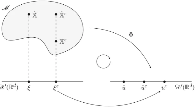
D(Rd)ξε→Xε ∈M, Xε →uε=:(Xε)∈ D(Rd), where(M,d)is a metric space that we call thespace of models. The main point is that the map : M → D(Rd)can be chosen in such a way that its iscontinuous, even thoughM is sufficiently large to allow for elements exhibiting a local scaling behaviour compatible with that ofξ. Of course this means thatξε →Xε is discontinuous in general. In RP, the analogue of the modelXεis the lift of the driving noise as a rough path, the mapis called the Itô-Lyons map, and its continuity (due to T. Lyons [46]) is the cornerstone of the theory. The construction of :M → D(Rd)in the general context of subcritical SPDEs is one of the main results of [32].
The construction of, although a very powerful tool, does not solve alone the aforementioned problem, since it turns out that the most natural choice ofXε, which we call the canonical model, does in general not converge as we remove the regularisation by letting ε → 0. It is necessary to modify, namelyrenormalise, the modelXεin order to obtain a familyXˆεwhich does converge in M as ε → 0 to a limiting model Xˆ. The continuity of then implies thatuˆε:=(Xˆε)converges to some limituˆ :=(Xˆ), which we call therenormalised solutionto our equation, see Fig.1. A very important fact is thatuˆεis itself the solution of arenormalised equation, which differs from the original equation only by the presence of additionallocal counterterms, the form of which can be derived explicitly from the starting SPDE, see [2].
The transformationXε→ ˆXεis described by the so-calledrenormalisation group. The main aim of this paper is to provide a general construction of the space of modelsM together with a group of automorphisms G− S :
M → M which allows to describe the renormalised modelXˆε = SεXε for an appropriate choice ofSε ∈ G−.
Fig. 1 In this figure we show the factorisation of the mapξε→uεintoξε→Xε→(Xε)=
uε. We also see that in the space of modelsMwe have several possible lifts ofξε ∈S(Rd), e.g. the canonical modelXεand the renormalised modelXˆε; it is the latter that converges to a modelXˆ, thus providing a lift ofξ. Note thatuˆε=(Xˆε)anduˆ =(Xˆ)
renormalised model and its convergence as the regularisation is removed are based onad hocarguments which have to be adapted to each equation. The present article, together with the companion “analytical” article [9] and the work [2], complete the general theory initiated in [32] by proving that virtu-ally every1 subcritical equation driven by a stationary noise satisfying some natural bounds on its cumulants can be successfully renormalised by means of the following scheme:
• Algebraic step: Construction of the space of models(M,d)and renormal-isation of the canonical modelM Xε → ˆXε∈M, this article.
• Analytic step: Continuity of the solution map:M → D(Rd), [32].
• Probabilistic step: Convergence in probability of the renormalised model
ˆ
XεtoXˆ in(M,d), [9].
• Second algebraic step: Identification of(Xˆε)with the classical solution map for an equation with local counterterms, [2].
We stress that this procedure works for very general noises, far beyond the Gaussian case.
1 There are some exceptions that can arise when one of the driving noises is less regular than
white noise. For example, a canonical solution theory for SDEs driven by fractional Brownian motion can only be given forH > 14, even though these equations are subcritical for every
[image:10.439.65.378.56.228.2]1.2 Overview of results
We now describe in more detail the main results of this paper. Let us start from the notion of asubcritical rule. Arule, introduced in Definition5.7below, is a formalisation of the notion of a “class of systems of stochastic PDEs”. More precisely, given any system of equations of the type (1.7), there is a natural way of assigning to it a rule (see Sect.5.4for an example), which keeps track of which monomials (of the solution, its derivatives, and the driving noise) appear on the right hand side for each component. The notion of asubcriticalrule, see Definition5.14, translates to this general context the notion of subcriticality of equations which was given more informally in [32, Assumption 8.3].
Suppose now that we have fixed a subcritical rule. The first aim is to construct an associated space of modelsMex. The superscript ‘ex’ stands forextended
and is used to distinguish this space from therestrictedspace of modelsM, see Definition6.24, which is closer to the original construction of [32]. The space
Mex extends M in the sense that there is a canonical continuous injection M →Mex, see Theorem6.33. The reason for considering this larger space is
that it admits a large groupG−exof automorphisms in the sense of [32, Def. 2.28] which can be described in an explicit way. Our renormalisation procedure then makes use of a suitable subgroup G− ⊂ G−ex which leavesM invariant. The reason why we do not describe its action onMdirectly is that although it acts by continuous transformations, it no longer acts by automorphisms, making it much more difficult to describe without going throughMex.
To defineMex, we construct a regularity structure(Tex,G+ex)in the sense of [32, Def. 2.1]. This is done in Sect.5, see in particular Definitions5.26–5.35 and Proposition5.39. The correspondingstructure group G+exis constructed as the character group of a Hopf algebraT+ex, see (5.23), Proposition5.34and Definition5.36. The vector spaceTexis a right-comodule over T+ex, namely there are linear operators
+ex:Tex→ Tex⊗T+ex, +ex :T+ex→ T+ex⊗T+ex,
such that the identity
(id⊗+ex)+ex=(+ex⊗id)+ex, (1.8)
holds both between operators onTexand onT+ex. The fact that the two oper-ators have the same name but act on different spaces should not generate confusion since the domain is usually clear from context. When it isn’t, as in (1.8), then the identity is assumed by convention to hold for all possible meaningful interpretations.
vector spacesTexandT+exare both left-comodules overT−ex, so that G−exacts on the left onTexand onT+ex. Again, this means that we have operators
−ex:H→T−ex⊗H, H∈ {Tex,T+ex,T−ex}
such that
(id⊗−ex)−ex=(−ex⊗id)−ex.
The action of G−exon the corresponding dual spaces is given by
(gh)(τ):=(g⊗h)−exτ, h ∈H∗, τ ∈H, g ∈ G−ex.
Crucially, these separate actions satisfy a compatibility condition which can be expressed as acointeraction property, see (5.26) in Theorem5.37, which implies the following relation between the two actions above:
g(h f)=(gh)(g f), h ∈ H∗, g∈ G−ex, f ∈ G+ex, H∈ {Tex,T+ex},
(1.9) see Proposition3.33and (5.27). This result is the algebraic linchpin of Theo-rem6.16, where we construct the action of G−exon the spaceMexof models. The next step is the construction of the space ofsmoothmodels of the reg-ularity structure(Tex,G+ex). This is done in Definition6.7, where we follow [32, Def. 2.17], with the additional constraint that we consider smooth objects. Indeed, we are interested in the canonical model associated to a (regularised) smooth noise, constructed in Proposition 6.12 and Remark6.13, and in its renormalised versions, namely its orbit under the action of G−ex, see Theo-rem6.16.
Finally, we restrict our attention to a class of models which arerandom, sta-tionaryand have suitable integrability properties, see Definition6.17. In this case, we can define a particulardeterministicelement ofG−exthat gives rise to what we call theBPHZ renormalisation, by analogy with the corresponding construction arising in perturbative QFT [3,24,35,52], see Theorem6.18. We show that the BPHZ construction yields theuniqueelement of G−exsuch that the associated renormalised model yields acenteredfamily of stochastic pro-cesses on thefinitefamily of elements inTexwith negative degree. This is the
algebraicstep of the renormalisation procedure.
This is the point where the companion analytical paper [9] starts, and then goes on to prove that the BPHZ renormalised model does converge in the metric d on M, thus achieving the probabilistic step mentioned above and thereby completing the renormalisation procedure.
and (6.25). There is also apositive twisted antipode, see Proposition6.3, which plays a similarly important role in (6.12). The main point is that these twisted antipodes encode in the compact formulae (6.12) and (6.25) a number of nontrivial computations.
How are these spaces and operators defined? Since the analytic theory of [32] is based ongeneralised Taylor expansionsof solutions, the vector spaceTexis generated by a basis which codes the relevant generalised Taylor monomials, which are defined iteratively once a rule (i.e. a system of equations) is fixed. Definitions5.8,5.13and5.26ensure thatTexis sufficiently rich to allow one to rewrite (1.7) as a fixed point problem in a space of functions with values in our regularity structure. MoreoverTexmust also be invariant under the actions of G±ex. This is the aim of the construction in Sects.2,3and4, that we want now to describe.
The spaces which are constructed in Sect. 5 depend on the choice of a number of parameters, like the dimension of the coordinate space, the leading differential operator in the equation (the Laplacian being just one of many possible choices), the non-linearity, the noise. In the previous sections we have built universalobjects with nice algebraic properties which depend on none of these choices, but for the dimension of the space, namely an (arbitrary) integer numberd fixed once for all.
The spacesTex,T+exandT−exare obtained by considering repeatedly suit-ablesubsetsand suitablequotientsof two initial spaces, calledF1andF2and
defined in and after Definition4.1; more precisely,F1 is the ancestor of Tex
andT−ex, whileF2is the ancestor ofT+ex. In Sect.4we represent these spaces
as linearly generated by a collection of decorated forests, on which we can define suitable algebraic operations like a product and a coproduct, which are later inherited byTex,T+exandT−ex(through other intermediary spaces which are calledH◦, H1andHˆ2). An important difference between T−exandT+exis
that the former is linearly generated by a family of forests, while the latter is linearly generated by a family of trees; this difference extends to the algebra structure:T−exis endowed with aforest productwhich corresponds to the dis-joint union, whileT+exis endowed with atree productwhereby one considers a disjoint union and then identifies the roots.
The content of Sect.4is based on a specific definition of the spacesF1and F2. In Sects.2and3however we present a number of results on a family of
The family of spaces (Fi)i∈I are introduced in Definition 3.12 on the basis of families of admissible forestsAi,i ∈ I. If(Ai)i∈I satisfy Assump-tions 1, 2, 3, 4, 5 and 6, then the coproducts i of Definition 3.3 are coassociative and moreoveri andj fori < j are incointeraction, see (3.27). As already mentioned, the cointeraction property is the algebraic for-mula behind the fundamental relation (1.9) between the actions of G+ex and
Gex
− on T+ex. “Appendix A” contains a summary of the relations between the most important spaces appearing in this article, while “Appendix B” contains a symbolic index.
2 Rooted forests and bigraded spaces
Given a finite setSand a map:S →N, we write
! def
=
x∈S
(x)!,
and we define the corresponding binomial coefficients accordingly. Note that if 1 and2 have disjoint supports, then (1 +2)! = 1!2!. Given a map
π: S → ¯S, we also defineπ: ¯S →Nbyπ(x)=y∈π−1(x)(y). Fork, :S →Nwe define
k
def
=
x∈S
k(x)
(x)
,
with the conventionk = 0 unless 0≤ ≤ k, which will be used through-out the paper. With these definitions at hand, one has the following slight reformulation of the classical Chu–Vandermonde identity.
Lemma 2.1 (Chu–Vandermonde)For every k: S→N, one has the identity
:π
k
=
πk
π
,
where the sum runs over all possible choices ofsuch thatπis fixed.
Remark 2.2 These notations are also consistent with the case where the mapsk
andare multi-index valued under the natural identification of a mapS →Nd
with a mapS× {1, . . . ,∞} →Ngiven by(x)i ↔(x,i).
2.1 Rooted trees and forests
ofT, also called nodes, are denoted byN = NT and edges byE =ET ⊂N2. Since we want our trees to be rooted, they need to have at least one node, so that we do not allow for trees with NT = . We do however allow for the
trivial tree consisting of an empty edge set and a vertex set with only one element. This tree will play a special role in the sequel and will be denoted by
•. We will always assume that our trees are combinatorial meaning that there is no particular order imposed on edges leaving any given vertex.
Given a rooted tree T, we also endow NT with the partial order≤where
w≤vif and only ifwis on the unique path connectingvto the root, and we orient edges inET so that if(x,y)=(x → y)∈ ET, thenx ≤ y. In this way, we can always view a tree as a directed graph.
Two rooted treesT andTareisomorphicif there exists a bijectionι: ET →
ETwhich is coherent in the sense that there exists a bijectionιN: NT → NT such thatι(x,y) =(ιN(x), ιN(y))for any edge(x,y)∈ eand such that the roots are mapped onto each other.
We say that a rooted tree istypedif it is furthermore endowed with a function
t: ET → L, where L is some finite set of types. We think of L as being fixed once and for all and will sometimes omit to mention it in the sequel. In particular, we will never make explicit the dependence on the choice ofLin our notations. Two typed trees(T,t)and(T,t)are isomorphic ifT andT
are isomorphic andtis pushed ontotby the corresponding isomorphismιin the sense thatt◦ι=t.
Similarly to a tree, aforest Fis a finite simple graph (again with nodesNF and edges EF ⊂ NF2) without cycles. A forest Fisrootedif every connected componentT of F is a rooted tree with rootT. As above, we will consider forests that are typed in the sense that they are endowed with a mapt: EF →L, and we consider the same notion of isomorphism between typed forests as for typed trees. Note that while a tree is non-empty by definition, a forest can be empty. We denote the empty forest by either1or.
Given a typed forestF, a subforestA⊂Fconsists of subsetsEA⊂EFand
NA⊂NFsuch that if(x,y)∈ EAthen{x,y} ⊂ NA. Types in Aare inherited fromF. A connected component ofAis a tree whose root is defined to be the minimal node in the partial order inherited fromF. We say that subforests A
andBare disjoint, and writeA∩B= , if one hasNA∩NB= (which also implies thatEA∩EB = ). Given two typed forestsF,G, we writeFGfor the typed forest obtained by taking the disjoint union (as graphs) of the two forestsFandGand adjoining to it the natural typing inherited fromFandG. If furthermore A⊂F andB⊂Gare subforests, then we writeABfor the corresponding subforest of FG.
We fix once and for all an integerd ≥1, dimension of the parameter-space
2.2 Coloured and decorated forests
Given a typed forestF, we want now to consider families ofdisjoint subforests
ofF, denoted by(Fˆi,i >0). It is convenient for us to code this family with a single function Fˆ :EF NF →Nas given by the next definition.
Definition 2.3 Acoloured forestis a pair(F,Fˆ)such that 1. F =(EF,NF,t)is a typed rooted forest
2. Fˆ: EF NF → Nis such that if Fˆ(e) = 0 fore = (x,y) ∈ EF then
ˆ
F(x)= ˆF(y)= ˆF(e).
We say that Fˆ is acolouringofF. Fori >0, we define the subforest of F
ˆ
Fi =(Eˆi,Nˆi), Eˆi = ˆF−1(i)∩EF, Nˆi = ˆF−1(i)∩NF,
as well asEˆ =i>0Eˆi. We denote byCthe set of coloured forests.
The condition on Fˆ guarantees that every Fˆi is indeed a subforest ofF for
i >0 and that they are all disjoint. On the other hand,Fˆ−1(0)is not supposed to have any particular structure and 0 is not counted as a colour.
Example 2.4 This is an example of a forest with two colours: red for 1 and blue for 2 (and black for 0)
(F,Fˆ)=
A2 A1
A3 A4
We then haveFˆ1 = ˆF−1(1)= A1A3andFˆ2= ˆF−1(2)= A2 A4.
The setCis a commutative monoid under theforest product
(F,Fˆ)·(G,Gˆ)=(FG,Fˆ + ˆG) , (2.1)
where colouringss defined on one of the forests are extended to the disjoint union by setting them to vanish on the other forest. The neutral element for this associative product is the empty coloured forest1.
We add nowdecorationson the nodes and edges of a coloured forest. For this, we fix throughout this article an arbitrary “dimension”d ∈Nand we give the following definition.
Definition 2.5 We denote byFthe set of all 5-tuples(F,Fˆ,n,o,e)such that 1. (F,Fˆ)∈Cis a coloured forest in the sense of Definition2.3.
3. One haso: NF →Zd⊕Z(L)with suppo⊂suppFˆ.
4. One hase: EF →Nd with suppe⊂ {e∈ EF : ˆF(e)=0} = EF\ ˆE.
Remark 2.6 The reason whyotakes values in the spaceZd⊕Z(L)will become apparent in (3.33) below when we define the contraction of coloured subforests and its action on decorations.
We identify (F,Fˆ,n,o,e) and (F,Fˆ,n,o,e) whenever F is isomor-phic to F, the corresponding isomorphism maps Fˆ to Fˆ and pushes the three decoration functions onto their counterparts. We call elements ofF dec-orated forests. We will also sometimes use the notation(F,Fˆ)ne,o instead of
(F,Fˆ,n,o,e).
Example 2.7 Let consider the decorated forest(F,Fˆ,n,o,e)given by
n(h)
t(7),e(7) t(8),e(8)
n(i)
t(3)
n(d),o(d)
t(9) n(j),o(j)
t(4)
n(e),o(e)
t(1),e(1) n(b),o(b)
t(2)
t(5) t(6)
t(10),e(10)
t(11) t(12)
t(13),e(13) n(p)
n(m),o(m)
n(l),o(l)
n(k),o(k)
n(g),o(g)
n(f),o(f)
n(c),o(c)
n(a),o(a)
In this figure, the edges in EF are labelled with the numbers from 1 to 13 and the nodes in NF with the letters {a,b,c, f,e, f,g,h,i, j,k,l,m,p}. We set Fˆ−1(1) = {b,d,e, j,k} {3,4,9} (red subforest), Fˆ−1(2) =
{a,c, f,g,l,m} {2,5,6,11,12} (blue subforest), and on all remaining (black) nodes and edges Fˆ is set equal to 0. Every edge has a type t ∈ L, but only black edges have a possibly non-zero decoratione ∈Nd. All nodes have a decorationn∈ Nd, but only coloured nodes have a possibly non-zero decorationo∈Zd ⊕Z(L).
Example2.7is continued in Examples3.2,3.4and3.5.
Definition 2.8 For any coloured forest(F,Fˆ), we define an equivalence rela-tion∼on the node setNFby saying thatx ∼yifxandyare connected inEˆ; this is the smallest equivalence relation for whichx ∼ywhenever(x,y)∈ ˆE.
Definition2.8will be extended to a decorated forest(F,Fˆ,n,o,e)in Defini-tion3.18below.
way. We associate to each typet∈La kernelϕt :Rd →Rand we define the domain
UF
def
=x ∈(Rd)NF : x
v =xw if v ∼w
,
where ∼ is the equivalence relation of Definition 2.8. Then we set Hτ ∈
C∞(UF),
Hτ(xv, v∈ NF)
def
=
v∈NF
(xv)n(v)
e=(u,v)∈EF\ ˆE
∂e(e)ϕ
t(e)(xu −xv), (2.2)
where, forx =(x1, . . . ,xd)∈Rd,n=(n1, . . . ,nd)∈Nd andϕ ∈ C∞(Rd)
(x)n =def
d
j=1
(xj)nj, ∂nϕ=∂xn11. . . ∂n d
xdϕ ∈ C∞(Rd) .
In this way, a decorated forest encodes a function: every node in NF/ ∼ represents a variable inRd, every uncoloured edge of a certain typeta function
ϕt(e)of the difference of the two variables sitting at each one of its nodes; the decorationn(v)gives a power ofxvande(e)a derivative of the kernelϕt(e).
In this example the decoration o plays no role; we shall see below that it allows to encode some additional information relevant for the var-ious algebraic manipulations we wish to subject these functions to, see Remarks3.7,3.19,5.38and6.26below for further discussions.
Remark 2.10 Every forest F = (NF,EF)has a unique decomposition into non-empty connected components. This property naturally extends to deco-rated forests(F,Fˆ,n,o,e), by considering the connected components of the underlying forestFand restricting the colouringFˆ and the decorationsn,o,e.
Remark 2.11 Starting from Sect.4we are going to consider a specific situa-tion where there are only two colours, namely Fˆ → {0,1,2}; all examples throughout the paper are in this setting. However the results of Sects.2and3are stated and proved in the more general settingFˆ →Nwithout any additional difficulty.
2.3 Bigraded spaces and triangular maps
Definition 2.12 For a collection of vector spaces{Vn : n ∈ N2}, we define the vector space
V = n∈
N2Vn ,
as the space of all formal sumsn∈N2vn withvn ∈ Vn and such that there existsk ∈Nsuch thatvn =0 as soon asn2 >k. Given two bigraded spaces
V andW, we writeV ˆ⊗Wfor the bigraded space
V ˆ⊗W =def n∈N2
m+=n
(Vm⊗W)
. (2.3)
One has a canonical inclusionV ⊗W ⊂V ˆ⊗W given by
m
vm
⊗
w
→
n
m+=n
vm⊗w
, vm ∈ Vm, w∈ W.
However in generalV ˆ⊗W is strictly larger since its generic element has the form
n
m+=n
vn
m⊗w
n
, vn
m ∈Vm, wn ∈ W.
Note that all tensor products we consider are algebraic.
Definition 2.13 We introduce a partial order onN2 by
(m1,m2)≥(n1,n2) ⇔ m1≥n1 &m2 ≤n2.
Given two such bigraded spacesVandV¯, a family{Amn}m,n∈N2of linear maps
Amn :Vn → ¯Vm is calledtriangularifAmn =0 unlessm≥n.
Lemma 2.14 Let V andV be two bigraded spaces and¯ {Amn}m,n∈N2a
trian-gular family of linear maps Amn :Vn → ¯Vm. Then the map
Av =def
m
n
Amnvn
∈ m∈N2V¯m, v=
n
vn ∈ n∈N2Vn
Proof Letv=nvn ∈ V andk ∈Nsuch thatvn =0 whenevern2 >k.
First we note that, for fixedm∈N2, the family(Amnvn)n∈N2is zero unless
n ∈ [0,m1] × [0,k]; indeed if n2 > k thenvn = 0, while ifn1 > m1 then
Amn = 0. Therefore the sum
n Amnvn is well defined and equal to some
¯
vm ∈ ¯Vm.
We now prove that v¯m = 0 whenever m2 > k, so that indeed
mv¯m ∈ m∈N2V¯m. Letm2>k; forn2>k,vnis 0, while forn2 ≤kwe haven2 <m2
and therefore Anm =0 and this proves the claim.
A linear functionA:V → ¯Vwhich can be obtained as in Lemma2.14is called
triangular. The family(Amn)m,n∈N2defines an infinite lower triangular matrix
and composition of triangular maps is then simply given by formal matrix multiplication, which only ever involves finite sums thanks to the triangular structure of these matrices.
Remark 2.15 The notion of bigraded spaces as above is useful for at least two reasons:
1. The operatorsi built in (3.7) below turn out to be triangular in the sense of Definition2.13and are therefore well-defined thanks to Lemma2.14, see Remark2.15below. This is not completely trivial since we are dealing with spaces of infinite formal series.
2. Some of our main tools below will be spaces of multiplicative functionals, see Sect.3.6below. Had we simply considered spaces of arbitrary infinite formal series, their dual would be too small to contain any non-trivial multiplicative functional at all. Considering instead spaces of finite series would cure this problem, but unfortunately the coproductsi do not make sense there. The notion of bigrading introduced here provides the best of both worlds by considering bi-indexed series that are infinite in the first index and finite in the second. This yields spaces that are sufficiently large to contain our coproducts and whose dual is still sufficiently large to contain enough multiplicative linear functionals for our purpose.
Remark 2.16 One important remark is that this construction behaves quite nicely under duality in the sense that ifV andW are two bigraded spaces, then it is still the case that one has a canonical inclusionV∗⊗W∗⊂(V ˆ⊗W)∗, see e.g. (3.46) below for the applications we have in mind. Indeed, the dual
V∗consists of formal sumsnv∗n withvn∗ ∈ Vn∗such that, for everyk ∈ N
there exists f(k)such thatv∗n =0 for everyn ∈N2 withn1 ≥ f(n2).
The setF, see Definition2.5, admits a number of different useful gradings and bigradings. One bigrading that is well adapted to the construction we give below is
|(F,Fˆ)ne,o|bi
def
where
|e| =
e∈EF
|e(e)|, |a| =
d
i=1
ai, ∀a ∈Nd,
and |F \(Fˆ ∪F)| denotes the number of edges and vertices on which Fˆ vanishes that aren’t roots ofF.
For any subset A⊆Flet nowAdenote the space built from Awith this grading, namely
A=def n∈
N2Vec{F∈ A : |F|bi=n}, (2.5)
where VecS denotes the free vector space generated by a setS. Note that in generalMis larger than VecM.
The following simple fact will be used several times in the sequel. Here and throughout this article, we use as usual the notation fAfor the restriction of a map f to some subsetAof its domain.
Lemma 2.17 Let V = nVn be a bigraded space and let P : V → V be
a triangular map preserving the bigrading of V (in the sense that there exist linear maps Pn: Vn → Vn such that PVn = Pn for every n) and satisfying
P◦ P = P. Then, the quotient spaceVˆ = V/kerP is again bigraded and one has canonical identifications
ˆ
V = n(Vn/kerPn)= n(PnVn) .
3 Bialgebras, Hopf algebras and comodules of decorated forests
In this section we want to introduce a general class of operators on spaces of decorated forests and show that, under suitable assumptions, one can construct in this way bialgebras, Hopf algebras and comodules.
We recall that(H,M,1, ,1)is abialgebraif:
• H is a vector space overR
• there are a linear map M : H ⊗ H → H (product) and an element
1∈ H (identity) such that(H,M, η)is a unital associative algebra, where
η:R→ H is the mapr →r1(unit)
• there are linear maps : H → H ⊗ H (coproduct) and1 : H → R
(counit), such that(H, ,1)is a counital coassociative coalgebra, namely
• the coproduct and the counit are homomorphisms of algebras (or, equiva-lently, multiplication and unit are homomorphisms of coalgebras).
AHopf algebrais a bialgebra(H,M,1, ,1)endowed with a linear map
A: H → Hsuch that
M(id⊗A)=M(A⊗id)=11. (3.2)
Aleft comoduleover a bialgebra(H,M,1, ,1)is a pair(M, ψ)where
Mis a vector space andψ :M → H⊗Mis a linear map such that
(⊗id)ψ =(id⊗ψ)ψ, (1⊗id)ψ =id. Right comodules are defined analogously.
For more details on the theory of coalgebras, bialgebras, Hopf algebras and comodules we refer the reader to [6,47].
3.1 Incidence coalgebras of forests
Denote by Pthe set of all pairs (G;F) such that F is a typed forest and
G is a subforest of F and by Vec(P) the free vector space generated byP. Suppose that for all(G;F) ∈ Pwe are given a (finite) collectionA(G;F)
of subforests Aof F such thatG ⊆ A ⊆ F. Then we define the linear map
:Vec(P)→Vec(P)⊗Vec(P)by
(G;F)=def
A∈A(G;F)
(G;A)⊗(A;F). (3.3)
We also define the linear functional 1 : Vec(P) → R by 1(G;F) :=
1(G=F). IfA(G;F) is equal to the set of all subforests A of F containing
G, then it is a simple exercise to show that(Vec(P), ,1)is a coalgebra, namely (3.1) holds. In particular, since the inclusion G ⊆ F endows the set of typed forests with a partial order, (Vec(P), ,1) is an example of anincidence coalgebra, see [49,50]. However, ifA(F;G)is a more general class of subforests, then coassociativity is not granted in general and holds only under certain assumptions.
Suppose now that, given a typed forest F, we want to consider not one but several disjoint subforests G1, . . . ,Gn of F. A natural way to code
(G1, . . . ,Gn;F)is to use a coloured forest(F,Fˆ)where
ˆ
F(x)=
k
Then, in the notation of Definition 2.3, we have Fˆi = Gi for i > 0 and
ˆ
F−1(0)=F\(∪iGi).
In order to define a generalisation of the operatorof formula (3.3) to this setting, we fixi >0 and assume the following.
Assumption 1 Leti >0. For each coloured forest(F,Fˆ)as in Definition2.3 we are given a collection Ai(F,Fˆ) of subforests of F such that for every
A∈Ai(F,Fˆ)
1. Fˆi ⊂ AandFˆj ∩A= for every j >i,
2. for all 0< j <iand every connected componentT ofFˆj, one has either
T ⊂ AorT ∩A= .
We also assume thatAi is compatible with the equivalence relation ∼given by forest isomorphisms described above in the sense that ifA∈Ai(F,Fˆ)and
ι:(F,Fˆ)→(G,Gˆ)is a forest isomorphism, thenι(A)∈Ai(G,Gˆ).
It is important to note that colours are denoted by positive integer numbers and are therefore ordered, so that the forests Fˆj, Fˆi andFˆkcan play different roles in Assumption1if j<i<k. This becomes crucial in our construction below, see Proposition3.27and Remark3.29.
Lemma 3.1 Let(F,Fˆ)∈Cbe a coloured forest and A∈Ai(F,Fˆ). Write
• ˆFA for the restriction ofF to Nˆ AEA
• ˆF∪i A for the function on EFNF given by
(Fˆ ∪i A)(x)=
i if x ∈ EANA,
ˆ
F(x)otherwise.
Then, under Assumption1,(A,FˆA)and(F,Fˆ ∪i A)are coloured forests.
Proof The claim is elementary for(A,FˆA); in particular, settingGˆ = ˆdef FA, we haveGˆ j = ˆFj ∩ Afor all j > 0. We prove it now for(F,Fˆ ∪i A). We must prove that, settingGˆ = ˆdef F∪i A, the setsGˆj
def
= ˆG−1(j)define subforests ofF for all j >0. We have by the definitions
ˆ
Gi = ˆFi ∪A, Gˆ j = ˆFj\A, j =i, j>0,
and these are subforests of Fby the properties 1 and 2 of Assumption1.
We denote by Vec(C)the free vector space generated by all coloured forests. This allows to define the following operator for fixedi >0,i :Vec(C)→ Vec(C)⊗Vec(C)
i(F,Fˆ)
def
=
∈ ( ,ˆ)
Note that ifi =1 andFˆ ≤1 then we can identify
• the coloured forest(F,Fˆ)with the pair of subforests(Fˆ1;F)∈ P,
• A(Fˆ1;F)withA1(F,Fˆ)
• in (3.3) with1in (3.4).
Example 3.2 Let us continue Example2.7, forgetting the decorations but keep-ing the same labels for the nodes and in particular for the leaves. We recall that Fˆ is equal to 1 on the red subforest, to 2 on the blue subforest and to 0 elsewhere. Then
(F,Fˆ)= h i j
e
k l m p
A valid example of A∈A2(F,Fˆ)could be such that
(A,FˆA)⊗(F,Fˆ ∪2 A)=
j
e l m
⊗ h i j
e
k l m p
Note that in this example, one has Fˆ2 ⊂ A, so that A ∈/ A1(F,Fˆ)since A
violates the first condition of Assumption1. A valid example ofB∈A1(F,Fˆ)
could be such that
(B,FˆB)⊗(F,Fˆ ∪1 B)=
j i
e
k p ⊗ h i j
e
k l m p
In the rest of this section we state several assumptions on the family
Ai(F,Fˆ) yielding nice properties for the operatori such as coassociativ-ity, see e.g. Assumption2. However, one of the main results of this article is the fact that such properties then automatically also hold at the level of deco-rated forests with a non-trivial action on the decorations which will be defined in the next subsection.
3.2 Operators on decorated forests
The setF, see Definition2.5, is a commutative monoid under theforest product
(F,Fˆ,n,o,e)·(G,Gˆ,n,o,e)=(FG,Fˆ + ˆG,n+n,o+o,e+e) ,
where decorations defined on one of the forests are extended to the disjoint union by setting them to vanish on the other forest. This product is the natural extension of the product (2.1) on coloured forests and its identity element is the empty forest1.
Note that
|F·G|bi = |F|bi+ |G|bi, (3.6)
for anyF,G∈F, where|·|biis the bigrading defined in (2.4) above. Whenever
Mis a submonoid ofF, as a consequence of (3.6) the forest product·defined in (3.5) can be interpreted as a triangular linear map fromM ˆ⊗ M into
M, thus turning(M,·)into an algebra in the category of bigraded spaces as in Definition2.12; this is in particular the case for M =F. We recall that
Mis defined in (2.5).
We generalise now the construction (3.4) to decorated forests.
Definition 3.3 The triangular linear mapsi: F → F ˆ⊗ Fare given for
τ =(F,Fˆ,n,o,e)by
iτ =
A∈Ai(F,Fˆ)
εF A,nA
1
εF A!
n nA
(A,FˆA,nA+πεFA,oNA,eEA)
⊗(F,Fˆ ∪i A,n−nA, o+nA+π(εAF−e A
),eFA+ε F
A) , (3.7)
where
(a) ForA⊆ B⊆ Fand f :EF →Nd, we use the notation fAB
def
= f 1EB\EA.
(b) The sum overnAruns over all mapsnA: NF →Nd with suppnA⊂ NA. (c) The sum overεFA runs over allεFA : EF → Nd supported on the set of
edges
∂(A,F)= {def (e+,e−)∈ EF\EA : e+∈ NA}, (3.8)
that we call theboundary of A in F. This notation is consistent with point a).
(d) For allε :EF →Zd we denote
πε: NF →Zd, πε(x)
def
=
e=(x,y)∈EF
ε(e).
Example 3.4 We continue Examples2.7and3.2, by showing how decorations are modified byi. We consider firsti =2, corresponding to a blue subforest
A∈A2(F,Fˆ). Then we have that(A,FˆA,nA+πεFA,oNA,eEA)is equal to
nA+πεFA,o
nA,o
nA,o
e nA,o
nA,o
nA,o
nA+πεFA,o
nA+πεFA,o
nA,o
nA,o
(3.9)
while(F,Fˆ ∪2 A,n−nA, o+nA+π(εFA−eA),eFA+εFA)becomes
n
e+εF A
e+εF A
n
n−nA,o+nA+πεFA
n−nA,o+nA
n−nA,o+nA
n−nA,o+nA
e+εF
A e+εFA
n n−nA,o+nA
n−nA,o+nA
n,o
n−nA,o+nA+πεFA
n−nA,o+nA+πεFA
n−nA,o+nA
n−nA,o+nA−πe
(3.10)
Note thatεFA is supported by∂(A,F)= {7,8,10,13}, where we refer to the labelling of edges and nodes fixed in the Example2.7, and
πεF
A(d)=ε F A(7)+ε
F
A(8), πε F
A(f)=ε F
A(10), πε F
A(g)=ε F A(13).
Note that the edge 1 was black in(F,Fˆ)and becomes blue in(F,Fˆ ∪2 A);
accordingly, in (F,Fˆ ∪2 A,n−nA, o+nA+π(εFA −eA),eFA +εAF) the value ofeon 1 is set to 0 ande(1)is subtracted fromo(a). In accordance with Assumption1, A∈A2(F,Fˆ)contains one of the two connected components
ofFˆ1and is disjoint from the other one.
Example 3.5 We continue Example3.4for the choice of B made in Exam-ple3.2and fori =1, corresponding to a red subforest B ∈ A1(F,Fˆ). Then
nB(i)
e
nB,o
nB(b),o(b)
nB+πεBF,o
nB,o
nB(p)
nB(k),o(k)
(3.11)
while(F,Fˆ ∪1 B,n−nB, o+nB+π(εFB−eB),eFB+εFB)becomes
n
e+εF B
n−nB,nB
n−nB,o+nB+π(εFB−eB )
n−nB,o+nB
n−nB,o+nB
e n−nB,o+nB
e e
n−nB,nB
n,o n,o n−nB,o+nB
n,o n,o
n,o
n,o
(3.12)
Here we have that∂(B,F) = {7}, where we refer to the labelling of edges and nodes fixed in the Example2.7. ThereforeπεFB(d)=εFB(7). Note that the edge 8 was black in(F,Fˆ)and becomes red in(F,Fˆ ∪1 B); accordingly, in
(F,Fˆ ∪1 B,n−nB, o+nB+π(εBF−eB),eFB+εBF)the value ofeon 8 is set to 0 ande(8)is subtracted fromo(d). In accordance with Assumption1,
B ∈ A1(F,Fˆ) is disjoint from the blue subforest Fˆ2 and, accordingly, all
decorations onFˆ2are unchanged. Finally, note that the edge 1 is not in∂(B,F)
since it is equal to(a,b)withb∈ Banda∈/ B.
Remark 3.6 From now on, in expressions like (3.7) we are going to use the simplified notation
A,FˆA,nA+πεAF,oNA,eEA
=:A,FˆA,nA+πεFA,o,e
,
namely the restrictions ofoandewill not be made explicit. This should generate no confusion, since by Definition2.5in(A,Aˆ,n,o,e)we haveo: NA →
Zd ⊕Z(L)ande: EA→Nd. On the other hand, the notationFˆArefers to a slightly less standard operation, see Lemma3.1above, and will therefore be made explicitly throughout. Note also thatnAisnotdefined as the restriction ofntoNA.
Let us consider first the particular case ofτ =(F,Fˆ,0,o,e). ThennAhas to vanish because of the constraint 0≤nA ≤nand (3.7) becomes
iτ =
A∈Ai(F,Fˆ)
εF A
1
εF A!
(A,FˆA, πεFA,o,e)
⊗(F,Fˆ ∪i A,0, o+π(εAF−eA),eFA+εFA) . (3.13)
Consider a single term in this sum and fix an edge e = (v, w) ∈ ∂(A,F). Then, in the expression
F,Fˆ ∪i A,0, o+π(εAF−eA),eFA+εFA
,
the decoration ofeis changing frome(e)toe(e)+εFA(e). Recalling (2.2), this should be interpreted as differentiatingεFA(e)times the kernel encoded by the edgee. At the same time, in the expression
A,FˆA, πεFA,o,e
,
the termπεAF(v)is a sum of several contributions, among whichεFA(e). If we take into account the factor 1/εAF(e)!, we recognise a (formal) Taylor sum
k∈Nd
(xv)k k! ∂
e(e)+k
xv ϕt(e)(xv−xw), e=(v, w)∈∂(A,F).
Ifnis not zero, then we have a similar Taylor sum given by
k∈Nd
(xv)k k! ∂
e(e)+k xv
(xv)n(v)ϕt(e)(xv−xw)
, e=(v, w)∈∂(A,F).
The role of the decorationois still mysterious at this stage: we ask the reader to wait until the Remarks3.19,5.38and6.26below for an explanation. The connection between our construction and Taylor expansions (more precisely, Taylorremainders) will be made clear in Lemma6.10and Remark6.11below.
Remark 3.8 Note that, in (3.7), for each fixed Athe decorationnA runs over a finite set because of the constraint 0≤nA≤n.
On the other hand,εFA runs over an infinite set, but the sum is nevertheless well defined as an element of F ˆ⊗ F, even though it doesnot belong to the algebraic tensor productF ⊗ F. Indeed, since|eEA| + |eFA +εFA| =
![Outlook and appraisal [October 2005]](data:image/gif;base64,R0lGODlhAQABAIAAAP///wAAACH5BAEAAAAALAAAAAABAAEAAAICRAEAOw==)