Stable and unstable vortex knots in excitable media

Stable and unstable vortex knots in excitable media

Jack Binysh,1_{Carl A. Whitfield,}2_{and Gareth P. Alexander}3,*

1_{Mathematics Institute, Zeeman Building, University of Warwick, Coventry CV4 7AL, United Kingdom} 2_{Division of Infection, Immunity and Respiratory Medicine, University of Manchester, Southmoor Road,}

Manchester M23 9LT, United Kingdom

3_{Department of Physics and Centre for Complexity Science, University of Warwick, Coventry CV4 7AL, United Kingdom}

(Received 12 September 2018; published 16 January 2019)

We study the dynamics of knotted vortices in a bulk excitable medium using the FitzHugh-Nagumo model. From a systematic survey of all knots of at most eight crossings we establish that the generic behavior is of unsteady, irregular dynamics, with prolonged periods of expansion of parts of the vortex. The mechanism for the length expansion is a long-range “wave-slapping” interaction, analogous to that responsible for the annihilation of small vortex rings by larger ones. We also show that there are stable vortex geometries for certain knots; in addition to the unknot, trefoil, and figure-eight knots reported previously, we have found stable examples of the Whitehead link and 62knot. We give a thorough characterization of their geometry and steady-state motion. For the unknot, trefoil, and figure-eight knots we greatly expand previous evidence that FitzHugh-Nagumo dynamics untangles initially complex geometries while preserving topology.

DOI:10.1103/PhysRevE.99.012211

I. INTRODUCTION

Models of excitable media support spiral wave vortices in two dimensions. In a three-dimensional medium the analo-gous structure is a vortex filament [1]. Such a filament may close on itself to form, in the simplest case, an unknotted loop, and more generally a knotted vortex [2]. As well as being or-ganizing centers for waves of excitable activity, early numeri-cal experiments and theoretinumeri-cal work showed that these knot-ted filaments have their own dynamics [3–9]. Remarkably, in a simple example of an excitable medium, the FitzHugh-Nagumo model, simulations suggested that these dynamics were topology preserving, and further that they were capable of “simplifying” a knot, reducing an initially complicated filament geometry to a simpler stationary state [3–5]. Such a scenario stands in stark contrast to the knot untying via reconnection events seen in other examples of knotted fields such as fluids and superfluids [10–12].

So far, the striking knot simplification has been reported only for the unknot [13]—reducing three examples of tangled, but unknotted, curves to a geometric circle of fixed average radius—and, in two examples, the trefoil [13,14]. At higher crossing number the behavior appears to be more complicated. Nevertheless, with the exception of two examples discussed below, reported knot and link evolutions are still consistent with preservation of topology [3–5,13–16]. Stationary states have been reported for all torus knots and links up toN = 12 [15,16], whereN denotes the crossing number of the knot

*_{Corresponding author: G.P.Alexander@warwick.ac.uk}

Published by the American Physical Society under the terms of the

Creative Commons Attribution 4.0 International license. Further distribution of this work must maintain attribution to the author(s) and the published article’s title, journal citation, and DOI.

or link, although only in the case where they are stabilized by proximity to a planar surface with Neumann (no-flux) boundary conditions and the vortex filaments are initialized to have the idealized geometry of torus curves. Both of these features are believed to be important for the stability of these examples [15,16]. If the vortex is initialized with idealized torus geometry but not sufficiently close to the boundary, it is prone to poorly understood instabilities which cause it to deviate from the initially symmetric form. Similarly, torus knots initialized without the idealized geometry do not evolve to the observed stationary states and instead follow irregular dynamics, typically ending with the filament breaking upon contact with the no-flux surface. It is not known how close to the idealized torus geometry the initial curve needs to be to attain the stationary state. A cautionary example is provided by early bulk (not close to a no-flux boundary) simulations of a variety of knots and links, including torus knots, started from exactly symmetric configurations, which appeared stable over the times initially simulated [4]. As we shall demonstrate in the case of torus knots, over longer timescales such geometries in fact destabilize. The recent no-flux simulations are over much longer timescales; however, in the absence of theoretical results it is not clear exactly how long a simulation is “long enough.”

Underlying all of the above observations are general ques-tions as to the driving factors behind knot dynamics, which can be expected to involve both the topology of the vortex and its geometry. Theoretical work has focused on local geometric models of filament motion in which an isolated straight filament is perturbed to have slight curvature and longitudinal twist in the phase of its cross-sectional spiral waves [6–9,19,20]. To lowest order these deformations lead to filament motion with both normal and binormal compo-nents, as well as a modification of vortex rotation frequency away from the intrinsic (straight filament) frequency of the excitable medium [6,8,9]. A “sproing” instability, in which an initially straight filament twisted above some critical thresh-old destabilizes and adopts a helical conformation, has also been predicted and observed [4,6,8,19,20], which has been proposed [15] to account for the deformations seen in torus knot simulations.

These considerations are all local and do not capture the global topology of the vortex or nonlocal wave-vortex interactions, which are essential to the process of simplifi-cation without reconnection observed for unknotted loops. The nonlinear waves of excitation propagating from the vor-tex filament mutually annihilate when they meet, creating a complex “collision interface” [3–5,14,21] depending not only on the filament geometry but also on the synchrony of wave emission from distant parts of the vortex (Ref. [21] shows an example of this interface for a trefoil knot with a different kinetics to that considered here). The analogous structure in a two-dimensional medium, sometimes known as a “shock structure” [22], is well studied in a variety of excitable media [23–28]. If a two-dimensional spiral vortex interacts with a wave field of frequency higher than its own (as generated either by other vortices or externally) this interface moves toward the low-frequency vortex until directly upon it, at which point the high-frequency wave field directly slaps the vortex. This slapping may then induce motion in the vortex, commonly referred to as “spiral wave drift” or “high-frequency induced drift.” The same scenario may occur in three dimensions—a more general instance of the wave-slapping mechanism described above for a pair of coaxial rings—and has been proposed as an important driver of fil-ament dynamics, a conjecture for which there is some indirect evidence [5,14,16]. However, in the three-dimensional case the factors that determine the collision interface are poorly understood—as discussed above, local filament geometry may in principle affect vortex rotation period, but the observed frequency shift and annihilation of a small unknot suggests that interfilament interactions and Doppler shift due to relative filament motion are also important.

We present here the results of a systematic survey of the dynamics of all prime knots up to crossing number N =8 and focus on behavior in the bulk, using periodic bound-ary conditions, so as to further complement recent work by Maucher and Sutcliffe [13,15,16,18], who have studied no-flux boundary conditions. We find generically that knotted vortices do not stabilise into simplified stationary states, al-though some do. The predominant behavior is of unsteady dynamics and instability through the expansion of some por-tion of the knot into a large loop; we present evidence that this instability occurs through the wave-slapping mechanism

alluded to previously. In a substantial fraction of cases (eight of thirty-six), the instability eventually leads to strand recon-nections in the bulk, demonstrating that such events are in fact not exceptional as one increases crossing number and do not occur solely at a boundary or in a highly symmetric geometry. The reconnections are of antiparallel strands, driven together through wave slapping in a manner analogous to the annihilation of the unknot discussed above, and result in links. For both a generic knot and the specific case of idealized torus knots we additionally investigate the role of the sproing instability in knot destabilization, finding it to be unimportant in explaining generic knot instability and not directly responsible for torus knot destabilization, although correlated with torus knots attaining a temporarily stable knot length.

Our survey also shows that for N 4 (unknot, trefoil, figure eight) knots do exhibit topology preserving dynamics toward stationary states. We strengthen these results, and for the unknot those of Ref. [13], by testing the bulk untangling dynamics of all of these knots with a wide variety of initial conditions—in the case of the unknot, a far greater variety than has been used previously. We find that in the bulk a generic unknot, trefoil, or figure eight simplifies to a canonical form, but that the wave-slapping mechanism at play for large N can cause rates of convergence to vary dramatically. We then characterize the geometry and long-term dynamics of these stationary states and two further examples that we have found, a Whitehead link and a 62knot, both of which appear to belong to the same “family” as the figure-eight knot, sharing with it many dynamical properties. This commonality does not cleave across preexisting knot types, for example, torus knots, but rather is a property of the FitzHugh-Nagumo dynamics.

II. METHODOLOGY

A. The FitzHugh-Nagumo model

The FitzHugh-Nagumo model is given by the pair of nonlinear reaction-diffusion equations

∂u ∂t =

1

u−1 3u

3_−v

+ ∇2_u, ∂v

∂t =(u+β−γ v),

(1)

above; the actual radius found in Ref. [17] is 4.8. Over such a length scale, one expects short-range intervortex repulsion in a generic knotted filament.

B. Simulating bulk FitzHugh-Nagumo dynamics

We simulate Eq. (1) with periodic boundary conditions using the pseudospectral method of Ref. [29], in which the linear part of Eq. (1) is solved exactly in Fourier space via an integrating factor, and nonlinear terms are computed via fast Fourier transform. Thereafter, a fourth-order Runge-Kutta timestepping is used. When such a method is employed for diffusive systems, high wave numbers are damped by an expo-nential integrating factor, and the system remains numerically stable for time steps beyond those allowed by the Neumann stability criterion [29]. To test the effects of altering gridspac-ing and timestep we calibrate against the rotation period of a two-dimensional spiral, a quantity known to be sensitive to such choices [30]. We have found that for grid spacings of

x=0.2,0.4,0.6, observing two-dimensional spirals over a time of T =5000 one is able to alter the chosen timestep betweent =0.01 andt=0.14 with no measurable effect on spiral period. In practice, with the exception of simulations to be discussed in Sec.III A, we perform simulations using gridspacingx =0.5, timestept =0.1.

Our use of periodic boundaries complements existing re-sults by removing the effects of no-flux boundary interactions on vortex evolution, allowing us to study long time bulk dy-namics without vortex knots breaking at (or nestling into) the boundary. One might worry that although we have removed boundary interactions they have been replaced by the effects of periodic neighbors. Figure 1(a) shows a snapshot of a typical periodic simulation. The structure of the wave field, shown in orange, is tracked by plotting the level setu=1.6. It has a complex topology at length scales comparable to that of the vortex filament, shown in red. However, further from the filament the shells of wave activity simplify to a series of concentric spheres propagating outward from the location of the filament. This is a consequence of the nonlinear nature of the waves—when two wavefronts meet they fuse, creating a single cusped front, which is then smoothed by the curvature dependence of front propagation velocity. Provided the simulation domain size remains large in comparison to the dimensions of the vortex filament (and noting that, as we shall see, filament dynamics are typically orders of magnitude slower than wave dynamics), these shells shield the vor-tex from its periodic neighbors—the outermost shell passes across the periodic boundary and annihilates itself, leaving the bulk of the simulation untouched. As an example, in Figs.1(b) and1(c)we compare snapshots from two simulations of the same knot evolution, in this case the 72knot, but run in boxes of different sizes. Figure1(b)is identical to Fig.1(a)except that we only show a cross section through the wave field. Figure1(c)shows the corresponding knot and cross section taken from the larger simulation. Considering discrepancies between the two wave fields where they overlap (in other words only in the smaller box) we see that differences are localized to a region on the boundary of the smaller box, with the bulk of the two simulations in agreement on this smaller box. As expected, the knot loci themselves are identical. The

Side length: 174

Side length: 225 (a)

(b)

(c)

data shown is taken at time T =2420 after initialization, O(200) vortex rotation periods into the simulation (why we select this particular knot and simulation snapshot for display will be discussed further in Sec.III), during which time (and throughout the remainder of the simulation) the knots from the smaller and larger simulations track one another perfectly. We may thus be confident that our periodic simulation is indeed capturing bulk behavior. In practice, how large a simulation box one needs to ensure this behavior will vary depending on knot dynamics and the timescale of simulation. For the results presented here, we find a box size of 174 to be sufficient.

C. Defining and tracking the vortex filament

Stacking two-dimensional spiral vortices one obtains the simplest example of a vortex filament, one with a straight ge-ometry from which emanates a quasi-two-dimensional “scroll wave” [1]. More generally, the vortex filament is a tubular structure with arbitrary geometry, normal cross sections of which resemble spiral vortices whose phase is allowed to vary longitudinally. (In fact even this picture is an idealisation; waves emanating from other sections of the filament can disrupt this local spiral wave structure.) Various operational definitions to extract a one-dimensional curve from this tubu-lar structure have been proposed [3,4,30]. Here we follow Refs. [13–16,18] and first compute the intermediate quantity

B=∇u×∇v. (2)

|B| measures the deviation of u and v contours from colinearity—it is zero for a planar wave and only attains substantial nonzero value along the vortex filament. Contours of|B|thus take the form of tubes. For example, Fig.1tracks the vortex filament by showing the level set|B| =0.4 in red. To extract a one-dimensional curve from such a tube, we first note thatBorients the tube. Stepping along the tube in the direction given by this orientation, we connect maximal values of|B|in cross sections taken through it, resampling if necessary to give equidistant steps; a similar extraction proce-dure is detailed in Ref. [3]. This raw curve is then smoothed to remove modes of frequencies comparable to λ, giving a smoothed curve from which we may compute curvatures and torsions via finite difference. (The choice of length scale for filtering is motivated by the observation that the most highly curved stable filament observed, a stable round unknot [17], has a circumference comparable toλ.) Typically we will use the term “filament” to emphasize the one-dimensional curve defined above, and “vortex” when we wish to discuss the full tubular stack of spiral waves surrounding this curve. This definition (and indeed other “instantaneous” definitions [30]) gives rise to small amplitude oscillations in the geometry of the filament at period ∼T₀ which carry through to derived quantities such as knot length. We shall examine the spectrum of these oscillations in detail in Sec.IV, but in subsequent plots showing length evolution we filter them out for clarity.

As discussed above, vortex phase varies along the filament, framing our one-dimensional curve, and the twist of this framing may in principle affect both filament motion and vortex rotation period. We track it by computing _|∇_∇u_u| along the filament and then smoothing as above.

D. Initializing a knotted vortex field

To initialize an arbitrary knotted vortex for simulation we adopt the basic strategy of Refs. [13,14] in which a phase fieldφ(x)∈S1_,x∈R3_{\K, is constructed which contains a} phase singularity with the geometry of some desired vortex knot K. Thereafter, the winding of φ around the specified knotted phase singularity is translated into the winding of (u, v) around the excitation-recovery loop of the FitzHugh-Nagumo model as one encircles the vortex filament via the map (u, v)=(2 cosφ−0.4,sinφ−0.4).

To construct a phase fieldφcontaining a singularity along a given curveK, we first compute the solid angle functionω aboutKusing the formula [31]

ω(x)=

K

n_∞×n·dn

1+n·n_∞ mod 4π, (3)

where for y∈K, n:= _|yy₋−x_x| is the projection of K onto a unit sphere centered onxandn_∞is an arbitrary unit vector. For a discussion of this integral and its numerical properties, including its singular behavior about points x such that n· n∞= −1, we refer the reader to Ref. [31].

The solid angle contains the necessary phase singularity alongK, and for the simulations discussed in this paper we use it for initialization directly by settingφ=ω/2. We briefly note, however, that the structure ofωaboutKdoes not mirror that of a typical (u, v) wave field, which consists of a series of approximately equispaced wavefronts radiating outwards from the vortex filament (Fig. 1). Further, this methodology does not give control over the initial twist distribution along the filament, which is set by the intersection of the level set ω=0 withK, the “solid angle” framing ofK[31]. We may control both of these features by modifyingφas

φ(x)=k₀d(x)+1₂ω(x), (4)

where k0:=2π/λ0 is the spiral wave number and d(x) := miny∈K|y−x| is the minimal distance from x toK.k0d(x) increases linearly with distance from the curve, giving a periodic modulation ofφand hence (u, v) with distance. As an example, Fig.2(a) shows the wave field generated using Eq. (4) whenKis a trefoil knot. The intersection of the level setφ=0 withK, and hence the initial twist distribution, may be controlled by including an offset in the definition ofd(x) which varies alongK. An example of such a modulation, and how it alters the wave field, is shown in Fig.2(b). Given, for example, the importance of twist distribution on both rotation frequency and the sproing instability as discussed above (and further explored in this paper), such control is desirable for future work.

(b) (a)

FIG. 2. Wave-field initialization about a trefoil knot vortex fil-ament (red curve) using Eq. (4), with the level set φ=0 shown in orange. The near half of the level set is clipped to reveal its inner structure. In (a) the definition of d(x) in Eq. (4) is simply minimal distance to the filament. In (b) it is modified by a threefold symmetric sinusoid along the trefoil, effectively adjusting the solid angle framing and local twist rate of the vortex filament.

to one another than the vortex radius λ0/2π, reconnections may occur in the first T ≈T0 of simulation, before the wave field about the knot is established [13]. To ensure this does not occur, given an initialization geometryK we scale isotropically such that the longest side ofK’s bounding box occupies 80% of the simulation box size. As the simulation box isO(50) times the size of the vortex radius, this ensures reconnections do not occur during initialization.

III. UNSTABLE KNOTS

Fascinating recent numerical experiments on the evolution of unknots initialized in complex geometries showed that the FitzHugh-Nagumo dynamics is capable of simplifying an initially tangled unknot to a unique circular curve, without strand crossings [13]. These intriguing examples, coupled with two further instances of simplification in the case of the trefoil [13,14], as well as some indirect evidence of the same behavior for the Hopf link [16] (and a series of preliminary results on various links in Ref. [4]), naturally invite the speculation that such simplification is generic to any knot. To investigate the dynamics of a generic knotted filament, and establish whether this is indeed the case, in Fig.3 we show a survey of the length evolution of all knots up to and including crossing numberN =8, with particular curves that

0 2000 4000 6000

Time 0

200 400 600 800 1000

Length

(a)

0 2000 4000 6000

Time 500

1000 1500 2000 2500 3000

Length

(b)

63 71 72

0 2000 4000 6000

Time 500

1000 1500 2000 2500 3000

Length

(c)

FIG. 3. Length evolution of knotted vortices up to and includ-ing crossinclud-ing numberN =8, with reconnection events indicated by curves which terminate early with a circular marker. Knots included in the legend are further discussed in the text. Note the difference in scale between the first and subsequent panels. (a)N5. (b)N=6 (dotted lines) andN=7 (solid lines). (c)N=8. The unknot (01), trefoil (31), and figure eight (41) settle to a stable length and fixed geometry (see Sec.IV). However, beyond this, generic behavior is an initial period of contraction, followed by length increase over longer timescales. Insets show the geometries resulting from the destabilization of the initially symmetric 51and 71torus knots. we discuss further highlighted in the legend. Excluding chiral variants, there are thirty-six such knots.

T=2419

T=2423 T=2421

T=2417

FIG. 4. Reconnection of the 72knot atT =2423 (orange curve, then orange and green curves after reconnection event) shown in T =2 increments. A pair of antiparallel strands (circled in black) interact, generating a wave field locally similar to that of the stable unknot; shown is the value ofuin a cross section through the knot, with highuvalue colored red. The wave field from the remainder of the knotted filament, shown entering the circled region atT = 2417, impinges upon these strands causing them to destabilize and reconnect. Note that the wave field at T =2420 is also shown in Fig.1.

positive line tension for filaments well separated from any interactions [9]. Our curves are initialized with their strands separated by several vortex radii. Over the first few vortex rotation periods the wave field establishes itself around the vortex filament (over such a timescale the filament may be considered stationary) with the resulting collision interface disjoint from the filament itself. Thereafter each segment of the filament initially moves effectively in isolation from its neighbors.

Over longer timescales, however, we find that this initial contraction does not generically lead filaments to settle to a canonical form or a fixed length, and further that their topology is not always preserved. We observe reconnection events in eight of the thirty-six cases, indicated by those curves terminating in circular markers in Fig.3. The first of these occurs atN =7, with four of the sevenN =7 knots and four of the twenty-oneN =8 knots exhibiting reconnections. Figure 4 shows the reconnection event in the 72 knot occurring atT =2423 inT =2 increments, with the region where the reconnection occurs circled in black. A pair of neighboring antiparallel segments are directly impacted by waves emanating from the rest of the knotted filament, causing them to destabilize and reconnect—the same wave-slapping mechanism responsible for the annihilation of a small unknot by a larger one observed in Ref. [18]. In cross section, the wave field generated by the antiparallel segments (that section

of the wave field ending at the circled antiparallel segments in the T =2417 panel of Fig. 4) locally resembles that of a stable unknot, or indeed of a pair of oppositely signed two-dimensional vortices [17]. However, this stable structure is additionally impinged upon by the wave field of the rest of the knot (shown entering the circled region atT =2417). It has previously been noted that the rotation period of a stable unknot is 14% greater than T0 [18], and as such the stable unknot is vulnerable to wave-slapping-induced annihilation, as it cannot “fend off” a wave train of period T₀. This same argument applies to the antiparallel segments discussed here, but the resulting topological change is reconnection. In addition to the similarity of the wave fields between the coaxial unknots of Ref. [18] and the situation discussed here, the relative filament motion is also the same; in both cases, the perturbed filaments are drifting away from the impinging wave field when topological change occurs. This geometric detail is important, as the velocity of a stable unknot (0.3 [18]) is a substantial fraction of the wave speed in the medium (1.9) and as such Doppler shift may compensate for reduced unknot frequency. For the geometry here, however, the two effects can only compound one another.

Topology changes previously reported in the literature have primarily occurred at simulation boundaries [15,16], and one might be concerned that this reconnection is also an artefact of a finite simulation box. The snapshot of a 72simulation atT = 2420 shown in Fig. 1 was taken from the same data shown in Figs. 3 and4, and was chosen specifically to emphasize that this is not the case. Enlarging the simulation box to side length 225 as shown in Fig.1yields identical knot evolution, including the reconnection event.

Although we have focused the above discussion on the reconnection in the 72 knot, analogous findings hold for the other cases. A detailed understanding of the wave-field evolution leading to such reconnections, and why they are seen here only forN >5, is lacking (we shall see examples of similar wave-field-induced effects for smallN in Sec.IV), but asN increases one generically expects a more complex wave field surrounding the knot as strands become closely packed over one another. As such, we lose the ability to picture segments of the knot as isolated, or even as interacting solely with a unique “nearest-neighbor” region, but instead must think of them analogously to the vortex ring buffeted by external waves.

T ≈4000, and is not evident for the 71 even byT ≈6000, although the inset curve geometries demonstrate the knot has indeed destabilized (that such destabilization occurs, but only after long time simulations, clearly demonstrates the necessity of simulating for many hundreds of rotation periods before drawing conclusions about the dynamics of this system). In the next section, we shall investigate the mechanisms of both the dramatic length increases seen in a generic knot, and of the deviation of the torus knots away from initializations of high symmetry.

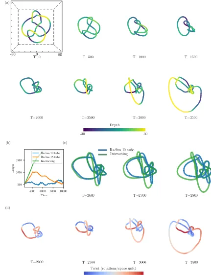
The mechanism of vortex knot length increase

Exploring the knot geometries corresponding to the generic length increases seen in Fig. 3 one finds that, despite the variety of behavior across knots, the increase occurs via a common mechanism in which isolated strands of the knot rapidly expand outwards from a tightly packed core region forming the rest of the knot. We illustrate this behavior for the example of the 63 knot in Fig. 5(a). The same wave-slapping mechanism driving reconnection events has also been proposed as a nonlocal mechanism for persistent knot length increase; in this context when the collision interface intersects a section of the knot, wave-vortex interactions drive that section outwards [5,14]. The interaction does not have an intrinsic length scale, as waves in the medium do not decay. Instead, its range depends upon the geometry of the knot and the accompanying collision interface. For the 63knot shown in Fig.5one may verify that this surface intersects the expanding arm, suggesting that wave slapping may be at play.

Given the potential importance of this mechanism, we would like to establish that it is really driving knot expan-sion, rather than simply being correlated with it. To do so, we investigate the effects of abruptly removing long-ranged interactions entirely, by numerically encasing the filament in a “glass tube” of moderate radius which moves with the filament and fuses when two knot segments approach one another [2]. With this construction, short-range interfilament repulsion and geometry-mediated (including twist-induced) filament motion are preserved but long-ranged interactions are cut out. Using it, we may compare the evolution of a filament both with and without long-range interactions. A suitable radius for the tube is suggested by previous estimates of vortex radius in the literature, as well as the naive estimate λ0/2π ≈3.4: Ref. [17] directly measures a stable vortex ring radius of 4.8, suggesting a vortex radius of∼5, and Ref. [15] estimates a radius of 5.9 by matching ideal rope length [33] and measured trefoil lengths. To implement this construction numerically we simulate only within a tube of lattice points about the filament (the filament itself being constructed as in Sec.II C). In principle the details of the boundary conditions between the vortex and tube must be considered; however, we have found that provided we use a tube radius above the vortex size estimates above, such details do not alter the geometry driven motion of the vortex, a reflection of its localized nature. This observation allows us to sidestep a sophisticated finite-element scheme (the spectral method discussed in Sec.II B only being valid for a periodic box), and instead simply use a finite difference method, with (u, v) values for points outside of the tube set to their fixed point values (−1.03,−0.66). The

tube must move with the vortex; however, we note that this need only happen on the (slow) timescale of vortex motion; we may allow motion in a fixed tube for a timeO(T0), after which the tube is recentered around the vortex. The points brought into the tube at its boundary during this procedure, which had been set to fixed point values, are now allowed to evolve. In practice we typically use a conservative tube radius of∼10 with gridspacingx =0.5 and timestept =0.01, with a finite difference scheme in which the Laplacian is computed using a seven point stencil and both reaction and diffusion terms are evolved using fourth order Runge-Kutta timestepping. The timestep above is chosen as it gives results identical to those of the spectral method usingt=0.1 when measuring the two-dimensional spiral vortex period.

Figure 5(b) contrasts the length evolution of the fully interacting 63knot with a copy of it encased in the tube, with initial conditions for both taken atT =2500, midway through knot expansion. Upon removing long-ranged interactions we no longer see a dramatic increase in knot length. Instead, the length of the tubed knot stabilizes at∼400–600. The details of this stabilization vary depending on the radius of the tube, but the final lengths obtained are approximately the same across radii. Using the core size estimate of Ref. [15], the ideal rope length of the 63 knot is 340 [33], and thus the tubed knot is relatively tightly packed. Over longer timescales [T =8000 shown for the radius 10 tube of Fig.5(b)] the tubed 63does not reach a fixed geometry, but rather undergoes a compact tumbling motion, as the binormal component of filament motion causes segments of the knot to work over one another, though without further substantial length change. In Fig. 5(c) we explore the initial divergence in geometry between the fully interacting and tubed knots. We see that it does not occur globally but is localized to distinct expanding segments of the interacting 63, which lie separate to the knot core region and are responsible for global length increase; these same segments are those which intersect the collision interface. Within the core region, segments of the filament are packed closer than the spatial cutoff we have defined, and there is no immediate divergence between the interacting and tubed knots. By contrast, removing long-range interactions allows distant segments of the tubed knot to evolve under their intrinsic dynamics, unaffected by wave-vortex interactions, and so shrink toward the core region. Thus, a wave-slapping mechanism accounts for global changes in knot length and also for the geometry of where they occur.

T=2600 T=2700 T=2800 Radius 10 tube

Interacting

(a) (b)

we may also examine the twist distribution along the fully interacting filament during knot expansion. Figure5(d)shows this distribution for the 63 knot; we see that the expanding arm of the filament consistently has twist values well below the sproing threshold and, further, that other sections of the knot are more highly twisted, yet do not show the same length increase. In fact, twist values along the entirety of the knot are consistently below the sproing threshold, an observation also made for the early short time simulations of Refs. [4,5].

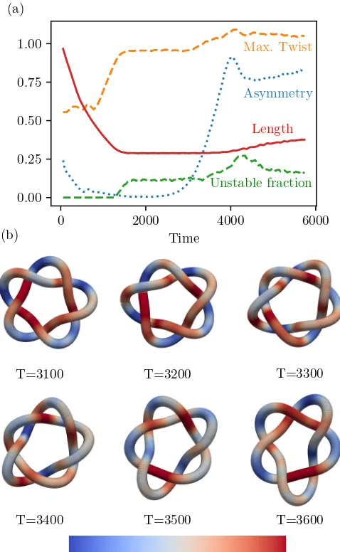
Although not a driver of generic knot length increase, this last observation suggests that the sproing threshold may still have dynamical importance as a stabiliser against curvature induced length decrease, or play a role in the destabilization of symmetric torus knots. In Fig.6we study the destabilization of the 51 torus knot, originally presented in Fig.3, in more detail. Figure6(a) shows the evolution of a measure of the asymmetry of the knot, defined by taking the power spectrum of the knot’s curvature as a function of arclength, and comput-ing the fraction of the power in modes which do not respect the underlying symmetry (fivefold in this case). Alongside it we show the evolution of both the maximal twist, expressed as a fraction of the 0.024 rotations per space unit sproing threshold discussed above, and the fraction of the arclength of the 51which attains a twist greater than 90% of this threshold. We first note that the order of events is broadly consistent with the sproing threshold playing a role in the dynamics. After an initial period in which the knot flattens and the twist remains roughly constant, maximal twist increases until it attains the sproing threshold, thereafter remaining constant; this threshold is attained as the length of the 51 stabilizes. However, it is several hundred rotation periods before we see the subsequent loss of symmetry. This timescale suggests that it is not the case that the knot hits the sproing threshold, and then destabilizes; Ref. [4] notes that the timescale for sproinging to occur is typically only a few rotation periods. Furthermore, the geometry of the destabilization is inconsis-tent with sproing instability. In Fig.6(b)we show the knot as it destabilizes, colored by twist. We fail to see helical sproinging along the highly twisted segments of the knot; instead the whole form collapses to a twofold symmetric shape. A similar deformation is seen in the 71 (see inset of Fig. 3) and has been noted in early simulations of initially symmetric triply linked rings [4], where its cause was attributed to an interplay between the sproing threshold and interfilament interactions. Overall, then, it appears the sproing threshold acts to halt knot shrinkage, but that subsequent destabilization cannot be directly attributed to the sproing instability.

IV. STABLE KNOTS

In Sec.IIIwe showed that the speculation that a generic knotted vortex might simplify to a canonical form—a specu-lation previously evidenced by promising “untangling” results for the unknot [13] and a few further examples of simplifica-tion in low-crossing-number knots and links [14,16]—is not borne out for N >4. In the search for stable knots, recent numerical experiments found that knots and links could be stabilized through proximity to a no-flux boundary [14,15]. Primarily the examples shown were for torus knots and links, although the figure-eight knot and Borromean rings were

T=3100 T=3200 T=3300

T=3400 T=3500 T=3600

0 2000 4000 6000

Time 0.00

0.25 0.50 0.75 1.00 (a)

Length

Asymmetry Max. Twist

Unstable fraction

0.013Twist (rotations/space unit)0.024

(b)

FIG. 6. The role of the sproing instability in the destabilization of the 51torus knot. Panel (a) shows the (normalized) length evolution of the 51, alongside a measure of its asymmetry. Shown also is the maximum absolute twist along the knot as a fraction of the 0.024 rotations per space unit sproing threshold, and the fraction of arclength which attains 90% of this threshold. The twist threshold is reached as knot length plateaus, but no sproinging instability is observed; instead, the knot gradually destabilizes over several hundred rotation periods. Panel (b) shows the geometry of the knot destabilization, colored by twist. Rather than a helical instability developing in regions of high twist, the whole knot transitions to a twofold symmetric form.

0 1000 2000 3000 4000 5000 Time

0 200 400 600 800 1000

Length

(a)

0 2000 4000 6000 8000

Time 200

400 600 800 1000

Length

(b)

0 2500 5000 7500 10000 12500 15000 17500 20000

Time 200

400 600 800 1000 1200 1400

Length

(c) Instability Contraction Tumbling

0 0

17500 2000

FIG. 7. Untangling dynamics of the (a) 18 unknots, (b) 17 trefoils, and (c) 9 figure-eight knots formed by performing single strand crossings on the higher crossing number knot geometries of Sec.III. (a) All unknots simplify to a unique round geometry without reconnection events. Length decrease is monotonic, however there is some variation; the geometry of one particularly slow decay is shown in the inset, displayed at times indicated by the solid markers. (b) All trefoil geometries simplify to a unique stable state, however there is greater variation across decays than for the unknots, with periods where knot length actively increases (boxed inset, circled markers). (c) Of the 9 tangled figure eights simulated, 7 settle rapidly to a stable state. However, overT =20 000 one example fails to converge and another converges only after going through prolonged periods of length increase, contraction, and irregular “tumbling” dynamics.

analogously to the unknot. The states are the same as those found in the survey of Fig.3 and also appear to be the same as those found near a reflecting boundary. In addition, we strengthen the results of Ref. [13] and demonstrate them to be independent of a no-flux boundary by testing the bulk untangling dynamics of the unknot with a far greater variety of initial conditions than has been used previously.

All knots may be converted into the unknot by performing strand crossings. The minimal number of strand crossings needed to convert a knot into the unknot is called its un-knotting number. Of the knots withN 8 there are 18 with unknotting number 1; that is, they can be converted to the unknot by a single strand crossing. By analogous single-strand crossings one can also target the trefoil or figure-eight knots: ForN 8 there are 17 that convert to the trefoil and 9 to the figure eight under a single strand crossing. Beginning with the knot geometries of Sec.III, we use these crossings to provide an assortment of initial tangled geometries for unknots, trefoils, and figure eights, and study their evolution. Figure7(a)summarizes the results of these simulations for the tangled unknots. We find in all cases that the initially tangled vortex transforms to a unique stable ring and that the dynamics does not involve any reconnections. The typical dynamics is an approximately constant rate of length contraction, although

this is not rigorous and there is some variation. In particular, in one example (obtained from the 811knot) there is a substantial period of pause where length decreases much more slowly than is seen on average; snapshots of the geometric evolution of this curve are shown as insets.

fluctuates erratically before eventually settling to the final steady state. The total time that this dynamics plays out over greatly exceeds that of the typical unknot.

These results bridge the gap between the simplification of the unknot discussed in Ref. [13] and our own findings for high-crossing-number knots by showing that, although clearly neither the untangling dynamics nor the geometries giving rise to wave-slapping instability are fully understood, the same mechanisms dominating high-crossing-number knot behavior also play an important role in determining low-crossing-number behavior; wave slapping can totally disrupt the appealing picture of a dynamics which monotonically de-creases knot length even when a stable target state exists. The results also demonstrate the importance of initial conditions on long-term knot evolution; even given the existence of a stable state, the difference between a “good” and “bad” initial starting state may lead to an order of magnitude difference in the time taken to reach that stable state.

Another notable example of the importance of initial conditions comes from the observation that the boundary stabilized trefoil knot actually exists in two distinct stable configurations [15]. The first, which we denote the 31,1, has the geometry that the tangled trefoils of Fig. 7 evolve to. The second, which we denote the 31,2, is not reached by our tangled trefoils. This state was constructed in Ref. [15] from an exactly twofold symmetric initial vortex filament, and preserves this symmetry in the final reported state. Although, as we have seen with torus knots, highly symmetric boundary stabilized states may not exist in the bulk, in our own sim-ulations we have found the 31,2 to be accessible in the bulk using an initial configuration with only approximate twofold symmetry, and have confirmed its stability up toT =12 000. Thus, although this twofold symmetric 31,2 indeed appears stable, the results of our tangled trefoil simulations suggest that it has a small basin of attraction. Taken together, the above results suggest that, although we have seen that the stability of higher crossing number knots is not the norm, stable geometries may nevertheless exist in the bulk, but that when hunting for them we should not use any carelessly chosen initial configuration, but ought to be more selective in which initial geometries we use. For hints as to what those geometries might be, we now investigate in detail the properties of the stable knots we have found thus far.

Properties of stable knots

Figure8shows the geometries, curvature, and torsions as a function of arclength, vortex framings, and twist distributions of the stable 31,1, 31,2 and figure-eight knots. The evolution of their vortex framings at four successive intervals over a (approximate) vortex rotation period are indicated by the vector fields along the curves. Curvatures and torsions shown correspond to the geometries in the far left,T =0 panels (as discussed in Sec.II Cthere is slight intraperiod oscillation), with the arbitrary zero of arclength fixed to coincide with maximal curvature values. We first note the striking twofold symmetry of both the 31,2 and the figure eight knots; this symmetry is not a remnant of initial conditions, but emerges from the underlying dynamics. By contrast, the 31,1 lacks any threefold symmetry. This is especially notable given that

this state was reached starting from an exactly threefold symmetric torus knot geometry in Sec.III. It appears that the boundary stabilized trefoil reported in Ref. [15] also lacks threefold symmetry, although it is unclear why this loss of symmetry does not occur for boundary stabilized torus knots of higher crossing number. A second striking feature of these stable knots is the tight synchronization of the evolution of their framings. The framings of closely separated segments of the filament mesh [4], the wave tip emanating from one segment being consistently met by a wave tip emanating from a spatially neighboring segment, resulting in traveling waves of tightly synchronised wave activity running the length of the knot in a periodic fashion. The pattern is evident in the 31,2and figure-eight knots but is also present in the 31,1, most clearly when one focuses on one of its three relatively straight segments; the framing of the curved lobes is twisted such that it meets the rotation of the wave tip emanating from the straight segment. Again, this meshing is an emergent property of the stable knot.

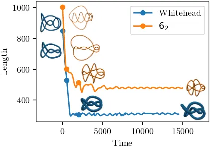
The similarity of the geometries and vortex framings of the 31,2and figure eight is suggestive of a recurrent structural motif. To investigate further we take the geometry of the the stable figure eight and use it as a starting point to construct new trial initialization geometries. We do so in the simplest way possible—as highlighted in the dotted circle around a section of theT =0 figure eight in Fig.8, the knot geometry contains a half-turn of a helix, which we may extend to an integer number of half-turns. Doing so gives a family of trial initialization curves alternating between knots and two component links, the next two being the Whitehead link and the 62knot. Simulation reveals that such initialization geome-tries evolve to apparently stable states. Figure8shows their detailed geometry, and in Fig.9we confirm their bulk stability up toT =15 000. Both states share the twofold symmetry and tight synchronization over a vortex rotation period found in the 31,2and figure-eight knots, with especially close similarity in the geometry and twist distributions of the figure eight, Whitehead link, and 62 knots. This similarity suggests that they arise as the start of a family of such stable knots which does not cleave along some existing subcategory of knots (for example torus knots) but rather arises specifically from the FitzHugh-Nagumo dynamics. As another demonstration of the importance of initial conditions, and a reminder that such states may have small basins of attraction, we note that the 62of Sec.IIIdoes not find this stable state over the times simulated.

T=6 T=9 0 200 Length

0 0.13

Curvature

-0.7 0.7

Torsion

T=3 T=0

0 200

Length

0 0.13

Curvature

-0.7 0.7

Torsion

0 200

Length

0 0.13

Curvature

-0.7 0.7

Torsion

0 100

Length

0 0.13

Curvature

-0.7 0.7

Torsion

1 2

Twist (rotations/space unit) 0.025 -0.025

3_1,1

31,2

4 (figure eight)1

Whitehead link

0 500

Length

0 0.13

Curvature

-0.7 0.7

Torsion

6₂

0 5000 10000 15000 Time

400 600 800 1000

Length

Whitehead

62

FIG. 9. Length evolution of the Whitehead link and the 62knot with initialization geometries made by extending the structure of the stable figure eight knot. Insets correspond to marked times.

structure with knot size, of the drift velocities resembles that found for torus links in Ref. [16]: Within the family of knots discussed above, we see drift velocity decreasing with knot size. However, the complex geometries of the stable knots discussed here renders the explanation for this decrease given for torus knots (decreasing asymmetry between inner and outer parts of the torus as size increases) inapplicable. A reflection of this complexity is that, beyond consistency of scale, there is no clear accompanying pattern in the rotation rate data.

We briefly note that in the above discussion of vortex rotation sense, drift velocity and overall knot rotation sense we have not been careful to distinguish the possibly different behaviours of oriented or chiral variants from one another. All stable knots and links discussed above are isotopic to themselves under reversal of the orientation of any link com-ponent, however, with the exception of the figure eight they are all chiral, and this chirality determines the rotation sense of the knot. In Figs. 8 and 10 we present variants rotating in a right-handed sense about their drift velocity; left-handed variants, with reversed twist distributions, also exist.

As discussed in Sec.III, Ref. [18] reports an increase in the rotation period of a stable unknot by 14%. We investigate whether similar shifts exist for other stable knots by looking at the spectra of their high-frequency length oscillations. Figure10(d)shows the spectra of all stable knots as measured overT =4000 after they reach their stable configurations, alongside the spectra of the firstT =1000 of the unknot and figure eight data shown in Fig.3. We include this second set of data for calibration and methodology validation, as during this time we expect the data to give the spectrum of a nonin-teracting knot, which should approximately correspond tof0. As expected, the length oscillations of the noninteracting data are consistent with the fundamental vortex rotation frequency off₀ =0.0898, and do not vary with knot topology—before intervortex interactions occur the global structure of the fil-ament does not dramatically affect vortex rotation period. In fact, as this data is taken during the contraction of both knots, the observation that it shows purely spectral broadening suggests a negligible role for curvature in possible shifts to rotation frequency. As with the noninteracting data, the stable

knot spectra show single peaks, but their frequencies are shifted relative to the noninteracting case on a scale which exceeds our estimate of curvature induced corrections. For all nontrivial knots, this shift is to a higher frequency (lower period), and its size is approximately constant; we obtain a period of T =0.97T0. By contrast, the unknot alone shows a substantial shift to lower frequencies (higher period); we find an unknot rotation period ofT =1.19T0, consistent with the results of Ref. [18]. That the situation for nontrivial knots is a shift to lower period relative to an isolated filament is intriguing, and suggests itself as a potential origin of the motion of the collision interface leading to the wave slapping observed in Sec.III. One important complicating factor in this sort of analysis is Doppler shift. Although the period of the stable unknot is higher thanT0, its velocity is 0.3, a substantial fraction of the wave speed (1.9) in the medium. Using the data presented here this gives a Doppler shifted period for a sta-tionary observer ahead of the unknot of only 1% greater than T0; in other words, at least for the unknot, relative filament motion is extremely important in determining the stability of a situation. A similar calculation for an observer behind the figure eight gives a Doppler shifted period ofT =0.975T₀, a far less substantial shift. We speculate that these two facts, first, that stable structures generically appear to have periods shifted belowT0, and second, that even when the shift is to a higher period in the case of the unknot (extrapolating unknot behavior to that of generic antiparallel strands) this increase is compensated for in a directional manner by Doppler shift, give an intrinsically unstable dynamics in which the formation of any interacting structure hinders further formation via wave slapping.

V. DISCUSSION

0.074 0.076

Frequency 0

1 2 3 4

Power (filled circles)

1e8

0.088 0.090 0.092 0.094 0 1 2 3 4

Power

(hollow

circles)

1e7 f0

01

01non-interacting 31, 1

31, 2 41

41non-interacting

Whitehead link 62

T=4000 T=2000

T=0

centre of mass fitted helix 01 31, 1 31, 2 41Whitehead62 0.00

0.01 0.02 0.03 0.04 0.05

Speed (o)

0.30

0.000 0.001 0.002 0.003 0.004 0.005 0.006

Rotation rate (rot/space unit) (x

)

(a) (b)

(d) (c)

T=0

T=3000

T=6000

centre of mass

FIG. 10. Dynamics of stable knots. (a) A summary of drift speeds and rotation rates for all known stable knots. Note that the velocity given for the 31,1is that along its helical axis. (b) Drift and rotation of the 62knot. Shown are centers of mass taken atT =100 intervals (blue dots), and snapshots of the geometry atT =3000 intervals; between each snapshot the knot has rotated∼20 times. (c) The 31,1drifts along a helical path (fitted red curve), rotating about the helix axis as a rigid body. (d) Power spectra of high-frequency oscillations in knot length data. Before intervortex interactions occur, the oscillation period is the same asf0. All nontrivial stable knots show a similar shift to higher vortex rotation frequencies (T =0.97T0), with the unknot alone showing a shift to lower frequencies (T =1.19T0).

their associated wave fields, their motion through the medium and natural rotation periods, and shifts in the spectra of their high-frequency length oscillations. In addition to the already known trefoil and figure-eight knots, we found stable forms for the Whitehead link and 62 knot, both of which appear to come from the same “family” of knots as the figure eight. While in the former case, the basin of attraction appears to be large, the same cannot be said for the latter, at least for the timescales of the simulations we have run.

Throughout this paper, we have emphasized the importance of the collision interface on understanding long timescale vortex dynamics. Although we have seen many examples of its importance, an understanding of its own dynamics is currently qualitative at best. As a first step toward rectifying this, it would be interesting to directly study the evolution of local rotation rate along a vortex to fully disentangle the possible effects of curvature, twist, and interactions. Turning from general dynamical questions to the details of stable states, beyond noting close similarities between those found

we have not proposed principles by which their geometry and behavior may be understood. A detailed description appears challenging, but the observed wave-field synchronization, and similarities in the size of spectral shifts, of Sec.IVoffers a global organizing principle from which one might try to pre-dict geometries. When discussing stability we have contrasted our own results in the bulk with those on torus knots and links that have been found near no-flux boundaries [15,16], detailing where results overlap (the stability of the trefoil and figure eight) and where they diverge. Although we have seen that boundary stabilization is more complex than simply a suppression of the sproing instability, its exact nature remains unclear and deserves further study.

gave two-dimensional vortices with desirable properties and three-dimensional simulations were computationally feasible. It would be interesting to revisit these choices armed with new criteria for a desirable set of parameters. For example, we might search for parameters (or indeed models) such that rotation frequency is seen to decrease with twist and interactions. A related question is to explore whether wave-slapping interactions have any role in enhancing untangling as well as hindering it—in other words, whether the untangling aspect of the dynamics can be captured in a local geometric model. Here the tubed knot of Sec. III offers some hints; in preliminary simulations of tubed versions of the tangled unknots of Sec.IVwe do not see substantial differences in the untangling times between tubed and untubed unknots. It may be the case that, although the full dynamics appear extremely difficult to capture with a local geometric model, such a model offers insight for the restricted case of unknot untangling. This is especially interesting given the apparent contrast between the untangling dynamics seen here and those utilized by line tension minimization methods [13].

Stable vortex rings have been realised experimentally and successfully described using existing theory [35–37]. As such, although one expects the precise details of knot stability to be specific to the system studied, we believe that our explo-ration of the phenomena seen here—the importance of wave slapping, bulk simplification of low-crossing-number knots, frequency shifts in stable knots—is of direct experimental interest for a general excitable medium, outside of the details of the FitzHugh-Nagumo model.

ACKNOWLEDGMENTS

We are grateful to P. Sutcliffe for useful discussions. J.B. acknowledges partial support from a David Crighton Fellowship and thanks R. E. Goldstein for his discussions on spectral methods, as well as his and DAMTP’s hospital-ity during the fellowship. This work was supported by the UK EPSRC through Grants No. EP/L015374/1 (J.B.) and No. EP/N007883/1 (C.A.W. and G.P.A.).

[1] A. T. Winfree and S. H. Strogatz, Singular filaments organize chemical waves in three dimensions: I. Geometrically simple waves,Physica D8,35(1983).

[2] A. T. Winfree and S. H. Strogatz, Singular filaments orga-nize chemical waves in three dimensions: III. Knotted waves, Physica D9,333(1983).

[3] A. T. Winfree, Stable particle-like solutions to the nonlinear wave equations of three-dimensional excitable media, SIAM Rev.32,1(1990).

[4] C. Henze, Vortex filaments in three dimensional excitable me-dia, Ph.D. thesis, The University of Arizona, 1993.

[5] A. T. Winfree, inNonlinear Dynamics and Chaos: Where do we go from here?, edited by S. J. Hogan (IoP, London, 2002). [6] J. P. Keener, The dynamics of three-dimensional scroll waves in

excitable media,Physica D31,269(1988).

[7] J. P. Keener and J. J. Tyson, The dynamics of scroll waves in excitable media,SIAM Rev.34,1(1992).

[8] H. Dierckx, Dynamics of wave fronts and filaments in anisotropic cardiac tissue, Ph.D. thesis, The University of Ghent, 2010.

[9] V. N. Biktashev, A. V. Holden, and H. Zhang, Tension of organizing filaments of scroll waves,Phil. Trans. R. Soc. Lond. A347,611(1994).

[10] M. W. Scheeler, D. Kleckner, D. Proment, G. L. Kindlmann, and W. T. M. Irvine, Helicity conservation by flow across scales in reconnecting vortex links and knots,Proc. Natl. Acad. Sci. USA111,15350(2014).

[11] D. Kleckner and W. T. M. Irvine, Creation and dynamics of knotted vortices,Nat. Phys.9,253(2013).

[12] D. Kleckner, L. H. Kauffman, and W. T. M. Irvine, How superfluid vortex knots untie,Nat. Phys.12,650(2016). [13] F. Maucher and P. Sutcliffe, Untangling Knots Via

Reaction-Diffusion Dynamics of Vortex Strings, Phys. Rev. Lett. 116, 178101(2016).

[14] P. M. Sutcliffe and A. T. Winfree, Stability of knots in excitable media,Phys. Rev. E68,016218(2003).

[15] F. Maucher and P. Sutcliffe, Length of excitable knots,Phys. Rev. E96,012218(2017).

[16] F. Maucher and P. Sutcliffe, Dynamics of linked filaments in excitable media,arXiv:1804.07064.

[17] M. Courtemanche, W. Skaggs, and A. T. Winfree, Stable three-dimensional action potential circulation in the FitzHugh-Nagumo model,Physica D41,173(1990).

[18] F. Maucher and P. Sutcliffe, Rings on strings in excitable media, J. Phys. A: Math. Theor.51,055102(2018).

[19] H. Henry and V. Hakim, Scroll waves in isotropic excitable media: Linear instabilities, bifurcations, and restabilized states, Phys. Rev. E65,046235(2002).

[20] B. Echebarria, V. Hakim, and H. Henry, Nonequilibrium Ribbon Model of Twisted Scroll Waves,Phys. Rev. Lett.96, 098301(2006).

[21] C. Henze and A. T. Winfree, A stable knotted singularity in an excitable medium,Int. J. Bifurcat. Chaos1,891(1991). [22] L. N. Howard and N. Kopell, Slowly varying waves and shock

structures in reaction-diffusion equations,Stud. Appl. Math.56, 95(1977).

[23] V. I. Krinsky and K. I. Agladze, Interaction of rotating waves in an active chemical medium,Physica D8,50(1983).

[24] E. A. Ermakova, V. I. Krinsky, A. V. Panfilov, and A. M. Pertsov, Interaction of spiral and flat periodic autowaves in an active medium, Biofizika31, 318 (1986).

[25] M. Vinson, Interactions of spiral waves in inhomogeneous excitable media,Physica D116,313(1998).

[26] G. Gottwald, A. Pumir, and V. Krinsky, Spiral wave drift induced by stimulating wave trains, Chaos 11, 487 (2001).

[27] K. Agladze, M. W. Matthew, V. I. Krinsky, and N. Sarvazyan, Interaction between spiral and paced waves in cardiac tissue, Am. J. Physiol. Heart. Circ. Physiol.293,H503(2007). [28] S. Dutta and O. Steinbock, Spiral defect drift in the wave

[29] R. E. Goldstein, D. J. Muraki, and D. M. Petrich, Interface proliferation and the growth of labyrinths in a reaction-diffusion system,Phys. Rev. E53,3933(1996).

[30] M. Dowle, R. M. Mantel, and D. Barkley, Fast simulations of waves in three-dimensional excitable media, Int. J. Bifurcat. Chaos7,2529(1997).

[31] J. Binysh and G. P. Alexander, Maxwell’s theory of solid angle and the construction of knotted fields,J. Phys. A: Math. Theor. 51,385202(2018).

[32] R. Scharein,http://knotplot.com/.

[33] T. Ashton, J. Cantarella, M. Piatek, and E. J. Rawdon, Knot tightening by constrained gradient descent,Exp. Math.20,57 (2011).

[34] P. Enkhbayar, S. Damdinsuren, M. Osaki, and N. Matsushima, HELFT: Helix fitting by a total least squares method,Comp. Bio. Chem.32,307(2008).

[35] T. Bánsági and O. Steinbock, Nucleation and Collapse of Scroll Rings in Excitable Media,Phys. Rev. Lett.97,198301 (2006).

[36] A. Azhand, J. F. Totz, and H. Engel, Three-dimensional autonomous pacemaker in the photosensitive Belousov-Zhabotinsky medium,Europhys. Lett.108,10004(2014). [37] J. F. Totz, H. Engel, and O. Steinbock, Spatial confinement