Hierarchical Bayesian method for detecting continuous gravitational waves from an ensemble of pulsars

ensemble of pulsars

SUPA, School of Physics & Astronomy, University of Glasgow, Glasgow G12 8QQ, United Kingdom

X. Fan‡

Department of Physics & Astronomy, Hubei University of Education, 430205 Wuhan, China (Dated: September 7, 2018)

When looking for gravitational wave signals from known pulsars, targets have been treated using independent searches. Here we use a hierarchical Bayesian framework to combine observations from individual sources for two purposes: to produce a detection statistic for the whole ensemble of sources within a search, and to estimate the hyperparameters of the underlying distribution of pulsar ellipticities. Both purposes require us to assume some functional form of the ellipticity distribution, and as a proof of principle we take two toy distributions. One is an exponential distribution, defined by its mean, and the other is a half-Gaussian distribution defined by its width. We show that by incorporating a common parameterized prior ellipticity distribution we can be more efficient at detecting gravitational waves from the whole ensemble of sources than trying to combine observations with a simpler non-hierarchical method. This may allow us to detect gravitational waves from the ensemble before there is confident detection of any single source. We also apply this method using data for 92 pulsars from LIGO’s sixth science run. No evidence for a signal was seen, but 90% upper limits of 3.9×10−8 _{and 4.7×10}−8 _{were set on the mean of an assumed exponential ellipticity}

distribution and the width of an assumed half-Gaussian ellipticity distribution, respectively.

PACS numbers: 02.50.Ng, 04.80.Nn, 95.55.Ym, 95.85.Sz, 97.60.Gb

I. INTRODUCTION

So far, Advanced LIGO [1] and Advanced Virgo [2] have detected gravitational waves from the time vary-ing mass quadrupole caused by the orbital motion of two compact objects: binary systems consisting of two black holes [3, 4] or two neutron stars [5]. However, individ-ual neutron stars with deformations can also have a time varying mass quadrupole that is not detectable as a tran-sient signal with a chirplike nature, but is long-lived and quasimonochromatic. From such sources, the expected gravitational wave signal strength at Earth is given by[6]

h0≈4.2×10−24

f2 kHz

Dkpc

Izz 1038_{kg m}2

ε

10−6

, (1)

wherefkHz is the star’s rotation frequency in kHz,Dkpc

is its distance in kpc, and the combination of the fiducial ellipticity [7], ε = |Ixx−Iyy|

Izz , and principal moment of

inertia,Izz, are related to the mass quadrupole moment (based on the definition of [8]) by

Q22=

r 15

8πIzzε. (2)

Galactic neutron stars that are observed as pulsars are an enticing target for such signals. The times of ar-rival of electromagnetic pulses from pulsars can, in many

∗_{matthew.pitkin@glasgow.ac.uk} †_{christopher.messenger@glasgow.ac.uk} ‡_{fanxilong@outlook.com}

cases, be used to fit their phase evolution to great ac-curacy. This leads to high precision measurements of the spin frequency and frequency derivative, often sub-milliarcsecond position reconstruction, and for sources in multiple systems, estimates of their orbital parameters. Under the assumption that any pulsar’s mass quadrupole is formed by its having a triaxial moment of inertia el-lipsoid (or, more colloquially, a “hill,” “mountain,” or “bump”), and that the rotation is phase locked with the electromagnetic emission, then the gravitational wave signal will be at exactly twice the observed frequency. Therefore, the precise phase evolution of any associated gravitational wave signal can be used as a filter for the signal in gravitational wave data. The only unknowns in the signal model are therefore the gravitational wave amplitude at Earth, as given in Eq. (1), and the ori-entation of the pulsar given by the inclination angle, ι, polarization angle,ψ, and relative phase at the epoch of the electromagnetic timing model,φ0. As in, e.g., [6, 9–

13], following the method of [14], Bayesian inference can be used to produce a joint posterior probability density function on these four parameters, and the orientation parameters can be marginalized over to give a posterior on only h0. If the distance to a pulsar is known then

this can be used to make inferences on, or set a limit on, the mass quadrupole moment,Q22, or alternatively, the

pulsars fiducial ellipticity assuming a canonical moment of inertia ofIzz = 1038kg m2 [7].1

In previous searches for known pulsars in gravitational

1_{The canonical moment of inertia is roughly what you get from}

wave data from the LIGO, Virgo and GEO600 detectors [6, 9–13] no signal has been seen, but upper limits, at a 95% credible level, were set on h0 for all included

pul-sars. In the latest results [13], using data from the first observing run (O1) of the advanced LIGO detectors [15], this produced limits onh0for 200 pulsars, which in turn

gave limits onQ22 andεusing the best-fit measured

dis-tances given in the ATNF Pulsar Catalogue [16]. The lowest limits on Q22 and ε found for any pulsar were

9.7×1029_{kg m}2 _{and 1.3}

×10−8 _{respectively, for the}

rela-tively nearby (∼0.2 kpc) pulsar PSR J0636+5129. Different neutron star equations of state can allow dif-ferent sizes of deformations to be sustained in the star; stiffer equations of state allow larger deformations than softer ones. A good review of themaximumallowed ellip-ticities is given in [7], which shows that in very extreme cases they could be in the range of 10−3_{, but more}

real-istically, for crustal deformations, they could reach a few ×10−6_{. Internal magnetic fields can also induce an}

ellip-ticity in a neutron star (e.g., [17]), with field strengths of order 1015_{G required to give rise to ellipticities of}

∼10−6_{. For known pulsars, assuming their rate of loss}

of rotational energy is all due to gravitational wave emis-sion, one can infer the ellipticity required to give the ob-served spin-down (called the “spin-down limit”). For the population of millisecond pulsars, such maximum pos-sible ellipticities are generally well above the spin-down limit, which give values in the range∼10−9

−10−8_{. So,}

it is fair to assume that this population of pulsars is not strained to their maximum allowed values. The recent work in [18] provides some tentative evidence that mil-lisecond pulsars may actually have aminimumellipticity of∼10−9_.

Searches for gravitational waves from pulsars have al-ways treated each pulsar individually. However, as we will describe further in this paper, it is possible to com-bine observations from many pulsars to try and detect the ensemble of all pulsars used in a search. The idea is that there may be several sources that are individually below some allowed threshold for detection, but when combined the ensemble rises above a detection thresh-old. This was proposed in [19], in which values of the_F -statistic [20], commonly used in continuous gravitational wave searches, for individual sources are summed. The method of [19] depends rather sensitively on the relative strengths of the brightest few sources, and is unlikely to be able to detect an ensemble of similar strength but indi-vidually undetectable, sources, i.e., it does not “win” by much over single source searches. This idea was extended in [21] to weight the individual_F-statistic values based on the expected detectability of each source, i.e., favor-ing close-by sources, which was found to always provide a more sensitive detection statistic than [19].

In this paper we also address the task of combining an

assuming a uniform density spherical star with a mass of 1.4 M and radius of 10 km.

ensemble of sources, but for two purposes: to try and es-timate the functional form of the underlying distribution of pulsar ellipticities, and to use the combined sources as an ensemble detection method. The former of these could allow us to make some physical inferences about the equation of state, or internal magnetic field strength, of the population of neutron stars. The latter, as discussed above, could allow us to detect the ensemble before an individual source is confidently detected.

II. METHOD

Our aim is to combine data from all pulsars within a gravitational wave signal search to try and estimate the underlying distribution of their fiducial ellipticities (or alternatively, Q22). We can do this within the context

of hierarchical Bayesian inference, whereby we use the data to infer parameters of a probability distribution that represents the prior on the ellipticities (in this context these parameters are often calledhyperparameters). This is essentially the same underlying method as described in [22], where in that context the main use is for detecting a stochastic background of compact binaries coalescences that are individually unresolvable.

In previous searches, each pulsar has been treated indi-vidually, and a posterior distribution on the gravitational wave amplitude,h0, has been estimated, via

p(h0|xi, I)∝ Z θi

p(xi|h0,θi, I)p(h0|I)p(θi|I)dθi, (3)

wherexiis the data for theith pulsar,θi={cosι, φ0, ψ}i are the pulsar’s orientation parameters,p(xi|h0,θi, I) is the likelihood ofxigiven the signal model and particular parameter values,p(θi|I) is the prior probability on the

θi parameters (which is flat over the allowed parameter ranges, see Sec. 3.2 of [23]), andp(h0|I) is the prior on

h0. More recently, in [13], the marginal likelihood (or

Bayesian evidence) for each pulsar’s data being consistent with the expected signal model has also been calculated, via

p(xi|I) =

Z θiZ h0

p(xi|h0,θi, I)p(h0|I)p(θi|I)dθidh0.

(4) The prior on h0 has often been flat between zero and

some hard upper cutoff, or having a Fermi-Dirac-like dis-tribution (see, e.g., Sec. 2.3.5 of [24]) with a flat section followed by an exponential-like decay at some predefined value.

Alternatively, we can rearrange Eq. (1), and for each pulsar we can estimate the joint posterior onεi and the pulsar’s distance,Di,

p(εi, Di|xi, I) =

p(εi|I)

Zi Z θi

p(xi|εi, Di,θi, I)

where Zi ≡p(xi|I) is the evidence of the data (we will use the termevidence, rather thanmarginal likelihood in the rest of this paper as it is more compact). To produce a posterior onεi we need to set the priors for Di andεi. We can use a Gaussian prior on Di defined by a mean valueµDi, taken as the best-fit estimate from the ATNF

Pulsar Catalogue [16] (which is generally a dispersion measure-derived distance based on the galactic electron density model of [25]), and a standard deviation,σDi,

2

p(Di|µDi, σDi, I) =

1 √

2πσDi

exp

−(Di−µDi)

2

2σ2

Di

. (6)

For each pulsar the distance is independent, and as the distances are not of interest to us, we can marginalize over them in Eq. (5) as nuisance parameters.3

The prior on εi can be a function that represents the underlying distribution of pulsar ellipticities. We will say that the function is defined by a set of parameters, which in this context are called the hyperparameters, Θ that are intrinsic to the pulsar population. We can combine likelihoods for allNpulsars in a search, where for each we marginalize over the parametersθi,Di, andεi, leaving a likelihood forΘ,

p(X_|Θ, I) = N Y

i

Z εiZ θiZ Di

p(xi|εi,θi, Di, I)p(θi|I)p(εi|Θ, I)p(Di|µDi, σDi, I)dεidθidDi. (7)

where X_{≡ {}xi} means the combined data from all pul-sars.4 _{We are interested in estimating the parameters of}

the underlying ellipticity distribution,Θ, and also calcu-lating the evidence for the data given our particular cho-sen ellipticity distribution. To do this we further need to define a prior onΘand apply Bayes theorem,

p(Θ_|X, I) =p(Θ|I)p(X|Θ, I)

p(X_|I) , (8)

where the evidence is

p(X_|I) = Z Θ

p(X_|Θ, I)p(Θ_|I)dΘ. (9)

The posterior onΘallows us to estimate the distribu-tion ofε, while we can use the evidence,p(X_|I), for the hypothesis that the data is consistent with that particu-lar distribution to perform model selection. For example,

2 _{Throughout this work we will take the distance uncertainty to}

be 20% of theµDi value, which is roughly what Figure 12 in

[26] suggests for dispersion measure-based distance estimates. For some pulsars better distance estimates are available (using, for example, parallax measurements obtained using very long baseline interferometry), while for others the uncertainties can be considerably worse, so in a detailed analysis more reliable uncertainties could be used for individual pulsars.

3 _{For pulsars in the same globular cluster the distance}

measure-ments and error would essentially be the same, or at least very highly correlated, but we will ignore that fact in this study. Of the pulsars currently listed in the ATNF Pulsar Catalogue [16] with rotation frequencies above 10 Hz, 139 of the 451 pulsars are in globular clusters. The clusters with the largest numbers of pulsars are 47 Tucanae, with 25, and Terzan 5, with 35.

4 _{It is worth emphasizing that even though the same raw data is}

used for all pulsars, the precise signal and the Gaussian compo-nent of the colored noise spectrum for each pulsar will be en-tirely independent. Tracking the signal’s precise phase over a long (weeks, months, or years) observation time means that the phase templates for different sources (even if there were billions of sources!) are highly orthogonal.

we could calculate the ratio of this evidence to one where the hypothesis is that the data for all pulsars consists purely of noise, i.e. the Bayes factor or odds (assuming prior odds of unity), and use this as a detection statistic for the ensemble of sources.

A. Ellipticity distribution priors

We study two different toy models for the underlying ellipticity distribution: an exponential distribution de-fined only by its mean,µε,

p(ε|µε, I) = 1

µε

e−ε/µε ₍₁₀₎

such that Θ _≡ µε; and, a half-Gaussian distribution peaking at zero, and defined by its width,σε,

p(ε_|σε, I) = 2 √

2πσε

e−ε2_/2σ2

ε, (11)

such thatΘ_≡σε. We note that more attention is given to the exponential model in most of our examples.

We also need to set a prior on Θ for both cases. For both models we chose a prior on the hyperparameter that is uniform in log-space between some lower and upper bounds, e.g., for the exponential distribution we have

p(µε|I) = [ln (µεmax/µεmin)] −1 1

µε

, (12)

and equivalently for σε. For the analyses described in Sec. III we use a lower bound of 10−10 _{and an upper}

bound of 10−5_.

likely gone through a stage of accretion (see, e.g., the review in [27]) that spins them up and reduces their ex-ternal dipole magnetic field.5 _{This could mean that the}

distribution of ellipticities for these two populations may be quite different, and therefore a bimodal distribution, or two independent exponential distributions with differ-ent means, could be more appropriate. Alternatively, it may be more appropriate to use a quasinonparametric approach, such as the histogram binning in [28], an infi-nite Gaussian mixture model (see, e.g., [29] for a recent example of this in the context of gravitational waves), or a Gaussian process to model the ellipticity distribu-tion funcdistribu-tion space. All these approaches have largerΘ parameter spaces to marginalize over and are therefore computationally more challenging. We leave the explo-ration of these ideas to future work.

B. Using posterior samples

If we have many pulsars, e.g., the 200 used in [13], and wanted to directly calculate Eqs. (8) and (9) then it would require integrals over 200×4 independent param-eters (θi ={cosι, φ0, ψ}i and Di for each pulsar), and a large data set consisting of the data for each pulsar. How-ever, as those parameters and the noise in each pulsar’s gravitational wave data are independent, we can calcu-late the likelihood overεifor each pulsar individually, as is already done for current targeted pulsar searches [13]. This simplifies Eq. 7 to be

p(X_|Θ, I) = N Y

i Z εi

p(xi|εi, I)p(εi|Θ, I)dεi. (13)

In reality those searches do not output a functional form of the likelihood for each pulsar, but they use nested sampling [30] to compute the evidence that the data con-tains a signal (coherently combined over multiple de-tectors), p(xi|I), and produce samples drawn from the marginalized posteriordistributionp(εi|xi, I). The pos-terior samples therefore need to be converted into a func-tional form of the likelihood for use in Eq. (8).6

First, to convert these samples into a smooth func-tional form we can use kernel density estimation (KDE), with a Gaussian kernel. To remove edge effects for sam-ples that rail against the lower bound of zero we reflect all

5 _{Current searches for gravitational waves from pulsars [13]}

con-sider all pulsars with rotation frequencies above 10 Hz. Within this subset of∼450 pulsars, as given by the ATNF Pulsar Cat-alogue [16], about 50 of them have high spin-down rates and as such would be considered “young”, while the rest are old recycled pulsars.

6 _{In reality the software that performs the nested sampling [24]}

and outputs the posterior samples usesQ22 rather thanε, but

we can easily convert between the two using Eq. (2) and assuming a principal moment of inertia of 1038_{kg m}2_.

the samples about zero and concatenate these with the original samples before performing the KDE. When eval-uating the resulting KDE only at allowed positive values ofεit must then be multiplied by two to get the correct probability density.

Next, rearranging Bayes theorem shows how to turn a posterior for an individual pulsar into a likelihood

p(xi|εi, I) =

p(εi|xi, I)

p(εi|I)

p(xi|I), (14)

where in this caseεiis the prior onεused for the individ-ual pulsar. If the priorp(εi|I) is uniform (i.e. a constant) in some range within which the likelihood goes to zero then this is simple to calculate. In all our examples this is the case, with εi being defined between zero and an upper rangeεmax, such that

p(εi|I) =ε−max1 . (15)

To be explicit, we are undoing an effective uniform prior that was used when calculating the original pulsar pos-teriors, so that we can then reapply our new ellipticity distribution prior for the whole ensemble. We can there-fore substitute

p(xi|ε,I) =εmaxp(εi|xi, I)p(xi|I), (16)

into Eq. (7). We could also work with samples in h0

rather than ellipticity, and numerically marginalize over distance errors, which we show in Appendix A, but we will not useh0samples in this paper.

We have found that in our analysis, when we have many posteriors that peak at, or close to, zero, and a prior function that increases rapidly as it approaches zero, we cannot use the method as used in, e.g., [28]. That method approximates the integral over the likeli-hood multiplied by the prior with the expectation value of the prior evaluated at each of the samples. We find that the accuracy of this approach is significantly reduced for small values of prior parameters likeµε(see Sec. II A above) when there are no samples with roughly equiva-lent values.

C. Spin-down limits

We could use the electromagnetically-derived spin-down limits described briefly in Sec. I to infer the hyper-parameters of our ellipticity distribution. For each pul-sar we have a spin-down limit onεbased on its observed electromagnetic spin-down, independent of the pulsar’s distance (combining Eqs. (5) and (6) of [12])

εsd₌ 1.9×10−8

f_kHz5/2

|f˙rot|

10−11_{Hz s}−1

!1/2

1038_{kg m}2

Izz

1/2

.

proper motion effects (the Shklovskii effect [31]), differ-ential galactic rotation [32], and, for pulsars in globular clusters, local accelerations. Indeed, these effects lead to some pulsars being observed to spin-up. Therefore in any inference using spin-down limits one would have to either correct for these effect, or exclude pulsars for which the effects cannot be estimated.

We can use these spin-down limit derived values to provide a likelihood on εi for each pulsar when estimat-ing the underlyestimat-ing distribution’s hyperparameters. For an individual pulsar we can (simplistically) say that the spin-down limit gives us a flat likelihood onε

p(dEMi|εi, I) = (

1/εsd

i if 0≤εi≤εsdi ,

0 otherwise (18)

where dEMi is the electromagnetically derived informa-tion, i.e., from observed pulse time of arrivals, that gives the spin-down limit for a given pulsar.

These likelihoods for each pulsar can be combined into a joint likelihood, and form a likelihood on the distribu-tion’s hyperparameters, Θ,

p({dEM}|Θ, I) =

N Y

i Z

p(dEMi|εi, I)p(εi|Θ, I)dεi

.

(19) If we assume the underlying distribution is exponential (so Θ_≡µε) we have

p(_{dEM}|µε, I) = N Y

i ₁

εsd

i

Z εsd_i

0

1

µε

e−εi/µε_dε

i, (20)

where we can see that the integral is just the cumula-tive distribution function for an exponential distribution, which is given by CDF(εsd

i , µε) = 1−e− εsd

i /µε_{. So, we}

have

p(_{dEM}|µε, I)∝ N Y

i

1₋e−εsd

i /µε_{. (21)}

A similar result can be found for the half-Gaussian dis-tribution using its CDF.

Using the priors given in Sec. II A we can calculate the posteriorsp(µε|{dEM}, I) andp(σε|{dEM}, I) for the

ex-ponential and half-Gaussian distributions, respectively. To do this we use all pulsars in the ATNF Pulsar Cat-alogue [16], excluding those in globular clusters and with observed spin-ups, estimate their intrinsic period derivatives (by calculating the combined Shklovskii and galactic rotation effects using best-fit distances from the catalogue), and calculate their spin-down limits using Eq. (17). For this simple analysis we ignore uncertain-ties in each pulsar’s moment of inertia. The posterior probability distributions on µε and σε for the exponen-tial and half-Gaussian are shown in Fig. 1. We find 90% credible upper bounds on these two hyperparameters of

µ90%

ε ≤3.0×10−10 andσε90%≤4.1×10−10.

10−10 ₁₀−9 ₁₀−8 ₁₀−7 ₁₀−6 ₁₀−5

µε/σε 104

105 106 107 108 109

Probabilit

y

Densit

y

Exponential Half-Gaussian Prior

FIG. 1. The posterior probability distributions on the el-lipticity distribution prior hyperparameters µε and σε for

the exponential and half-Gaussian distributions when using electromagnetically-derived spin-down limits.

In the rest of this paper we will purely assume the use of gravitational wave data alone for making inferences about the ellipticity distribution. However, an interest-ing extension to this work could be combininterest-ing the gravi-tational wave data for pulsars, where that places a more stringent limit than the spin-down limit, with spin-down limits for the pulsars where it does not.

D. Bayes factor

We saw in Eq. (9) that we can calculate the evidence that the data is consistent with a particular parameter-ized ellipticity distribution (i.e., the exponential or half-Gaussian distributions). However, to make this number informative we need to be able to compare it to another model. We can form the odds between this evidence and one given by a different hypothesis, such as the data from all pulsars being entirely consistent with Gaussian noise, e.g.

Oε

n=

p(X_|Hε, I)

p(X_|Hn, I)

p(Hε|I)

p(Hn|I)

, (22)

1. Noise hypothesis

The simplest way to form the evidence for the noise hy-pothesis is just as the product of the null likelihoods for all pulsars, where the null likelihood is the likelihood with the signal model explicitly set of zero (see, e.g., Sec. 2.2.3 of [24] for the null likelihoods used in the analysis pre-sented here). For a particular pulsariand detectorjthe null likelihood for the hypothesis that the data is consis-tent with noise alone,Hn, is given by

p(xj_i|Hnj, I)≡p(x

j

i|εi= 0, I), (23) i.e., it is just the likelihood [as seen in, e.g., Eq. (5)] eval-uated with the signal model set to zero. Therefore, with xi≡ {xji}, the multidetector (Ndet) noise hypothesis for

a single pulsar is

p(xi|Hn, I) =

NYdet

j

p(xj_i|Hnj, I), (24)

and evidence for the noise hypothesis for all pulsars is

p(X_|Hn, I) =

Y

i

p(xi|Hn, I). (25)

In reality such a noise hypothesis is not robust against instrumental spectral disturbances and lines in the data (see, e.g., [33]), which can contaminate the frequencies near, or at, those of an expected astrophysical pulsar signal. If data from more than one detector is avail-able, a more robust noise hypothesis is to allow it to incorporate incoherent signals or noise between detec-tors. When using multiple detectors, the individual pul-sar signal hypothesis enforces coherence between them, so we can more explicitly call the hypothesis the coher-ent hypothesis, Hcoh, which is what the evidence term

p(xi|I)≡p({xji}|Hcoh, I) in Eqs. (5), (14) and (16) truly

represents.

The evidence for the new noise hypothesis for each pulsar, which we will call the incoherent hypothesis, is described in more detail in Sec. 2.6 of [24], or the Ap-pendix of [13]. In all the analyses presented here we use two detectors (the LIGO Hanford and Livingston detec-tors, which we will denote as H1 and L1 respectively from here onwards), so for each pulsar the evidence for the in-coherent hypothesis,Hin is

p(xi|Hin) =

Y

j∈{H1,L1}

h

p(xj_i|Hj

s, I) +p(x

j i|H

j

n, I)

i

, (26)

whereHj

s is the evidence for the hypothesis that the data

is consistent with a signal for a single detector. This is generalizable to any number of detectors. Again, we can take the product of this to give the incoherent hypothesis for allN pulsars

p(X_|Hin) =

N Y

i

p(xi|Hin). (27)

This implies that in Eq. (22) we would substitute Hn≡

Hin, which is the case for all results presented here.

2. Nonhierarchical statistic

Without using any of the machinery in defining an underlying ellipticity distribution, and hyperparameters, described previously in this section, we can form a more na¨ıve odds. This assumes all the pulsars have mass quadrupoles (not ellipticities) drawn from the same flat prior distribution with fixed bounds (between zero and a large value at which all likelihoods have approached zero). To differentiate it from the above odds formed using an ellipticity distribution with unknown hyperpa-rameters, we call this ournonhierarchical statistic.

As described above, for each pulsar we have the evi-dence for the coherent signal modelp({xj_i}|Hcoh, I) and

the null likelihoodp(xi|Hn, I). Following a similar route

to Eqs. (49–52) of [34] we can form the probability (not the evidence here as we are explicitly including priors on the hypotheses) for a compound hypothesis of any com-bination of individual signal and noise hypotheses

p(Hcom|X, I)∝

N Y

i h

p(xi|Hcohi, I)p(Hcohi|I)+

p(xi|Hini, I)p(Hini|I) i

− N

Y

i

p(xi|Hini, I)p(Hini|I), (28)

where p(Hcohi|I) and p(Hini|I) are the priors for each hypothesis, which here we explicitly state for each pulsar

i. The second product term on the right-hand side of Eq. (28) is also the probability for the all-pulsar noise hypothesis, so we can produce an odds between the two probabilities (noting that they would both have the same proportionality coefficient and it would thus cancel out) as

O ≡p_p(₍H_Hcom|X, I)

in|X, I)

= p(X|Hcom, I)

p(X_|Hin, I)

p(Hcom|I)

p(Hin|I)

= N Y

i h

p(xi|Hcohi, I)p(Hcohi|I)+

p(xi|Hini, I)p(Hini|I) i!

×

N Y

i

p(xi|Hini, I)p(Hini|I) !−1

−1. (29)

hypotheses, e.g.,

N Y

i=1

p(Hini|I) =

N Y

i=2

p(Hini|I) 1

Y

j=1

p(Hcohj|I)

= N Y

i=3

p(Hini|I)

3

Y

j=1

p(Hcohj|I)

=. . . , (30)

then Eq. (29) becomes

O= QN

i [p(xi|Hcohi, I) +p(xi|Hini, I)] QN

i p(xi|Hini, I)

−1, (31)

where implicitly p(Hcom|I) = (2N −1)p(Hin|I).

There-fore, to assign equal prior odds for the compound hy-pothesis that data for any pulsar contains a signal one must use

ONH

n =

O

2N ₋₁. (32)

We will use this as a comparison to Eq. (22) in the sub-sequent analyses.

3. B-statisticlike comparison

It is interesting to compare the above statistics to that proposed in [19]. Due to how we have constructed our data sets, it is not simple to calculate the _F-statistic (which is the log-likelihood ratio maximized over the parameter space) for our simulated data for each pul-sar. However, the natural logarithm of our signal versus noise evidence ratios for each pulsar are essentially the B-statistic of [35] (although we additionally marginalize over pulsar distance) including the line robust incoherent noise denominator [33] in our Bayes factors. Therefore, as a comparison using an ensemble of pulsars, we can simply sum these_B-statistics. In our notation, where we are not implicitly in log-space, we would have a product rather than a sum of

OB

n =

N Y

i

p(xi|Hcohi, I)

p(xi|Hini, I)

. (33)

As was shown in [35] the_B-statistic is a slightly more effi-cient discriminator between signal and noise than theF -statistic, so we would expect this to produce a compara-ble, but slightly more efficient statistic than that in [19]. On a final note, all the above likelihood, prior, poste-rior, and odds calculations are in practice computed en-tirely using the natural logarithm of the values to avoid numerical underflow and overflow.

III. ANALYSIS

Here we will discuss analyses that have been performed on simulated data to assess the performance of the three

odds given in Eqs. (22), (31) and (33) for detecting an ensemble of gravitational wave signals from pulsars. In the former case this assumes that all pulsars have ellip-ticities drawn from some underlying distribution defined by unknown hyperparameters, while the latter two as-sume no unknown hyperparameters for the distribution. In the former case we also assess how well we can recover the hyperparameters defining the ellipticity distribution.

A. Simulations

To make these assessments we have produced a series of simulated data sets to account for different ellipticity distributions, hyperparameter values, and for different realizations of noise. In all cases we take the 200 pulsars searched for in the analysis of LIGO Observing Run 1 (O1) [13] as our sample of sources, with their sky po-sitions and best-fit distances obtained from the ATNF Pulsar Catalogue [16]. We also create data from two detectors, the LIGO Hanford (H1) and Livingston (L1) observatories, assuming that they are operating at their advanced design sensitivities [36, 37] over one year with a 100% duty cycle. For each pulsar a complex time series is simulated at a sample rate of once per 1800 s, to repli-cate the data that would be produced in a real targeted pulsar search (e.g., [13]) following the application of a heterodyne procedure [14] to remove the rapidly varying signal phase evolution.

Firstly, we will discuss generating sources from the exponential ellipticity distribution defined in Eq. (10). There is a single hyperparameter that defines the distri-bution,µε, the mean of the distribution. We take 15 val-ues ofµεspaced uniformly in log-space between 5×10−10 and 5_×10−8_{. For an exponential distribution defined}

by a particularµε value, we randomly drawε values for each pulsar, which (assumingIzz = 1038kg m2) we con-vert into that pulsar’s equivalenth0via Eq. (1). We also

randomly generate values of cosι,ψandφ0for each

pul-sar, drawn uniformly from the ranges [₋1,1], [0, π/2] and [0, π], respectively. Using these values, the time series’ for the two detectors are generated via the signal model de-fined in Equation 13 of [14] with additive Gaussian noise with zero mean and standard deviation derived from the Advanced LIGO (aLIGO) design curve sensitivity [36] at the appropriate gravitational wave frequency (twice the pulsar’s rotation frequency). For each pulsar we also cal-culate the signal-to-noise ratio it would have via Eq. (2) of [38] for the two-detector fully coherent analysis.

We perform exactly the same steps for the half-Gaussian distribution defined in Eq. (11), where we take 15 values of σε spaced uniformly in log-space over the same range as above.7 _{In this case we only create 10}

ensembles of pulsars for each value of σε. So, we have 15×10 = 150 realizations of data for two detectors con-taining signals from an ensemble of 200 pulsars.

It is very useful to have “background” data sets with which to compare odds values from ensembles containing signals. So, for this purpose we have also generated 400 realizations of our data sets of 200 pulsars, with each pul-sar’s data containing simulated Gaussian noise derived from the aLIGO design sensitivity as above, but contain-ing no signal.

B. Processing the data

For each pulsar in each ensemble realization we run the parameter estimation and evidence evaluation code [24] used for real known pulsar searches such as [13]. For each pulsar the code is run individually for the two detectors, and with data from both detectors combined coherently. The code uses a nested sampling algorithm [30, 39, 40] to evaluate the model evidence given by the integral in Eq. (5), and also outputs the null likelihood in each case. For all pulsars, the code set up was identical and 512 “live,” or “active,” points were used to initialize the nested sampling algorithm. For the signal variables

Q22, cosι, φ0, and ψ we defined uniform priors in the

ranges [0,1037_{] kg m}2_{, [}

−1,1], [0, π] rad, and [0, π/2] rad, respectively. The distance was also included as a vari-able and assigned a Gaussian prior with a mean given by each pulsar’s best fit distance, and a standard deviation of 20% of that value, and a hard cutoff at zero. Note that we did not sample inε, but theQ22 samples were easily

converted intoεsamples via the relation in Eq. (2). Nested sampling outputs a chain of samples, where each sample is a vector containing particular values of each of the variable parameters {εj,cosιj, φ0j, ψj, Dj}. These are then resampled to provide draws from the pos-terior distribution using the method described in [40]. As described in Sec. II B, for Eq. (16), which must be in-serted into Eq. (13), we cannot use posterior samples, but instead need a functional form of the posterior. We use Gaussian kernel density estimation (KDE), in particular the method implemented in the Scikit-learn Python package [41], to convert theεsamples into a function that can be evaluated. In practice, when samples are cut-off at a hard boundary, such as not being allowed to be neg-ative for theεvalue, it can lead to boundary artifacts in the KDE. So, to avoid such artifacts we produce a copy of the samples, reflect them about zero, and concatenate

7 _{The mean of a half-Gaussian distribution, which may be more}

di-rectly comparable to the exponential distribution mean, is given by (p2/π)σε.

them to the original samples before performing the KDE. KDEs are also dependent on the bandwidth chosen for the Gaussian kernels. We use the Scott rule-of-thumb [42] to estimate the bandwidth of the kernel, but only using the original samples rather than the concatenated version to avoid the kernel being too broad. The use of a finite number of posterior samples, and their conversion into a KDE, means that there will be some associated uncertainties that will propagate through the analysis, which are discussed briefly in Appendix B.

For each ensemble of pulsars the outputs from the above processing for the coherent two-detector analyses are inserted into Eq. (13) to form the likelihood for a particular ellipticity distribution model. This is then used in Eq. (9), along with the hyperparameter priors in Sec. II A, to evaluate the evidence for that distribu-tion (in practice trapezoidal integradistribu-tion is used over the hyperparameter range). This then gives the evidence for the numerator of Eq. (22). We also obtain the poste-rior distribution on the hyperparameter via Eq. (8). For both the simulated distributions (the exponential and half-Gaussian) we calculate Eq. (9) twice, once with the actual distribution used for the simulations and once as-suming the alternative distribution, i.e., for the ensem-bles containing sources with ellipticities drawn from an exponential distribution we calculate the evidence that the distribution was exponentialand the evidence that the distribution was half-Gaussian. This enables us to do model comparison between the two distributions.

Likewise the outputs from the individual detector anal-yses can be combined via Eqs. (26) and (27) to form the denominator of Eq. (22). This means that for each en-semble of pulsars drawn from a given distribution we have two values of_Oε

n. The first isO

εexp

n for the assumption

that the distribution is exponential, and the second is Oεhg

n for the assumption that it is half-Gaussian.

Similarly, we use all the individual pulsar signal and noise evidences to produce values for_ONH

n via Eqs. (31)

and (32), and values for_OB

n via Eq. (33), for each

ensem-ble.

IV. RESULTS

A. Odds values

For each ensemble we have calculated the value of the odds for a given ε distribution: _Oεexp

n and O

εhg

n . We

have also calculated the non-hierarchical odds assuming no unknown hyperparameters Oind

n , and OBn. This has

statistic from the ratio between the observed odds for each ensemble containing signals and themeanodds from the background ensembles

D= O

hObackgroundi

, (34)

where we might have, e.g.,

Dεexp ₌ O

εexp n

hOεexp

n backgroundi

, (35)

or equivalent values of _DNH _{for the nonhierarchical}

odds ONH

n , and DB for theB-statistic based odds from

Eq. (33). The base-10 logarithm of these three ratios is what is shown in Fig. 2, and subsequent figures.

In the upper panel of Fig. 2 we see that the statis-tic_Dεexp_{appears to become completely disjoint from the}

background distribution at values ofµε≈5×10−9, while the nonhierarchical statisticDNH _{becomes disjoint a}

lit-tle higher atµε≈7×10−9. We see that theB -statistic-based distributions,_DB_{, have generally larger values, but} have a much broader background distribution than the other two statistics (we see how this translates into effi-ciency in Sec. IV A 1). We see a rather similar situation in the lower panel of Fig. 2 for Dεhg _{with the}

distribu-tions becoming completely disjoint from the background atσε≈5×10−9, or (

p

2/π)σε≈6×10−9.

In Fig. 3 we show a zoomed in version of Fig. 2 for both the exponential distribution (left) and half-Gaussian (right), with the results for Dεexp_/Dεhg _and

DNH _{split into separate panels (top and middle}

respec-tively). The background distribution is shown in two ways: horizontal solid lines show the upper and lower extent of the 400 background realizations; shaded bands show the bounds from 1σto 5σon the distribution. For comparison the distributions of DB _{and its background,} also with bounds from 1σ to 5σ, are shown faintly. For Dεexp_/Dεhg _{the background distribution is roughly}

sym-metrical and Gaussian, while for_DNH_{the distribution is}

not symmetric and is more similar to a Gamma or χ2

-distribution. However, to reflect the true distribution as best we can we form a KDE from them, and use that to estimate the σ-bounds by finding the intervals that bound the probabilities defining the 1₋5σbounds of a Gaussian distribution.

The bottom panels of Fig. 3 show binned distributions of signal-to-noise ratios—the numbers within the boxes show the number of pulsars in that bin for the ensemble, whilst the numberabove the boxes shows the maximum signal-to-noise ratio of all pulsars within that ensem-ble. For each adjacent pair the left set of bins show the signal-to-noise ratio distribution for the ensemble with the smallest _Oεexp

n /O

εhg

n (which will be those that gave

rise to the lower extent of the distributions shown above); and the right set of bins show the signal-to-noise ratio distribution for the ensemble with thelargest_Oεexp

n /O

εhg n

(which will be those that gave rise to the upper extent of the distributions shown above). If we look at the right-most value ofµεin the left panel of Fig. 3 we see that the

lowest value ofOεexp

n came from an ensemble in which all

pulsars had signal-to-noise ratios of _≤5.4. For an indi-vidual pulsar analysis, such a signal-to-noise ratio could easily not be enough to confidently assign it as detected (the probable noise outlier in Fig. 2 of [13] had a similar signal-to-noise ratio, as did the rejected outliers in [43]), but this gave rise to a_Dεexp _{value well outside the}

back-ground distribution as seen in the top panel. However, from the middle panel it is interesting to note that this ensemble is just on the edge of the background distribu-tion for the nonhierarchical statistic DNH_{. In the}

bot-tom panels on both sides we see what would be expected from the two different distributions; there is a longer tail giving rise to larger outlier signal-to-noise ratios for the exponential case than for the half-Gaussian case.

We will see what that means in terms of detection effi-ciency for the exponential distribution in Sec. IV A 1 and Fig. 4.

1. Detection efficiency

Using our distributions of statistics from the back-ground analysis we can define a threshold in_Dat which to claim detection with a given false alarm probability (FAP). Here we do this in two ways, noting that we only do this for the exponential distribution as we have enough simulations to get reasonable statistics unlike for the half-Gaussian. The simplest threshold is one based on the maximum background value of _D, which, given our 400 background realizations, will represent a FAP of 1/400 = 0.0025. The other way that we use is via extrap-olation from the KDEs of the background distributions out to values ofDthat yield equivalent cumulative prob-abilities to that of a Gaussian distribution at 5σ. To compute efficiencies we find the number of ensembles for eachµε value that are above the two FAPD thresholds forDεexp_,DNH_{, and}DB_{, compared to the total number}

of simulations at that value. These efficiency curves are shown in Fig. 4, which also shows (as shaded regions) the 90% credible regions for each curve, and sigmoid fits to the efficiencies as dashed lines.

We see that the false alarm probability based on the number of background realizationsDεexp _clearly

outper-forms both the DNH _and

DB _{statistics. For the false} alarm probability extrapolated from the background out to 5σthe efficiencies of the two statistics,_Dεexp_andDNH_,

are far more comparable. It is worth noting that the ef-ficiency curves for _DNH _{for both FAPs are very similar.}

This is because the actual threshold value in both cases is very similar due to there being one large outlier that dominates the first FAP, but which only contributes a small amount to the extrapolated threshold (which will also depend on the KDE kernel width used for the back-ground). Therefore, this KDE based threshold extrapo-lated to 5σ for DNH _{is probably unreliable and if more}

10

₁₀

Exponential Distribution

µ

0

10

10

log

10

D

D

D

D

10

10

Half-Gaussian Width

σ

0

10

10

log

10

D

D

D

D

10

Half-Gaussian expectation value =

10

p

2

/πσ

FIG. 2. The distributions of odds values for the ensembles of pulsars with ellipticities drawn from, in the upper panel, exponential distributions with a range of mean values,µε, and in the lower panel, half-Gaussian distributions with a range of

widths, σε (the mean of the half-Gaussian distributions, (

p

2/π)σε, is displayed on the top axis). The distributions for the

statistic assuming there is a common distributionDε_{exp/hg, using the nonhierarchical methodD}NH_{, and using the B}

-statistic-based methodDB_{, are shown. The shaded bands show the 5σ extent of the background distributions in all cases (for clarity} these are shown in greater detail in Fig. 3). Note that the y-axis is linear below 102 _{and logarithmic above it.}

statistics, as observed in the left panel of Fig. 4 to be more reliable, and better represent the true gain by in-cluding the common ellipticity distribution. Both_Dεexp

and _DNH _{considerably outperform}

DB _{for the smallest} distributions, i.e., when the contribution from the single

10−9

5_×10−10 _2×10−9 _5×10−9

100 1020 1040 1060 1080 D

Dεexp

Dεexp_{KDE background}

Dεexp_{background extent}

DB

DB_{KDE background}

10−9

5_×10−10 _2×10−9 _5×10−9

100 1010 1020 1030 1040 D DNH

DNH_{KDE background}

DNH_{background extent}

DB

DB_{KDE background}

10−9

5×10−10 _2×10−9 _5×10−9

Exponential Meanµε

0 20 40 60 80 100 Signal-to-Noise Ratio 200 1.4 200 5.5 200 1.0 200 4.5 200 1.3 199 1 23.3 200 1.1 199 1 27.6 200 2.3 198 1 1 27.9 200 3.2 196 3 1 34.7 200 4.7 197 1 1 1 62.1 200 5.4 198 1 1 91.9

minimumOεexp

n

maximumOεexp

n

10−9

5_×10−10 _2×10−9 _5×10−9

100 1020 1040 1060

D

Dεhg

Dεhg_{KDE background}

Dεhg_{background extent}

DB

DB_{KDE background}

10−9

5×10−10 _2×10−9 _5×10−9

100 1010 1020 1030 D DNH

DNH_{KDE background}

DNH_{background extent}

DB

DB_{KDE background}

10−9

5×10−10 _2×10−9 _5×10−9

Half-Gaussian Widthσε

0 5 10 15 20 Signal-to-Noise Ratio 200 1.1 198 2 2.8 200 1.0 199 1 3.5 198 2 1.5 199 1 4.3 197 3 1.9 195 3 1 1 6.2 198 2 2.2 195 3 1 1 12.5 187 10 3 3.7 192 5 1 1 1 21.2 187 9 4 4.1 186 7 4 2 1 16.8 175 18 5 1 1 9.9 178 10 5 3 1 1 1 1 17.0

minimumOεhg

n

maximumOεhg

n

10−9

Half-Gaussian expectation value =p2/πσε

FIG. 3. The left panel shows results for the exponential distribution simulations and the right panel shows results for the half-Gaussian distribution simulations. On each side the top panel shows the distribution of detection statistics Dεexp

(left)/Dεhg _{(right) for ensembles with distributions defined by eight different means/widths, µ}

ε (left)/σε (right), with the

equivalent DB distribution shown faintly for comparison. The middle panel shows the distributions ofDNH (again with DB

shown for comparison). In both these panels the horizontal shaded regions show the distribution for the background (noise-only) ensembles (see text), with the solid horizontal lines showing the maximum and minimum extent of the distribution. The background distributions for the DB values are shown as the faint dashed lines. The bottom panel shows the distribution of signal-to-noise ratios for the ensemble with the minimum (left box of each pair) and maximum (right box of each pair)Dεexp

(left)/Dεhg _{(right) value, with numbers inside the boxes showing the histogram count, and numbers above the boxes showing}

the maximum signal-to-noise ratio for that ensemble.

B. Parameter estimation

One of the purposes of this paper has been to develop a method to estimate the hyperparameters defining a com-mon ellipticity distribution from which the ellipticities of pulsars are drawn. As described in Sec. II A we have

taken two simple distributions with which to test this: an exponential distribution and a half-Gaussian.

10

Exponential Mean

µ

0

20

40

60

80

100

Efficiency

FAP

≤

0

.

0025

D

D

D

10

Exponential Mean

µ

0

20

40

60

80

100

Extrapolated 5

σ

FIG. 4. Efficiency curves for theDεexp_,DNH _{and D}B _{detection statistics for two different false alarm probabilities: a false}

alarm probability of 0.0025 based on the number of background realizations, and an equivalent 5σ false alarm probability extrapolated from KDEs of the background distributions. The dashed curves show sigmoid fits to the measured efficiencies.

a function of the simulated values used to construct the ensembles in Fig. 5 (top panel for the exponential dis-tribution and bottom panel for the half-Gaussian). The plot shows the 90% credible interval on the posterior for

µε (top)/σε (bottom) for the ensemble with the largest (dark error bars) and smallest (light error bars) odds, Oεexp/hg

n , for each simulated value. We see that the true

distribution parameters are recovered accurately and, in all bar one case for the exponential distribution simu-lations, when no signal is detected (based on the FAP of 0.0025) the posteriors include the lower prior bound-ary on µε (and thus in these case the maximum bound represents an upper limit).

C. Model comparison

We can compare the evidences for the two different models of the ellipticity distribution. As discussed ear-lier we have specified two toys distributions (the exponen-tial and half-Gaussian distributions) and have calculated the evidence for both for all our ensembles of pulsars. We can take the ratio of these evidences and see which distribution is preferred in each case. Figure 6 shows this ratio for the ensembles created from sources with el-lipticities drawn from the exponential distribution (top) and the half-Gaussian distribution (bottom). In the top panel, while there is a definite trend towards strongly fa-voring the correct distribution there are still ensembles with the largest exponential mean value that favor the half-Gaussian model. At the smallest values of µε the half-Gaussian is always favored, probably due to it hav-ing a more sharply fallhav-ing off tail and therefore smaller

prior volume. We find that the cases where the true ex-ponential distribution is most highly favored are when there are a few outliers with large signal-to-noise ratios compared to the bulk of the distributions, which would be allowed by the longer tail exponential distribution, but not by the half-Gaussian. In the bottom panel of Fig. 6 we find that the true half-Gaussian distribution is generally favoured in the majority of cases, although we have fewer simulations with which to truly probe the tails of the distribution.

V. S6 RESULTS

Rather than purely working with simulated data with have also run on real data from the LIGO detectors. Here we present the results of this analysis using data from LIGO’s sixth science run (S6) [44, 45].8 _{The run had}

data from the two LIGO detectors at Hanford and Liv-ingston operating in enhanced configuration between 8 July 2009 and 20 October 2010. We use 92 of the pul-sars included in the analysis of [12].9 _{For each pulsar}

8_{The full LIGO S6 data set is publicly available through the LIGO}

Open Science Centerhttps://losc.ligo.org/S6/[46].

9_{For this analysis there was a selection cut meaning not all the}

gravi-10−9 ₁₀−8

Exponential Meanµε(simulated)

10−10 10−9 10−8

Exp

onen

tial

Mean

µε

(reco

vered)

10−9 ₁₀−8

Half-Gaussian Widthσε(simulated)

10−10 10−9 10−8

Half-Gaussian

Width

σε

(reco

vered)

FIG. 5. Credible intervals (90%) about the median value from the recovered posterior probability distributions on the exponential ellipticity distribution hyperparameterµε, across

the range of simulatedµεvalues (top), and the half-Gaussian

ellipticity distribution hyperparameter σε, across a range of

simulatedσεvalues (bottom). The dark green error bars

rep-resent the credible interval for the ensemble with the largest odds, while the orange error bars are for the ensemble with the lowest odds. These, therefore, are indicative of the gen-eral range of possible results. In the top plot error bars with open circles around the median values are those that would be considered “detected” above the Dεexp _{false alarm}

prob-ability (see Sec. IV A 1) of 0.0025. The shaded bands show the intervals with the largest and smallest upper bound for ensembles consisting purely of noise.

tational wave frequencies below this cut-off were excluded. The spectral interpolation method also has limitations for high spin-down pulsars or those in tight binaries, so many where excluded on these criteria.

10−9 ₁₀−8

Exponential meanµε

10−1 100 101 102 103 104

O

εexp

/

O

εhg

10−9 ₁₀−8

Half-Gaussian Widthσε

100 101 102 103

O

εhg/

O

εexp

10Half-Gaussian expectation value =−9 ₁₀−8

p

2/πσε

FIG. 6. The distributions of ratio Oεexp n /O

ε_hg

n (top) for

sources with ellipticities drawn from exponential distributions with given meansµε, and O

εhg

n /O

εexp

n (bottom) for sources

with ellipticities drawn from half-Gaussian distributions with given widthsσε.

and for each individual detector, and for both detectors combined, the evidence and posterior samples (marginal-ized over orientation and pulsar distance) as required in Eq. (16) were produced. As with the simulated data sets described in Sec. III A, using these and the noise evi-dence values we have calculated_Oεexp

n and O

εhg

n for the

times to find the distribution of values.

The foreground and background distribution of_Dεexp_,

Dεhg_{, andD}NH_{are shown in Fig. 7. We see that the}

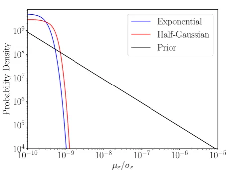
fore-ground for both ellipticity distributions are well within the background distribution, so we see no evidence for gravitational wave emission from the ensemble of pulsars. However, we can set upper limits on the ellipticity dis-tribution hyperparameters. Figure 8 shows the posteriors forµεand σεfor the exponential and half-Gaussian dis-tributions, respectively. From these we find 90% credible upper limits ofµ90%

ε ≤3.9×10−8andσ90%ε ≤4.7×10−8. These are about two orders of magnitude less constrain-ing than the purely spin-down limit based limits dis-cussed in Sec. II C, although they are the first such limits to be set based purely on gravitational wave observations.

VI. CONCLUSIONS

In this work we have described a Bayesian hierarchi-cal method for combining gravitational wave observa-tions from an ensemble of known pulsars for two pur-poses: to create a detection statistic for identifying a signal from the ensemble, and to estimate the parame-ters of the distribution of pulsars’ fiducial ellipticities.10

For two toy ellipticity distributions, an exponential and a half-Gaussian, we have used simulations to find that incorporating this distribution as a common prior on the ellipticity of stars, with an unknown hyperparameter, can produce a more efficient detection statistic than combin-ing the data for the ensemble of pulsars in a nonhierar-chical way. We also show that it is more efficient than a statistic derived in a similar way to that in [19]. We find that the detection of the ensemble could even be seen in cases where individual sources may not be individu-ally detectable with high confidence. However, we should note that the efficiency may not be improved if the true distribution does not well match our assumed prior form. For ensembles for which gravitational wave emission would be considered detected we have shown in Fig. 5 that we can correctly constrain the hyperparameters of the simulated ellipticity distribution. If no signal is seen we can also set upper limits on these. However, as shown in Fig. 6, we have also found that it is difficult to dis-tinguish between our two toy distributions as they are broadly similar.

10_{Here we have worked with fiducial ellipticities as they are a}

conve-nient and relatable quantity (i.e., they express the relative defor-mation of the star). However, the analysis actually estimates the mass quadrupole moment of the stars and converts that into the ellipticity given the canonical moment of inertia of 1038kg m2. So, one could convert back to the moment of inertia independent mass quadrupole if required. We should note that simulated sig-nals were drawn from the fiducial ellipticityεparameter, and we converted to mass quadrupoles using the canonical moment of inertia, so they do not incorporate a realistic equation-of-state dependent spread of moments of inertia.

We have performed the analyses using real data for 92 pulsars from the LIGO S6 science run, with the as-sumption of the same two ellipticity distributions: an exponential and a half-Gaussian. We saw no evidence of a signal from the ensemble, but set upper limits on the two distributions hyperparameters ofµ90%

ε ≤3.9×10−8 andσ90%

ε ≤4.7×10−

8_{. These upper limits are}

∼2 or-ders of magnitude less constraining than those that can be produced using the electromagnetically derived pulsar spin-down limits. However, they are the first such limits to be produced purely from gravitational wave observa-tions.

We note that the exponential and half-Gaussian dis-tributions used are rather simple. They were chosen as simple toy models that were easy to use due to being defined by a single hyperparameter. However, they are not necessarily physically realistic distributions. Obser-vationally, we know that there are different populations of pulsars, like the old recycled millisecond pulsars and the young pulsars. The fact that the former are most likely to have undergone an accretion phase, which could alter the structure of their crust and magnetic field strength com-pared to non-recycled pulsars, meaning they could well have a different distribution. So, it could be that the two populations should be treated independently, or a more complex distribution that allows separation of the two distributions should be used (for a simple case it could be a bimodal Gaussian).

It should also be noted that in this work we assume a 20% uncertainty of the distance to all pulsars, but in reality there are range of distance uncertainties from a few percent, or hundreds of percent. In a more thorough analysis the actual measurement uncertainties for each pulsar should be included, although we do not imagine it would lead to a particularly significant change in the results.

As discussed in Sec. II C the electromagnetic-observation-derived spin-down limits could be incorpo-rated more fully into the ellipticity distribution analysis. The simplest way to do this would be use the spin-down limits as a priors on the ellipticity (or mass quadrupole) for each pulsar. In this way, for pulsars for which the gravitational wave data alone is not particularly infor-mative the spin-down limit-based prior would dominate. Finally, it is worth highlighting that this type of anal-ysis would only constrain the underlying distribution of known pulsars, but not necessarily the entire neutron star population. There could, for example, be a different dis-tribution for accreting stars, or stars that are purely grav-itars (i.e. neutron stars that are purely spinning down due to gravitational wave emission.)

ACKNOWLEDGMENTS

Sci-10

₁₀

₁₀

₁₀

D

0

.

000

0

.

005

0

.

010

0

.

015

0

.

020

Ellipticity distribution

Exponential Foreground

Half-Gaussian Foreground

Background

Background

10

₁₀

₁₀

D

0

.

00

0

.

25

0

.

50

0

.

75

1

.

00

1

.

25

1

.

50

Non-hierarchical statistic

Foreground

Background

FIG. 7. The left panel shows the distributions ofDεexp_andDεhg _{for the foreground and background distributions from LIGO}

S6 data. The right panel showsDNH_{for the same data.}

10−10 ₁₀−9 ₁₀−8 ₁₀−7 ₁₀−6 ₁₀−5

Exponentialµε/Half-Gaussianσε 100

102 104 106 108

Probabilit

y

densit

y

Exponential Half-Gaussian Prior

FIG. 8. The posterior probability distributions for the hy-perparametersµε and σε defining the exponential and

half-Gaussian distributions respectively.

ence Foundation of China under Grants No. 11673008 and Newton International Fellowship Alumni Follow-on Funding. We are grateful for computational resources provided by Cardiff University, and funded by an STFC Grant No. (ST/I006285/1) supporting UK Involvement in the Operation of Advanced LIGO, and also those of the Atlas cluster at the Max-Planck Institut f¨ur Gravi-tationsphysik/Leibniz Universit¨at Hannover. We would like to thank members of the LIGO Scientific Collabo-ration and Virgo CollaboCollabo-ration, in particular members of the Continuous Waves (CW) working group, for use-ful discussions that have helped develop these ideas. We specifically thank Max Isi for his very useful comments

on draft versions of the paper. We would also like to thank the CW working group for the creation of the short Fourier transform data set of LIGO S6 data [48, 49] that we have used in this analysis. M.P. thanks the Institute for Nuclear Theory at the University of Washington, the Department of Energy, and the organizers and attendees of the “Astro-Solids, Dense Matter, and Gravitational Waves” workshop for their hospitality and for interesting discussion that enhanced this work.

This document has been given LIGO Document Num-ber ligo-p1800171 and INT preprint numNum-ber INT-PUB-18-037.

This work has been made possible thanks to a variety of software packages. The main analyses for each pulsar used software available in LALSuite [51]. The hierar-chical analysis used Python and functions written in Cython[52]. The post-processing was performed using Jupyter notebooks [53] and all plots have been produced usingMatplotlib[54, 55]. Pulsar data from the ATNF Pulsar Catalogue [16] has been accessed usingPSRQpy [56].

Appendix A:h0 posteriors

If an analysis produced posterior samples on the ob-served gravitational wave amplitude,h0, rather than on

εor Q22 (as has been the case for previous known

pul-sar searches), the analysis described in this paper could still be performed, although the marginalizations over the each pulsar’s distance would have to be explicitly computed. Assuming that a kernel density estimate has been used to turn sets ofh0posterior samples into

εi (assuming a uniform prior onh0 that is only nonzero

between zero and some maximumh0max) is

p(xi|εi, I) = Z Di

p(xi|h0=

κiεi

Di

, Di, I)

p(xi|I)

p(h0i|I)

dDi

= Z Di

p(h0i=

κiεi

Di |

xi, D, I)h0max×

p(xi|I)p(Di|I)dDi, (A1)

where

κi=

16π2_Gf rot2i

c4 Izz. (A2)

Appendix B: Evidence evaluation

Here we describe the various features/issues that we have found regarding evaluating the evidences. These relate to the systematic biases on evidences from nested sampling (see, e.g., [24]), and statistical uncertainties on the final evidence due to a combination of uncertainties from the KDE posterior estimates and statistical uncer-tainties on the individual pulsar evidences.

1. Statistical uncertainties on evidence values

To produce our final evidence values given by Eq. (9) we rely on the output of a code that uses a stochastic sampler to perform the required integrals. We also rely on a finite number of posterior samples from each pulsar’s estimate ofεto form a kernel density estimate of the true posterior. Both of these mean that even on identical initial data (with identical noise realizations) there will be some stochastic variation in the results.

To estimate these variations we have performed the processing described in Sec. III B 10 times on the same ensemble set, which in this case is one containing no pul-sar signals. A different random seed is used for the sam-pler in each case, otherwise the results really should be identical. To estimate the variations in the final evidence caused by the finite number of samples used for the KDE of theεposteriors, we use Eq. (16) but withp(xi|I) = 1 for each pulsar, so the only variation is from differences betweenp(εi|xi, I) in each analysis. We find that there is a standard deviation on the base-10 logarithm of the fi-nal evidence from Eq. (9) of_∼0.6, which comes from the variation in the estimates of the individual pulsarε pos-teriors. Each KDE is estimated using ∼1000 posterior samples, so we can check if this is roughly the variation you might expect. We can draw 1000 samples from 200 half-Gaussian distributions with known standard devia-tions, for each distribution produce a KDE and evalu-ate it at a range of points, sum the logarithms of these KDEs, and then numerically integrate it over the range of points. Doing this multiple times, but with the same set of standard deviations for each half-Gaussian, we find

the variation in the final integral is of the same order as that which we see for our analysis using simulated pul-sar data. This uncertainty can be reduced by increasing the number of posterior samples used for the KDE es-timate. To get more samples in our actual analysis we would need to use a greater number of nested sampling live points, which increases the run time. However, in fu-ture real analysis it may be worth doing this to cut down the uncertainties.

To see the uncertainty in the final evidence cause by both the stochastic variation in the individual pulsar ev-idencesand the KDE, we repeat the above with the ac-tual estimatedp(xi|I) for each pulsar. We find a stan-dard deviation on in the base-10 logarithm of the final evidence from Eq. (9) of_∼ 1.3. This suggests that the stochastic variations in the individual pulsar evidences and KDEs contribute roughly equally to the overall un-certainty. Again, this could be reduced by using a larger number of live points for the nested sampling algorithm. However, this variation is smaller than the distribution of background values, so will not be of great significance.

2. Systematic uncertainties on evidence values