Augmentation schemes for particle MCMC

Augmentation Schemes for Particle MCMC

Paul Fearnhead1∗, Loukia Meligkotsidou2.

1. Department of Mathematics and Statistics, Lancaster University. 2. Department of Mathematics, University of Athens.

* Correspondence should be addressed to Paul Fearnhead. (e-mail: [email protected]).

Abstract

Particle MCMC involves using a particle filter within an MCMC algorithm. For inference of a model which involves an unobserved stochastic process, the standard implementation uses the particle filter to propose new values for the stochastic process, and MCMC moves to propose new values for the parameters. We show how particle MCMC can be generalised beyond this. Our key idea is to introduce new latent variables. We then use the MCMC moves to update the latent variables, and the particle filter to propose new values for the parameters and stochastic process given the latent variables. A generic way of defining these latent variables is to model them as pseudo-observations of the parameters or of the stochastic process. By choosing the amount of information these latent variables have about the parameters and the stochastic process we can often improve the mixing of the particle MCMC algorithm by trading off the Monte Carlo error of the particle filter and the mixing of the MCMC moves. We show that using pseudo-observations within particle MCMC can improve its efficiency in certain scenarios: dealing with initialisation problems of the particle filter; speeding up the mixing of particle Gibbs when there is strong dependence between the parameters and the stochastic process; and enabling further MCMC steps to be used within the particle filter.

This is the author-accepted version. The final publication is available at link.springer.com

1

Introduction

Particle MCMC (Andrieu et al., 2010) is a recent extension of MCMC. It is most nat-urally applied to inference for models, such as state-space models, where there is an unobserved stochastic process. Standard MCMC algorithms, such as Gibbs samplers, can often struggle with such models due to strong dependence between the unobserved process and the parameters (see e.g. Pitt and Shephard, 1999; Fearnhead, 2011). Alter-native Monte Carlo methods, called particle filters, can be more efficient for inference about the unobserved process given known parameter values, but struggle when dealing with unknown parameters. The idea of particle MCMC is to embed a particle filter within an MCMC algorithm. The particle filter will then update the unobserved process given a specific value for the parameters, and MCMC moves will be used to update the parameter values. Particle MCMC has already been applied widely: in areas such as econometrics (Pitt et al., 2012), inference for epidemics (Rasmussen et al., 2011), and probabilistic programming (Wood et al., 2014). For recent results that demonstrate the good theoretical properties of particle MCMC see Chopin and Singh (2013) and Del Moralet al. (2014).

The standard implementation of particle MCMC is to use an MCMC move to update the parameters and a particle filter to update the unobserved stochastic process (though see Murray et al., 2012; Wood et al., 2014, for alternatives). However, this may be inefficient, due to a large Monte Carlo error in the particle filter, or due to slow mixing of the MCMC moves. The idea of this paper is to consider generalisations of this standard implementation, which can lead to more efficient particle MCMC algorithms.

In particular, we suggest a data augmentation approach, where we introduce new latent variables into the model. We then implement particle MCMC on the joint posterior distribution of the parameters, unobserved stochastic process and latent variables. We use MCMC to update the latent variables and a particle filter to update the parameters and the stochastic process. The intuition behind this approach is that the latent variables can be viewed as containing information about the parameters and the stochastic process. The more information they contain, the lower the Monte Carlo error of the particle filter. However, the more information they contain, the stronger the dependencies in the posterior distribution, and hence the poorer the MCMC moves will mix. Thus, by carefully choosing our latent variables, we are able to appropriately trade-off the error in the particle filter against the mixing of the MCMC, so as to improve the efficiency of the particle MCMC algorithm.

2014; Nemethet al., 2014). The re-parameterisation ideas presented in this paper could be employed together with many of these more advanced particle MCMC algorithms.

The ideas in this paper bear some similarity with the marginal augmentation approaches for improving the Gibbs sampler (e.g. van Dyk and Meng, 2001). In both cases, adding a latent variable to the model, and implementing the MCMC algorithm for this expanded model, can improve mixing. Our way of introducing the latent variables, and the way they are used are completely different though. However, both approaches can improve mixing for the same reason: introducing the latent variables reduces the correlation between variables updated at different stages of the Gibbs, or particle Gibbs, sampler.

In the next section we introduce particle filters and particle MCMC. Then in Section 3 we introduce our data augmentation approach. A key part of this is constructing a generic way of defining the latent variables so that the resulting particle MCMC algorithm is easy to implement. This we do by defining the latent variables to be observations of the parameters or of the stochastic process. By defining the likelihood for these observations to be conjugate to the prior for the parameters or the stochastic process we are able to analytically calculate quantities needed to implement the resultant particle MCMC algorithm. Furthermore, the accuracy of the pseudo-observations can be varied to allow them to contain more or less information. In Section 4 we investigate the efficiency of the new particle MCMC algorithms. We focus on three scenarios where we believe the data augmentation approach may be particularly useful. These are to improve the mixing of the particle Gibbs algorithm when there are strong dependencies between parameters and the unobserved stochastic process; to enable MCMC to be used within the particle filter; and to deal with diffuse initial distributions for the stochastic process. The paper ends with a discussion.

2

Particle MCMC

2.1 State-Space Models

For concreteness we consider application of particle MCMC to a state-space model, though both particle MCMC and the ideas we develop in this paper can be applied more generally. Throughout we will use p(·) and p(·|·) to denote general marginal and conditional probabililty density functions, with the arguments making it clear which distributions these relate to.

Our state-space model will be parameterised byθ, and we introduce a prior distribution for this parameter, p(θ). We then have a latent discrete-time Markov process, X1:T =

(X1, . . . , XT). We do not observe the state process directly. Instead we take partial

observations at each time-point,y1:T = (y1, . . . , yT). We assume that the observation at

is in calculating, or approximating, the posterior for the parameters and states:

p(x1:T, θ|y1:T) ∝ p(θ)p(x1:T|θ)p(y1:T|x1:T, θ)

= p(θ)

"

p(x1|θ)

T Y

t=2

p(xt|xt−1, θ)

# " _T Y

t=1

p(yt|xt, θ) #

. (1)

We frequently use the notation of an extended state vectorX_t= (x1:t, θ), which consists

of the full path of the state process to timet, and the value of the parameter. ThusXT

consists of the full state-process and the parameter, and we are interested in calculating or approximatingp(X_T|y1:T).

2.2 Particle Filters

Particle filters are Monte Carlo algorithms that can be used to approximate posterior distributions for state-space models, such as (1). For reasons that will be apparent later, we will consider the generalisation where we condition on Z, a function of X_T. Thus the particle filter will target p(XT|Z, y1:T) = p(x1:T, θ|Z, y1:T). A simple particle filter

algorithm is given in Algorithm 1.

Algorithm 1 Particle Filter Algorithm Input:

A value of Z.

The number of particle,N.

1: fori= 1, . . . , N do

2: SampleX₁(i) independently fromp(X1|Z).

3: Calculate weightsw(₁i)=p(y1|X1(i),Z).

4: end for

5: Set ˆp(y1|Z) = _N1 PNi=1w (i) 1 .

6: fort= 2, . . . , T do

7: fori= 1, . . . , N do

8: Sample j from {1, . . . , N} with probabilities proportional to{w_t(1)₋₁, . . . , w(_t−N₁)}.

9: Sample X_t(i) from p(Xt|Xt(−j)1,Z).

10: Calculate weightsw_t(i)=p(yt|Xt(i),Z). 11: end for

12: Set ˆp(y1:t|Z) = ˆp(y1:t−1|Z)

1

N

PN

i=1w

(i)

t

.

13: end for

14: Samplej from {1, . . . , N}with probabilities proportional to{w_T(1), . . . , w(_TN)}

Output: A value of the extended state,X_T(j), and an estimate of the marginal likelihood ˆ

If we stopped this particle filter algorithm at the end of iterationt, we would have a set of values for the extended state, often called particles, each with an associated weight. These weighted particles give an approximation to p(X_t|y1:t,Z). At iteration t+ 1 we

propagate the particles and use importance sampling to create a set of weighted particles to approximate p(Xt+1|y1:t+1,Z). This involves first generating new particles at time t+ 1 through (i) sampling particles from the approximation to p(X_t|y1:t,Z); and (ii)

propagating these particles by simulating values for Xt+1 from the transition density of the state-process, p(Xt+1|Xt,Z). Secondly, each of these particles att+ 1 is then given

a weight proportional to the likelihood of the observation yt+1 for that particle value. See Doucetet al. (2000) and Fearnhead (2008) for more details. At the end of iteration T we can output a single value of XT, by sampling once from the particles at time T,

with the probability of choosing a particle being proportional to its weight.

A by product of the importance sampling at iterationt+ 1 is that we get a Monte Carlo estimate of p(yt+1|y1:t,Z), and the product of these for t = 1, . . . , T gives an unbiased

estimate of the marginal likelihoodp(y1:T|Z) (Del Moral, 2004, proposition 7.4.1). This

unbiased estimate will be key to the implementation of particle MCMC.

2.3 Particle MCMC

The idea of particle MCMC is to use a particle filter within an MCMC algorithm. There are two generic implementations of particle MCMC: particle marginal Metropolis-Hastings (PMMH) and particle Gibbs.

Particle marginal Metropolis-Hastings Algorithm

First we describe the particle marginal Metropolis-Hastings (PMMH) sampler (Andrieu

et al., 2010, Section 2.4.2). This involves choosing Z, an appropriate function of the extended state, X_T. Our MCMC algorithm has a state that is {Z,X_T,pˆ(y1:T|Z)}, a

value for this function, a corresponding value for the extended state and an estimate for the marginal likelihood given the current value ofZ. We assume thatZ has been chosen so that we can both implement the particle filter of Algorithm 1, and also that we can calculate the marginal distribution,p(Z). A common choice isZ =θ, though see below for other possibilities.

Within each iteration of PMMH we first propose a new value for Z, using a random walk proposal. Then we run a particle filter to both propose a new value of XT and to

calculate an estimate for the marginal likelihood. These new values are then accepted with a probability that depends on the ratio of the new and old estimates of the marginal likelihood. Full details are given in Algorithm 2.

Algorithm 2 Particle marginal Metropolis-Hastings Algorithm (Andrieuet al., 2010) Input:

An initial valueZ(0)_.

A proposal distributionq(·|·).

The number of particles,N, and the number of MCMC iterations, M.

1: Run Algorithm 1 with N particles, conditioning on Z(0)_{, to obtain X}(0)

T and

ˆ

p(y1:T|Z(0)).

2: fori= 1, . . . , M do

3: SampleZ0 _{from q(Z|Z}(i−1)_).

4: Run Algorithm 1 with N particles, conditioning on Z0, to obtain X_T0 and ˆ

p(y1:T|Z0). 5: With probability

min

(

1, q(Z

(i−1)_|Z0_)ˆp(y

1:T|Z0)p(Z0)

q(Z0_|Z(i−1)_)ˆp(y

1:T|Z(i−1))p(Z(i−1)) )

set X_T(i) = X_T0, Z(i) _{= Z}0 _{and ˆp(y}

1:T|Z(i)) = ˆp(y1:T|Z0); otherwise set X_T(i) =

X_T(i−1),Z(i)_=Z(i−1) _{and ˆp(y}

1:T|Z(i)) = ˆp(y1:T|Z(i−1)) 6: end for

Output: A sample of extended state vectors: {X_T(i)}M i=1.

MCMC algorithm. If we ignore the approximation, and denote the current state by (X_T,Z), then the acceptance probability of this MCMC algorithm would be

min

1,q(Z|Z

0_)p(y

1:T|Z0)p(Z0)

q(Z0_|Z)p(y

1:T|Z)p(Z)

,

as the p(X_T0|Z0) terms cancel as they appear in both the target and the proposal. The actual acceptance probability we use just replaces the, unknown, marginal likelihoods with our estimates. The magic of particle MCMC is that despite these two approxima-tions, both in the proposal distribution forXT given Z and in the marginal likelihoods,

the resulting MCMC algorithm has the correct stationary distribution.

Particle Gibbs

The alternative particle MCMC algorithm, particle Gibbs, aims to approximate a Gibbs sampler. A Gibbs sampler that targetsp(Z,XT|y1:T) would involve iterating between (i)

sampling a new value for Z from its full-conditional given the other components of X_T; and (ii) sampling a new value for XT from its full conditional givenZ,p(X1:T|Z, y1:T).

be calculated analytically.

The difficulty, however, comes with implementing step (ii). The idea of particle Gibbs is to use a particle filter to approximate this step. Denote the current value forX1:T by

X_1:∗_T. Then, informally, this involves implementing a particle filter but conditioned on one of the particles at timeT beingX∗

1:T. We then sample one of the particles at timeT

from this conditioned particle filter and updateX1:T to the value of this particle. This

simulation step is called a conditional particle filter, or a conditional SMC sampler. For full details of this see Andrieu et al. (2010).

2.3.1 Implementation

Whilst both particle MCMC algorithms have the correct stationary distribution regard-less of the accuracy of the particle filter, the accuracy does affect the mixing properties. More accurate estimates of the marginal likelihood will lead to more efficient algorithms (Andrieu and Roberts, 2009). In implementing particle MCMC, as well as choosing de-tails of the proposal distribution for Z, we need also to choose the number of particles to use in the particle filter. Theory guiding these choices for PMMH is given in Pitt

et al. (2012), Doucetet al. (2012) and Sherlock et al. (2015).

The standard implementation of particle MCMC will have Z = θ. However, our de-scription is aimed to stress that particle MCMC is more general than this. It involves using MCMC proposals to update part of the extended state, and then a particle filter to update the rest. There is flexibility in choosing which part is updated by the MCMC move and which by the particle filter within the particle MCMC algorithm. For exam-ple, in order to deal with a diffuse initial distribution for the state-process, Murrayet al.

(2012) choose Z = (θ, X1), so that MCMC is used to update both the parameters and the initial value of the state-process. Alternatively, Woodet al.(2014) chooseZ=∅, so that both the parameters and the path of the state are updated using the particle filter.

To demonstrate this flexibility, and discuss its impact on the performance of the particle MCMC algorithm, we will consider a simple example.

2.4 Example of Particle MCMC for linear-Gaussian Model

We consider investigating the efficiency of particle MCMC for a simple linear-Gaussian model where we can calculate the posterior exactly. The model has a one-dimensional state process, defined by

1 10 100 1000 10000

0

10

20

30

40

50

(a)

Sigma_1

A

CT

1e−02 1e−01 1e+00 1e+01 1e+02

0

10

20

30

40

50

(b)

k_Z

A

CT

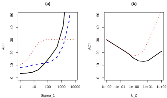
Figure 1: Autocorrelation Times (ACT) for Particle MCMC runs of the Linear-Gaussian Model. (a) ACT for three particle MCMC algorithms as we vary σ1: Z = ∅ (black),

Z = {θ} (blue dashed), Z = {θ, X1} (red dotted). (b) ACT for particle MCMC with pseudo-observations,Z = (Zx, Zθ) as we vary the variance of the noise in the definition

of pseudo-observations; the variance of the noise forZx andZθ iskZ times the marginal

posterior variance forX1 and θrespectively. ACT is shown forX1 (black) andZx (red

dotted).

where(_tX)are independent standard normal random variables. Fort= 1, . . . , T we have observations

Yt=θ+Xt+σY(tY),

where(_tY) are independent standard normal random variables. We assume thatσ2 1,σX2,

σ_Y2 and γ are known, and thus the only unknown parameter is θ. Finally, we assume a normal prior for θwith mean 0 and variance σ_θ2.

We simulated data for 100 times steps, withγ = 0.99, σY = 20 andσX chosen so that

that Xt process will have variance of 1 at stationarity. Our interest was in seeing how

particle MCMC performs in situations where there is substantial uncertainty inX1 and θ. Here we present results with σθ = 100 as we vary σ1. We implemented particle MCMC with Z =∅,Z ={θ} and Z ={θ, X1}. For the latter two implementations we used a random walk update forθandX1with the variance set to the posterior variance; with independent random walk updates for θand X1 when Z ={θ, X1}.

To evalulate performance we ran each particle MCMC algorithm using 100 particles and 250,000 iterations. We removed the first quarter of iterations as burn-in, and calculated autocorrelation times for estimatingθ. These are shown in Figure 1(a).

to smaller proposed moves, with the proposed new values for θ and/or X1 depending on their current values. However, more information in Z, comes at the advantage of smaller Monte Carlo error in the estimate of the likelihood from the particle filter. This reduction in Monte Carlo error becomes increasingly important as the prior variance for X1 increases. So for smaller values ofσ1 the best algorithm hasZ =∅, whereas when we increase σ1 first the choice ofZ ={θ} then the choice of Z={θ, X1} performs better.

3

Augmentation Schemes for Particle MCMC

The example at the end of the previous section shows that the choice of which part of the extended state is updated by the particle filter, and which by a standard MCMC move, can have a sizeable impact on the performance of particle MCMC. Furthermore the default option for state-space models of updating parameters by MCMC and the state-process by a particle filter, is not always optimal.

The potential within this choice can be greatly enhanced by augmenting the original model. We will introduce an extra latent variable, Z, drawn from some distribution conditional onXT. This will introduce a new posterior distribution

p(XT, z|y1:T) =p(XT|y1:T)p(z|XT), (2)

wherep(X_T|y1:T) is defined by (1) as before.

For any choice of p(z|XT), if we marginalise Z out of (2) we get (1). Our approach

will be to implement a particle MCMC algorithm for sampling from (2). This will give us samples {X_T(i), z(i)_}M

i=1 from (2), with the {X (i)

T }Mi=1 from (1) as required. In implementing the particle MCMC algorithm, we will chooseZ =z. That is, we update the latent variable,Z, using the MCMC move, and we use a particle filter to updateX_T

conditional onZ and y1:T.

Whilst, in theory, we have a completely free choice over the distribution of the new latent variable, Z, in practice we need to be able to easily implement the resulting particle MCMC algorithm. In practice this will mean that we need to be able to easily simulate fromp(θ|z),p(x1|z, θ) and, for t= 2, . . . , T,p(xt|Xt−1, z). For PMMH we will also need to be able to calculate the acceptance probability of the algorithm, which involves the term

p(z) =

Z

p(z|X_T)p(X_T)dX_T =

Z

p(z|θ, x1:T)p(θ)p(x1)

T Y

t=2

p(xt|xt−1)dθdx1:T.

3.1 Generic Augmentation Schemes: Pseudo-Observations

In choosing an appropriate latent variable Z we need to first consider the ease with which we can implement the resulting particle MCMC algorithm. A generic approach is to model Z as an observation of either θ orx1 or both. As Z is a latent variable we have added to the model, we call these pseudo-observations.

By the Markov property of the state-process, if Z only depends onθand/or x1 then we havep(xt|Xt−1, z) =p(xt|Xt−1). Thus to be able to implement the particle filters we only

need to choose our model for the pseudo-observation so that we can simulate fromp(θ|z) andp(x1|z, θ). To enable this we can let each component ofZbe an independent pseudo-observation of a component of θ or x1, with the likelihood for the pseudo-observation chosen so that the prior for the relevant component of θ or x1 is conjugate to this likelihood. Conjugacy will ensure that not only can we simulate from the necessary conditional distributions but we can also calculate p(z) as required to implement the particle MCMC algorithms. Constructing such models for the pseudo-observations is possible for many state-space models of interest. In some applications other choices for Z may be necessary or advisable: see Section 4.2 for an example.

To make these ideas concrete consider the linear Gaussian model of Section 2.4. We can choose Z = (Zθ, Zx) whereZθ is a pseudo-observation ofθ and Zx is one of X1. As we

have both a Gaussian prior forθand a Gaussian initial distribution forX1, in each case a conjugate likelihood model arise from observations with additive Gaussian error. So for example we could choose

Zθ|θ∼N(θ, τ2). (3)

This would give a marginal distribution ofZθ ∼N(0, τ2+σθ2) and a conditional

distri-bution of

θ|zθ∼N

zθσθ2

τ2_+σ2

θ

, τ 2_σ2

θ

τ2_+σ2

θ !

.

Consider the case where we letZ depend only on θ. In specifyingp(z|θ) we will have a choice as to how informativeZis aboutθ– for example the choice ofτ in (3) for the linear Gaussian model example. As such this gives a continuum between the implementations of particle MCMC in Section 2.3. In the limit asZ is increasingly informative aboutθ, we converge on an implementation of particle MCMC where we updateθ using MCMC and X1:T using the particle filter. As Z becomes less informative, we would tend to

an implementation of particle MCMC where both θand X1:T are updated through the

particle filter.

To gain some intuition about the effect of the choice of Z we implemented particle MCMC for the linear-Gaussian model withZ = (Zx, Zθ) chosen as above. We simulated

data as described in Section 2.4, but with σ1 =σθ = 1,000. Our aim is to investigate

of the noise in the definition ofZx andZθ. For this model we can calculate analytically

the true posterior distribution for X1 and θ, and we chose the variance of the pseudo observations to be proportional to the marginal posterior variances. So for a chosenkZ

we set

Var(Zx|x1) =kZVar(X1|y1:100), and Var(Zθ|θ) =kZVar(θ|y1:100).

Figure 1 (b) shows the resulting auto-correlation times for X1 and ZX as we vary kZ.

Choosing kZ ≈ 0 gives auto-correlation times similar to running particle MCMC with

Z ={X1, θ}. As kZ is increased the efficiency of the particle MCMC algorithm initially

increases. The intuition is that there is an underlying ideal MCMC algorithm linked to particle MCMC, which is the MCMC algorithm we obtain if the SMC estimate of the marginal likelihood were exact. As kZ increases we expect better mixing of this

underlying MCMC algorithm as we are conditioning on less information (see also Section 3.2). However for very large kZ values the efficiency of particle MCMC becomes poor.

In this case it starts behaving like particle MCMC with Z = ∅, for which the large Monte Carlo error in estimating the likelihood leads to poorer mixing. The best values of kZ correspond to adding noise to the pseudo-observations which is similar in size to

the marginal posterior variances of X1 and θ, and we notice good performance for a relatively large range of kZ values.

3.2 Pseudo Observations for Particle Gibbs

We can gain some understanding of the benefit of using pseudo observations within particle Gibbs, by considering the mixing properties of the idealised Gibbs sampler that particle Gibbs is approximating. Assume we introduce pseudo observations, Z, of the parameters. Particle Gibbs approximates a Gibbs sampler where we iterate between updating Z given XT = (x1:T, θ) and XT given Z. Andrieu et al.(2013) give results on

the mixing of a Particle Gibbs algorithm in terms of the mixing of the underlying Gibbs sampler. Under certain regularity conditions, they show that spectral gap of a particle Gibbs algorithm is bounded by a constant times the spectral gap of the idealised Gibbs sampler it approximates. Furthermore, as the number of particles increases the lower bound on the spectral gap of particle Gibbs converges to the spectral gap of the idealised Gibbs sampler.

We can interpret these results informally, as saying that, if we use sufficiently many particles, we expect the mixing of particle Gibbs will be similar to that of the idealised Gibbs sampler. Standard results for the Gibbs sampler give the following results for the mixing of this idealised sampler.

Theorem 1. Assume we have a Gibbs sampler that targets a joint distribution for

(Z,XT), where XT = (θ, x1:T), and which iterates between updates of Z given XT and

(i) If Z is conditionally independent of x1:T given θ, anda is a vector, then the lag-1

correlation for aTZ is

aTvar(Z)a−aTE[var(Z|θ)]a aT_var(Z)a ,

(ii) If E(Z|θ) = θ, and there exists a λ >0 such that Var(Z|θ)−λVar(θ) is positive definite, then the lag-1 correlation of aTZ is bounded above by 1/(1 +λ).

(iii) Finally, if Z =θ+where is an independent copy of θ then the geometric rate of convergence of the algorithm is bounded above by 1/√2.

Proof. For part (i) we use the result that from Liu et al. (1994) (see also Amit, 1991; Liu, 1994) that the lag-1 autocorrelation of aTZ, for some fixed vectora is

1−a

T_{E [var(Z|X}

T)]a

aT_var(Z)a .

Now as var(Z) = var(E(Z|θ)) + E(var(Z|θ)) we can re-write the result in (i) to give that the lag-1 correlation foraTZ is

aTvar(E(Z|θ))a

aT_{var(E(Z|θ))a+a}T_{E(var(Z|θ))a}.

For part (ii), we have E(Z|θ) =θ. So the lag-1 autocorrelation is

aTvar(θ)a

aT_var(θ)a+aT_{E(var(Z|θ))a}.

This is a decreasing function ofaTE(var(Z|θ))a. By the condition on var(Z|θ), we have thataT_{E(var(Z|θ))> λa}T_{var(θ)a, which gives the required bound.}

Finally part (iii) uses the fact that the geometric rate of convergence is the maximal correlation between XT and Z (Liu et al., 1994). The maximal correlation can then be

bounded using standard results for the maximal correlation of partial sums of indepen-dent and inindepen-dentically distributed random variables (Demboet al., 2001).

θ and x1:T, where the idealised Gibbs sampler relating to the standard particle Gibbs

algorithm will mix very slowly. In such cases we would expect that the improvement in mixing of the idealised Gibbs sampler that we obtain by adding noise which is, say, similar in distribution to the posterior for θ will more than compensate the need for more particles to control the Monte Carlo variability of the conditional SMC sampler. Parts (ii) and (iii) also suggest that if we have Z such that E(Z|θ) =θ, then we should choose the variance of Z to be of the order of the posterior variance of θ.

3.3 MCMC within PMCMC

One approach to improve the performance of a particle filter is to use MCMC moves within it (see Gilks and Berzuini, 2001). An example is to use a MCMC kernel to update particles prior to propagating them to the next time-step. This involves a simple adapta-tion of Algorithm 1. Assume thatKt−1(·|·) is a Markov kernel that hasp(Xt−1|y1:t−1,Z) as its stationary distribution. Then we change step 9 of Algorithm 1 to:

9: SampleX∗

t−1 fromKt−1(·|Xt(−j)1), andX (i)

t from p(Xt|Xt∗−1,Z).

The use of such an MCMC step can be particularly helpful for updating parameters, as they help to ensure some diversity in the set of parameter values stored by the particles is maintained, and, as a consequence, can improve the accuracy of estimates of the marginal likelihood. Where possible, a common choice of kernel is to update just the parameters of the particle by sampling from the full conditional p(θ|x1:t−1, y1:t−1).

Often such updates can be implemented in a computationally efficient manner as the full conditional distribution just depends on the state-path through fixed-dimensional sufficient statistics (Storvik, 2002; Fearnhead, 2002). For recent examples of the benefits of using such MCMC moves see, for example, Carvalho et al. (2010a), Carvalho et al.

(2010b) and Gramacy and Polson (2011).

4

Examples

4.1 Stochastic Volatility

A simple stochastic volatility model assumes a univariate state-process, defined as

X1=σ0(1X); andXt=γXt−1+σX(tX), fort= 2, . . . , T ,

where(_tX)are independent standard normal random variables. Fort= 1, . . . , T we have observations

Yt=σY exp{xt}(tY),

where (_tY) are independent standard normal random variables. Thus the state pro-cess governs the variance of the observations, with larger values of xt meaning larger

variability in the observation at timet.

We assume θ = (γ, σX, σY) are unknown. We introduce independent priors, with γ

having a normal distribution with mean µγ and variance σγ2, but truncated to (−1,1);

whileβX = 1/σX2 andβY = 1/σ2Y have gamma prior distributions with shape parameters

aX and aY respectively, and scale parameter bX and bY respectively. We assume that

σ0 = 1.

We introduce a four-dimensional pseudo-observationZ = (ZX, Zγ, ZβX, ZβY) where

con-ditional on (X1, γ, βX, βY)

ZX ∼N(X1, τX2), Zγ ∼N(γ, τγ2),

ZβX ∼gamma(nX, βX),andZβY ∼gamma(nY, βY).

This choice for the pseudo-observations ensures that we can calculate the required marginal and conditional distributions, see Appendix A for details. To finalise the spec-ification of these models we need to choose the values for τX, τγ, nX and nY which

determine how informative the pseudo-observations are.

Particle Gibbs

We first compare different implementations of the Particle Gibbs algorithm. Our focus here is to show that using pseudo-observations can improve mixing in scenarios where the idealised Gibbs sampler would mix poorly. This corresponds to situations where there is strong dependence in the state-process.

We simulated data with T = 1,000 observations, γ = 0.99, σY = 1 and σX = 1/(1−

0.992), so that the stationary variance of the state process is 1. We present results for priors withµγ = 0.5 andσ2γ= 0.5;aX = 1 andbX = 1/1000; andaY = 0.1 andbY = 0.1.

This corresponds to the true values of γ and βX being in the tails of the prior, and a

We implemented both the standard version of Particle Gibbs, with Z=θ, and Particle Gibbs with conditioning on the pseudo-observations, Z = Z defined above. Note that there exists a constant C such that E[log(ZβX −C)] = log(βX), and var[log(ZβX)] is a

constant that depends onnX; and similarly forZβY. Thus Theorem 1 suggest we choose

τX,τγ,nX and nY so that the conditional variances ofZX,Zγ, log(ZβX) and log(ZβY)

are similar to the posterior variances for X1, γ, log(βX) and log(βY) respectively. We

chose these tuning parameters so that the conditional variances were slightly smaller than the posterior variances we observed from a pilot run. For further comparison we show results for Particle Gibbs with no conditioning, Z = ∅, again implemented with N = 500.

We ran the standard version with N = 250 particles, and the other two versions with N = 500. This was based on choosing N so that the estimate of the log-likelihood had a variance of around 1 (Pitt et al., 2012). To compensate for the doubling of the computational cost of the conditional SMC sampler with the latter two versions, we ran the standard version of the Particle Gibbs for twice as many iterations. To ease comparison of results we then thinned the output by keeping the values of the chain on even iterations only.

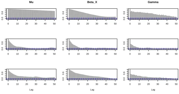
Results are shown in Figure 2. The standard implementation performs badly here. This is because of strong dependencies between the parameters and the state-process that occurs for this model which means that the underlying Gibbs sampler mixes slowly. By conditioning on less information when running the conditional SMC sampler we reduce this dependence between the X_T and Z which improves mixing. However, choosing

Z = ∅ results in a substantial decrease in efficiency of the conditional SMC sampler. This is particularly pronounced due to the relatively uninformative priors we chose, and the fact that one of the parameter values was in the tail of the prior. If much more informative priors were chosen, using Z = ∅ would give similar results to the use of pseudo-observations. Also this effect could be reduced slightly by increasing N further for this implementation of Particle Gibbs, but doing so will still lead to a less efficient sampler than using pseudo-observations.

PMMH with MCMC

We now compare PMMH on the stochastic volatility model. Our focus is purely on how using MCMC within the particle filter can help improve mixing over a standard PMMH algorithm. We simulated data with parameter values as above. To help reduce the computational cost involved in analysing this data, and hence implementing the simulation study, using PMMH we use more informative priors (which meant we could use fewer particles when running the particle filters), withµγ= 0.9 andσγ2 = 0.1;aX = 1

and bX = 1/100; andaY = 1 andbY = 1.

0 10 20 30 40 50 0.0 0.6 A CF Mu

0 10 20 30 40 50

0.0

0.6

Beta_X

0 10 20 30 40 50

0.0

0.6

Gamma

0 10 20 30 40 50

0.0

0.6

A

CF

0 10 20 30 40 50

0.0

0.6

0 10 20 30 40 50

0.0

0.6

0 10 20 30 40 50

0.0

0.6

Lag

A

CF

0 10 20 30 40 50

0.0

0.6

Lag

0 10 20 30 40 50

0.0

0.6

Lag

Figure 2: ACF plots for three runs of the Particle Gibbs conditioning on: Z = θ (top row);Z =Z (middle row); andZ =∅(bottom row). Each column corresponds to ACF for a different parameter: µ= log(βY) (left column); βX (middle column); and γ (right

column).

values, using standard Particle Learning algorithms (Carvalho et al., 2010a). Using the criteria of Pitt et al. (2012), we choseN = 150 and N = 450 particles respectively for these implementations. We used random walk proposals with the variances informed by a pilot run (Roberts and Rosenthal, 2001). Again we compensate for the slow running of the PMMH with pseudo-observations by running the other PMMH algorithm for three times as long, and thinning: keeping only every third value.

The main improvement in efficiency we observed with the second PMMH algorithm was through using the diversity in parameter values we obtain when using the Particle Learning Algorithm. Our approach for implementing this was to output a set of equally weighted particle values from the particle learning algorithm. We then make a decision as to whether to accept this set of particles, with the normal acceptance probability. Finally, we add an extra step to each iteration where we resample the state of the PMMH algorithm from the last stored set of particles. Full details are given in Algorithm 3 in Appendix B.

Mu

Iteration 0 1000 2000 3000 4000

−0.6 −0.2 0.2 0.6 Beta_X Iteration 0 1000 2000 3000 4000

20 60 100 140 Gamma Iteration 0 1000 2000 3000 4000

0.95

0.97

0.99

Mu

Iteration 0 1000 2000 3000 4000

−1.0

0.0

0.5

Beta_X

Iteration 0 1000 2000 3000 4000

20 60 100 140 Gamma Iteration 0 1000 2000 3000 4000

0.95

0.97

0.99

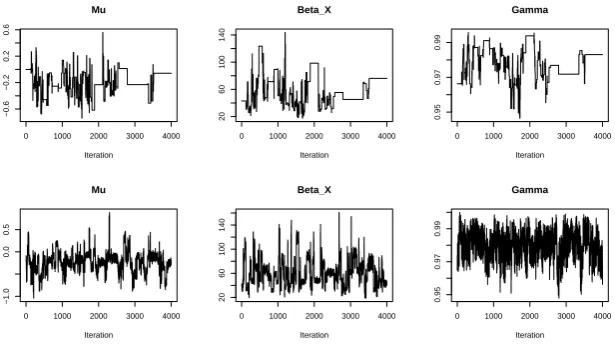
Figure 3: Trace plots for two runs of PMMH: Z = θ (top row); and Z = Z (bottom row). Each column corresponds to a different parameter: µ= log(βY) (left column); βX

(middle column); andγ (right column).

and γ. Note that we can use particle learning with particle MCMC if we chooseZ =∅. The effectiveness of the resulting particle MCMC algorithm will depend crucially on how informative the priors are, and the degree of similarity between the prior and posterior. For uninformative priors, or priors which place little mass in areas of high posterior probability, using Z = ∅ will be inefficient due to a large increase in the Monte Carlo error of the particle filter.

4.2 Dirichlet Process Mixture Models

We now consider inference for a mixture model used to infer population structure from population genetic data. Assume we have data from a set of diploid individuals, and this data consists of the genotype of each individual at a set of unlinked loci. Thus each locus will have a set of possible alleles (different genetic types), and the data for an individual at that locus will be which alleles are present on each of two copies of that individual’s genome. We further assume that the individuals each come from one of an unknown number of populations. The frequency of each allele at each locus will vary across these populations. We wish to infer how many populations there are, and which individuals come from the same population.

This is an important problem in population genetics. We will consider a model based on that of Pritchard et al. (2000a). Though see Pritchard et al. (2000a), and Falush

et al. (2003) for extensions of this model; Pritchard et al. (2000b) and Rosenberget al.

alternative approaches to this problem.

Assume we haveLloci. At locuslwe haveKlalleles. The allele frequencies of these

alle-les in populationjare given byp(j,l)= (p₁(j,l), . . . , p(_Kj,l)

l ). The genotype of individualiat

locuslisyi,l= (y(1)_i,l, y(2)_i,l). Letxi be a unobserved latent variable which defines the

pop-ulation that individualiis from. Then the conditional likelihood ofyi = (yi,1, . . . ,yi,L)

given xi =j is

p(yi|xi=j) = L Y

l=1 p(j,l)

y(1)_i,l p

(j,l)

y_i,l(2).

This model assumes the loci are unlinked and there is no admixture, hence conditional on xi the data at each locus are independent.

We assume conjugate Dirichlet priors for the allele frequencies in each population. These priors are independent across both loci and population. For locuslthe parameter vector of the Dirichlet prior is (λ/Kl, . . . , λ/Kl).

We use a mixture Dirichlet process (MDP) model (Ferguson, 1973) for the prior distri-bution of latent variables xi. We will use the following recursive representation of the

MDP model (Blackwell and MacQueen, 1973). Letx1:i= (x1, . . . , xi) be the population

of origin of the first i individuals, and define m(x1:i) to be the number of populations

present in x1:i. We number these populations 1, . . . , m(x1:i), and let nj(x1:i) be the

number of these individuals assigned to populationj. Then

p(xi+1 =j|x1:i) = (

nj(x1:i)/(i+α) ifj≤m(x1:i),

α/(i+α) ifj=m(x1:i) + 1.

(4)

This model does not pre-specify the number of populations present in the data. Note that the actual labelling of populations under the MDP model is arbitrary, and the infor-mation inx1:nis essentially which subset of individuals belong to each of the populations.

In our implementation the actual labels are defined by the order of the individuals in the data set. With population 1 being the population that the first individual belongs to, population 2 is the population that the first individual not in population 1 belongs to, and so on.

Inference for this model was considered in Fearnhead (2008) for the case whereλandα were known. Here we introduce hyperpriors for both these parameters, and perform infer-ence using particle MCMC. We use independent gamma priors, withα∼Gamma(5,10) and λ ∼ Gamma(4,1). If we condition on values for λ and α, then Fearnhead (2008) presents an efficient particle algorithm for this problem. This particle filter is based on ideas in Fearnhead and Clifford (2003) and Fearnhead (2004).

0 20 40 60 80

0.0

0.2

0.4

0.6

0.8

1.0

(a)

i

Probability

0 20 40 60 80

−300

−100

0

100

(b)

i

Logit(Probability)

Figure 4: Plot of (a) Pr(X1 =X2|y1:i) and (b) logit[Pr(X1 =X2|y1:i)] for different sizes

of data seti.

Figure 4 plots estimates of Pr(X1 =X2|y1:i) for increasing values of i. This shows how

the posterior probability of the first two individuals being from the same population changes as we analyse data from more people. Initially this is close to 1, whereas once all data has been analysed the probability is essentially 0. This substantial change in probability causes problems in a particle filter, as all particles withx1 6=x2 are likely to lost during resampling in the early iterations of the algorithm.

To overcome this problem of initialisation of the particle filter for this application we pro-pose to introduce a pseudo observation,Zx, that contains information about the

popula-tions of a random subset of the individuals. The distribution ofZx givenx1:nis obtained

by (i) sampling the number of individuals in the subset,vsay; (ii) choosingvindividuals at random from the sample,i1, . . . , iv; and (iii) lettingZx={(i1, xi1), . . . ,(iv, xiv)}, the

subset of individuals and their population labels.

As mentioned above, the actual values of the population labels is arbitrary, and Zx

just contains information about which of the individuals i1, . . . , iv belong to the same

population. In practice, at each iteration we re-order the individuals in the sample so that individualsi1, . . . , iv become the first vindividuals, and the order of the remaining

individuals is chosen uniformly at random. The labels for the new firstvindividuals are changed to be consistent with our recursive represenation of the MDP model above.

In implementing PMCMC we use Z = (λ, α, Zx). Our proposal distribution for Zx is

just its true conditional distribution given x1:n. We can easily adapt the particle filter

0 2000 4000 6000 8000 1.7 1.8 1.9 2.0 2.1 2.2 Repar. PMCMC Iteration A CF

0 2000 4000 6000 8000

1.7 1.8 1.9 2.0 2.1 2.2 PMCMC N=20 Iteration

0 2000 4000 6000 8000

1.7 1.8 1.9 2.0 2.1 PMCMC N=40 Iteration

0 2000 4000 6000 8000

1.7 1.8 1.9 2.0 2.1 2.2 PMCMC N=60 Iteration

0 10 20 30 40

0.0 0.2 0.4 0.6 0.8 1.0 Lag Lambda

0 10 20 30 40

0.0 0.2 0.4 0.6 0.8 1.0 Lag

0 10 20 30 40

0.0 0.2 0.4 0.6 0.8 1.0 Lag

0 10 20 30 40

0.0 0.2 0.4 0.6 0.8 1.0 Lag

Figure 5: Trace plots (top) and acf plots (bottom) forλfor the reparameterised PMCMC with Z = (λ, α, Zx) (left-hand column), and standard PMCMC with Z = (λ, α) (other

columns). We ran the reparameterised PMCMC withN = 20 particles, and the standard PMCMC withN = 20,N = 40 andN = 60 particles. Results shown after removing the first 105 iterations as burn-in and thinning the remaining output by keeping only every 100th value.

the sample to those specified byZx. We use a random walk proposal for updating logλ

and an independence proposal forα. Further details are given in Appendix C.

We compared the reparameterised PMCMC with this choice of Z with a standard PM-CMC algorithm whereZ = (λ, α). Our aim is purely to investigate the relative efficiency of the two implementations of PMCMC on this challenging problem. We ran each PM-CMC algorithm for 106 _{iterations, storing only every 100th value. We implemented the} new PMCMC algorithm using 20 particles for the particle filter, and with Zx storing

We see that the reparameterised PMCMC algorithm has substantially better mixing than the standard PMCMC algorithm, even when the latter used 3 times as many particles, and hence would have three times the CPU cost per iteration. For all the standard PMCMC algorithms, the chain gets stuck for substantial periods of time. This is due to a large variance of the estimate of the likelihood. By running the particle filter conditional on Zx we obtain a substantial reduction in the variance of our estimates of

the likelihood, and hence avoid this problem.

Estimated auto-correlation times are 1.3 for the reparameterised PMCMC algorithm with 20 particles, and 105, 56 and 36 for the standard PMCMC with 20, 40 and 60 particles respectively. After taking account that the CPU cost of an iteration of PMCMC is proportional to the number of particles, this suggests the re-parameterised PMCMC is about 80 times more efficient than each of the standard PMCMC algorithms.

5

Discussion

We have introduced a way to generalise particle MCMC through data augmentation. The idea is to introduce new latent variables into the model, and then to implement particle MCMC where the MCMC moves update the latent variables, and the particle filter updates the rest of the variables in the model. By careful choice of the latent vari-ables, we have shown this can lead to substantial gains in efficiency in situations where the standard particle MCMC algorithm performs poorly. For the Stochastic Volatility example of Section 4.1 we saw that it can help break down dependencies that make the particle Gibbs algorithm mix slowly, and can enable particle learning ideas to be used within the particle filter component of particle MCMC. It can also help for models where the particle filter struggles with initialisation, that is where at early time-steps the filter is likely to sample particles in areas that are inconsistent with the full data, as we saw in Section 4.2.

Acknowledgements: The first author was supported by the Engineering and Physical Sciences Research Council grant EP/K014463/1.

References

Amit, Y. (1991). On rates of convergence of stochastic relaxation for Gaussian and non-Gaussian distributions. Journal of Multivariate Analysis 38(1), 82–99.

Andrieu, C. and Roberts, G. O. (2009). The pseudo-marginal approach for efficient computations. Annals of Statistics 37, 697–725.

Andrieu, C. and Thoms, J. (2008). A tutorial on adaptive MCMC.Statistics and Com-puting 18, 343–373.

Andrieu, C., Doucet, A. and Holenstein, R. (2010). Particle Markov chain Monte Carlo (with Discussion). Journal of the Royal Statistical Society, Series B 62, 269–342. Andrieu, C., Lee, A. and Vihola, M. (2013). Uniform Ergodicity of the Iterated

Con-ditional SMC and Geometric Ergodicity of Particle Gibbs samplers. ArXiv e-prints , 1312.6432.

Blackwell, D. and MacQueen, J. B. (1973). Ferguson distributions via Polya urn schemes.

Annals of Statistics 1, 353–355.

Carvalho, C. M., Johannes, M. S., Lopes, H. F. and Polson, N. G. (2010a). Particle learning and smoothing. Statistical Science , 88–106.

Carvalho, C. M., Lopes, H. F., Polson, N. G. and Taddy, M. A. (2010b). Particle learning for general mixtures. Bayesian Analysis 5, 709–740.

Chopin, N. and Singh, S. S. (2013). On the particle Gibbs sampler. arXiv preprint arXiv:1304.1887 .

Dahlin, J., Lindsten, F. and Sch¨on, T. B. (2014). Particle Metropolis–Hastings using gradient and Hessian information. Statistics and Computing , 1–12.

Del Moral, P. (2004). Feynman-Kac Formulae: Genealogical and Interacting Particle Systems With Applications. Springer, New York.

Del Moral, P., Kohn, R. and Patras, F. (2014). On Feynman-Kac and particle Markov chain Monte Carlo models. arXiv preprint arXiv:1404.5733 .

Dembo, A., Kagan, A., Shepp, L. A.et al.(2001). Remarks on the maximum correlation coefficient. Bernoulli 7(2), 343–350.

Doucet, A., Pitt, M. and Kohn, R. (2012). Efficient implementation of Markov chain Monte Carlo when using an unbiased likelihood estimator. ArXiv e-prints .

van Dyk, D. A. and Meng, X.-L. (2001). The art of data augmentation. Journal of Computational and Graphical Statistics 10(1), 1–50.

Falush, D., Stephens, M. and Pritchard, J. K. (2003). Inference of population structure using multilocus genotype data: Linked loci and correlated allele frequencies.Genetics

164, 1567–1587.

Fearnhead, P. (2002). MCMC, sufficient statistics and particle filters. Journal of Com-putational and Graphical Statistics 11, 848–862.

Fearnhead, P. (2004). Particle filters for mixture models with an unknown number of components. Statistics and Computing 14, 11–21.

Fearnhead, P. (2008). Computational methods for complex stochastic systems: A review of some alternatives to MCMC. Statistics and Computing 18, 151–171.

Fearnhead, P. (2011). MCMC for state-space models. In: Handbook of Markov chain Monte Carlo (eds. S. Brooks, A. Gelman, G. L. Jones and X. Meng), Chapman & Hall/CRC.

Fearnhead, P. and Clifford, P. (2003). Online inference for hidden Markov models. Jour-nal of the Royal Statistical Society, Series B 65, 887–899.

Ferguson, T. S. (1973). A Bayesian analysis of some nonparametric problems.Annals of Statistics 1, 209–230.

Gilks, W. R. and Berzuini, C. (2001). Following a moving target - Monte Carlo inference for dynamic Bayesian models. Journal of the Royal Statistical Society, Series B 63, 127–146.

Gramacy, R. B. and Polson, N. G. (2011). Particle Learning of Gaussian Process Mod-els for Sequential Design and Optimization. Journal of Computational and Graphical Statistics 20, 102–118.

Lindsten, F., Jordan, M. I. and Sch¨on, T. B. (2014). Particle Gibbs with ancestor sam-pling. The Journal of Machine Learning Research 15(1), 2145–2184.

Liu, J. S. (1994). Fraction of missing information and convergence rate of data augmen-tation. In: Computing Science and Statistics: Proc. 26th Symposium on the Interface, Interface Foundation of North America, Fairfax Station, VA, 490–496.

Liu, J. S., Wong, W. H. and Kong, A. (1994). Covariance structure of the Gibbs sam-pler with applications to the comparisons of estimators and augmentation schemes.

Mendes, E. F., Carter, C. K. and Kohn, R. (2014). On general sampling schemes for Particle Markov chain Monte Carlo methods. arXiv preprint arXiv:1401.1667 . Murray, L. M., Jones, E. M. and Parslow, J. (2012). On Disturbance State-Space Models

and the Particle Marginal Metropolis-Hastings Sampler. ArXiv e-prints .

Nemeth, C., Sherlock, C. and Fearnhead, P. (2014). Particle Metropolis adjusted Langevin algorithms. arXiv preprint arXiv:1412.7299 .

Olsson, J. and Ryden, T. (2011). Rao-Blackwellization of particle Markov chain Monte Carlo methods using forward filtering backward sampling. Signal Processing, IEEE Transactions on 59(10), 4606–4619.

Patterson, N., Price, A. L. and Reich, D. (2006). Population structure and eigenanalysis.

PLoS genetics 2(12), e190.

Pitt, M. K. and Shephard, N. (1999). Analytic convergence rates, and parameterization issues for the Gibbs sampler applied to state space models. Journal of Time Series Analysis 20, 63–85.

Pitt, M. K., dos Santos Silva, R., Giordani, P. and Kohn, R. (2012). On some properties of Markov chain Monte Carlo simulation methods based on the particle filter. Journal of Econometrics 171(134-151).

Price, A. L., Patterson, N. J., Plenge, R. M., Weinblatt, M. E., Shadick, N. A. and Reich, D. (2006). Principal components analysis corrects for stratification in genome-wide association studies. Nature genetics 38(8), 904–909.

Pritchard, J. K., Stephens, M. and Donnelly, P. (2000a). Inference of population struc-ture using multilocus genotype data. Genetics 155, 945–959.

Pritchard, J. K., Stephens, M., Rosenberg, N. A. and Donnelly, P. (2000b). Association mapping in structured populations. American Journal of Human Genetics 67, 170– 181.

Rasmussen, D. A., Ratmann, O. and Koelle, K. (2011). Inference for nonlinear epidemi-ological models using genealogies and time series.PLoS Comput Biol 7(8), e1002136. Roberts, G. O. and Rosenthal, J. S. (2001). Optimal scaling for various

Metropolis-Hastings algorithms. Statistical Science 16, 351–367.

Rosenberg, N. A., Pritchard, J. K., Weber, J. L., Cann, H. M., Kidd, K. K., Zhivotovsky, L. A. and Feldman, M. W. (2002). Genetic structure of human populations. Science

298, 2381–2385.

Storvik, G. (2002). Particle filters for state-space models with the presence of unknown static parameters. IEEE Transaction on Signal Processing 50, 281–289.

Tanner, M. A. and Wong, W. H. (1987). The calculation of posterior distributions by data augmentation.Journal of the American statistical Association 82(398), 528–540. Wood, F., vand de Meent, J. W. and Mansinghka, V. (2014). A new approach to

A

Calculations for the Stochastic Volatility Model

First consider ZβX. Standard calculations give

p(βX|zβX) ∝ p(βX)p(zβX|βX)

∝ βax−1

x exp{−bxβx}(βXnxexp{−βxzβX})

This gives that the conditional distribution of βX given zβX is gamma with parameters

nx+ax andbx+zβX. Furthermore the marginal distribution for ZβX is

p(zβX) =

Z

p(βX)p(zβX|βX)dβX

= b

ax

x znx

−1

βx

Γ(ax)Γ(nx) Z

βax+nx−1

x exp{−(bx+zβXβx}dβX

=

_Γ(a

x+nx)baxx

Γ(ax)Γ(nx)

znx−1

βx

(zβx +bx)nx+ax

!

The calculations for ZβY are identical.

B

PMMH Algorithm with Particle Learning

Algorithm 3 Particle marginal Metropolis-Hastings Algorithm with Particle Learning Input:

An initial valueZ(0)_.

A proposal distributionq(·|·).

The number of particles,N, and the number of MCMC iterations, M.

1: Run a Particle Learning Algorithm withN particles, conditioning onZ(0)_{, to obtain} a set of equally weighted particle{X_T(0,j)}N

j=1 and ˆp(y1:T|Z(0)). 2: ObtainX0

T by sampling uniformaly at random from {X

(0,j)

T }Nj=1

3: fori= 1, . . . , M do

4: SampleZ0 from q(Z|Z(i−1)_).

5: Run a Particle Learning Algorithm withN particles, conditioning onZ0, to obtain a set of equally weighted particle {X_T(∗,j)}N

j=1 and ˆp(y1:T|Z0). 6: With probability

min

(

1, q(Z

(i−1)_|Z0_)ˆp(y

1:T|Z0)p(Z0)

q(Z0_|Z(i−1)_)ˆp(y

1:T|Z(i−1))p(Z(i−1)) )

set {X_T(i,j)}N

j=1 = {X

(∗,j)

T }Nj=1 and ˆp(y1:T|Z(i)) = ˆp(y1:T|Z0); otherwise set

{X_T(i,j)}N

j=1={X

(i−1,j)

T }Nj=1 and ˆp(y1:T|Z(i)) = ˆp(y1:T|Z(i−1)) 7: Obtain Xi

T by sampling uniformaly at random from{X

(i,j)

T }Nj=1

8: end for

C

Calculations for the Dirichlet Process Mixture Model

The conditional distribution ofZx given x1:n can be split into (i) the marginal

distribu-tion for v, p(v); (ii) the conditional distribution of the sampled individuals, i1, . . . , iv,

given v. Given i1, . . . , iv, the clustering of these individuals is deterministic, being

de-fined by the clustering (xi1, . . . , xiv).

The marginal distribution of Zx thus can be written as

p(Zx) =p(v)p(i1, . . . , iv|v)p(xi1, . . . , xiv).

Where we that, due to uniform sampling of the individuals,

p(i1, . . . , iv|v) =

n v

!

.

Finallyp(xi1, . . . , xiv) is given by the Dirichlet process prior. If we relabel the populations

so thatxi1 = 1, population 2 is the population of the first individual in i1, . . . , iv that is

not in population 1, and so on; then forv >1,

p(xi1, . . . , xiv) =

v Y

j=2

p(xij|xi1, . . . , xij−1),

withp(xij|xi1, . . . , xij−1) defined by (4).

Within the PMMH we use a proposal forZx givenX1:n that is its full conditional

q(Zx|x1:n) =p(Zx|x1:n) =p(v)p(i1, . . . , iv|v).