A Bicriteria Approach to Robust Optimization
∗
Andr´
e Chassein
†and Marc Goerigk
Fachbereich Mathematik, Technische Universit¨at Kaiserslautern, Germany
Abstract
The classic approach in robust optimization is to optimize the solution with respect to the worst case scenario. This pessimistic approach yields solutions that perform best if the worst scenario happens, but also usually perform bad for an average case scenario. On the other hand, a solution that optimizes the performance of this average case scenario may lack in the worst-case performance guarantee.
In practice it is important to find a good compromise between these two solutions. We propose to deal with this problem by considering it from a bicriteria perspective. The Pareto curve of the bicriteria problem visualizes exactly how costly it is to ensure robustness and helps to choose the solution with the best balance between expected and guaranteed per-formance.
In this paper we consider linear programming problems with uncertain cost functions. Building upon a theoretical observation on the structure of Pareto solutions for these problems, we present a column generation approach that requires no direct solution of the computationally expensive worst-case problem. In computational experiments we demonstrate the effectiveness of both the proposed algorithm, and the bicriteria perspective in general.
Keywords Robust optimization; Column Generation; Minimum Cost Flow Problem; Bicriteria Optimization; Linear Programming.
1
Introduction
Robust and stochastic optimization are paradigms for optimization under un-certainty, that have been receiving increasing attention over the last two decades (see the recent textbook [3]). Optimization under uncertainty means that the exact parameters that describe the optimization problem are not known exactly and can only be estimated. In contrast to stochastic optimization, where one assumes to have enough knowledge to estimate the probability distribution of the input data, robust optimization deals with problems without any or only
∗Effort sponsored by the Air Force Office of Scientific Research, Air Force Material
Com-mand, USAF, under grant number FA8655-13-1-3066. The U.S Government is authorized to reproduce and distribute reprints for Governmental purpose notwithstanding any copyright notation thereon.
very little information about the underlying distributions. In robust optimiza-tion one defines an uncertainty set that describes all possible realizaoptimiza-tions of the input data. This can be done, for example, by defining a finite set of different scenarios for the parameter values, but also continuous uncertainty sets are pos-sible. The aim is to find a solution that is feasible for all realization of input data and also yields the best performance if the worst possible realization occurs.
This approach follows a pessimistic point of view and, hence, it is not sur-prising that optimizing only the worst case performance yields in most cases a solution that performs poorly in the average case, which makes the solution impractical for many applications. Even though it may not be clear what the average realization of the data is, as there is no information about the distri-bution of data available, a lot of effort has been put into the development of robustness concepts that reduce the conservatism of the solution and give a better performance in the average case.
Several such approaches to overcome this conservatism have been proposed. Following the ideas of Ben-Tal and Nemirovski [4] it is a matter of choosing the right uncertainty set to get a solution that performs well in the average case and in the worst case. Bertsimas and Sim [8] introduce a parameter Γ that allows controlling the conservatism of a solution. Fischetti and Monaci [11] propose to identify a nominal scenario and to demand from the robust solution a performance guarantee for this scenario. For general surveys on robust optimization, we refer to [2, 3, 7, 12]. In this paper, we take a simpler and more direct approach to relax the conservatism of a solution: We propose to include the average case performance as an objective function, thus resulting in a bicriteria optimization problem.
A frequently used assumption is that the objective function of the optimiza-tion problem is certain, as every objective funcoptimiza-tion can be represented as a constraint by using the epigraph transformation. While this is a valid method, it has the drawback that feasibility and performance guarantee are mixed into one criterion, which is questionable for most practical problems. Therefore, we focus in this paper explicitly on problems that are affected by uncertainty only in the objective function. This can be done by restricting the set of feasible solutions to solutions that are feasible for all possible parameter values. We define the bicriteria optimization problem with the two objective functions av-erage and worst case performance, and the Pareto front of this problem as the
average case–worst case curve (AC–WC curve). We argue that the AC–WC curve is a valuable tool to assess the trade-off between average and worst-case performance, and should play a vital role within a robust decision making pro-cess. Note that we do not start with an uncertain multicriteria optimization problem, as considered in [10, 13]. Instead, we begin with an uncertain single criterion optimization problem and extend it to a robust bicriteria optimization problem.
To compute the AC–WC curve, we make algorithmic use of the observation that the average and worst case performance of a robust solution can be in-terpreted as a special point on the Pareto front of a multicriteria optimization problem where every possible scenario outcome leads to its own objective (see [2, 15]). To the best of our knowledge, this is the first time that this observation is used.
and notations that are used throughout the paper. In Section 3 we show a theoretical result that allows us to develop a column generation approach to compute the AC–WC curve. We evaluate different experiments in Section 4. The first experiment compares the newly developed column generation approach to compute the AC–WC curve with a straightforward approach. The second experiment uses an approximation algorithm from the literature to approximate the AC–WC curve. The gains that can be obtained by using the AC–WC curve instead of only considering the average and worst case solutions are shown in the third experiment, and in the last experiment we use the AC–WC curve to directly compare the performance of two frequently used robustness concepts from the literature. For all experiments we use the minimum cost flow problem as a benchmark. We conclude the paper and point to further research questions in Section 5.
2
Notation and Definitions
We consider single criterion linear programming problems (LP) of the form
mincTx
s.t. Ax=b (LP)
x≥0,
where x ∈ RN are the decision variables. Such a problem can be solved by
general linear programming solvers; however, for many problems, (e.g., the minimum cost flow problem, the maximum flow problem, or the transporta-tion problem), there exist specialized algorithms that outperform general linear programming solvers. Note that these specialized algorithms usually need the exact structure of problem (LP).
The uncertainty is introduced by an uncertainty set U. A frequently used uncertainty set is the interval uncertainty, which is given as a hyperrectangle
U =
×
Ni=1[ci, ci]. It is a standard assumption that the average scenario is given by the midpoint of the interval ˆc = 0.5(c+c). A second important kind of uncertainty are discrete uncertainty sets of the form U ={c1, . . . , cn} that specifyndifferent cost vectors for the objective function for each scenario. Denote by ˆc=n1Pni=1cithe average cost vector, assuming a uniform probability distribution. If any other probability distributionpis available, wherepi is the probability that scenario i is realized, and one is interested in optimizing the expected value, the cost vector ˆc(p) =Pn
i=1pici can be used instead. As there is no structural difference between these two cases, we will deal in the following only with vectors ˆc that implicitly assume that every scenario is equally likely. We assume in this section to have discrete uncertainty to be able to exploit the discrete structure ofU. Using this notation, the average case optimization problem (AC) has the form
min ˆcTx
s.t. Ax=b (AC)
x≥0.
solving the original problem (LP). In general, this does not hold for the worst-case (robust) optimization problem (W C) that looks as follows.
minz
s.t. cTkx≤z k= 1, . . . , n (WC)
Ax=b
x≥0
Both problems (AC) and (W C) are tractable, as they are formulated as linear programs. Both optimization goals – the average case as well as the worst case – are important criteria to evaluate. But in most cases these two functions are contradicting. A good performance in the average case often has to be paid with worse performance in a single scenario and vice versa: good performance in the worst case objective leads to a bad performance in the average case. A common approach to deal with contradicting objective functions is to translate the problem into a multicriteria optimization problem. Applied to our situation this yields a bicriteria optimization problem (BILP) with the two objective functions average and worst case performance.
vec−min (z,ˆcTx)
s.t. cTkx≤z k= 1, . . . , n (BILP)
Ax=b
x≥0
Note that in most cases there is not a single solution that optimizes problem (BILP); on the contrary, there may be many solutions that can be seen as optimal solutions for problem (BILP). A common approach to solve such a multicriteria optimization problem is to compute the set of all solutions that are Pareto efficient. A solutionxis called Pareto efficient if there exists no solution
y that performs as least as well as xin every objective function and is strictly better in at least one objective function. The Pareto front of a multicriteria optimization problem is obtained by mapping all Pareto efficient solutions of the problem into the objective space with the corresponding objective functions. We define theAC–WC curve as the Pareto front of problem (BILP).
Example 2.1. We illustrate the concept of the AC–WC curve using the follow-ing uncertain linear program that can be seen as a diversification problem:
minc1x1+c2x2+c3x3+c4x4 (EX)
s.t. x1+x2+x3+x4= 10
x≥0,
wherec= (c1, c2, c3, c4)is a cost parameter coming from the discrete uncertainty set
U ={(86,12,86,23),(47,33,97,33),(55,94,21,76),(67,40,98,56)}.
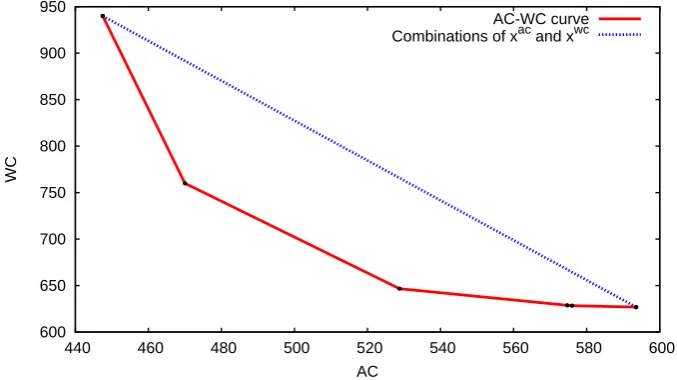
The average case is then given as cˆ= (63.75,44.75,75.50,47.00). An optimal solution to the average case is thereforexac:= (0,10,0,0) with an average case
is not robust, as it only uses a single item. An optimal worst case solution xwc:= (5.50,3.15,1.35,0.00)on the other hand has a worst case perfomance of 626.9 and an average case performance of593.5.
[image:5.595.125.464.295.485.2]A feasible method to generate a solution that yields a compromise between average case and worst case performance is to choose a convex combination of solution xac andxwc. The solutions values of these combinations are shown in
Figure 1.
But by calculating the complete AC–WC curve, also presented in Figure 1, we can make a more detailed analysis of the trade-off between average and worst case performance of these solutions. In particular, we can see that already a small loss in worst case performance may yield a large improvement in average case performance, yielding a valuable alternative to the original robust solution. The decision maker can now evaluate which solution he prefers most.
600 650 700 750 800 850 900 950
440 460 480 500 520 540 560 580 600
WC
AC
AC-WC curve Combinations of xac and xwc
Figure 1: Every convex combination of solution xac and xwc yields a feasible solution the corresponding performances of these combinations are shown as the dotted, blue line. The AC–WC curve is shown as the straight, red line.
3
Computing the AC–WC Curve
In the next section we show how we can overcome this drawback. We explain the theoretical principles that allow us to compute the AC–WC curve without solving problems that have the same structure as problem (W C). Instead, we only need to solve problems that maintain the structure of the original problem (LP), and one additional linear master program with easily solvable structure. This has the practical advantage that specialized algorithms for problems of type (LP) can be reused.
3.1
Dantzig-Wolfe Decomposition in the Objective Space
In [2] it is shown that the set of efficient solutions of the problem
vec−min (cT1x, . . . , cTnx)
s.t. Ax=b
x≥0
contains an optimal solution for (W C). Following a similar idea, we introduce a second multicriteria optimization problem besides problem (BILP). It uses the same constraints as problem (LP) but the objective function is lifted to a vector valued function that represents the performance in every scenario as well as the performance in the average case scenario. So, we get a (n+ 1)−criteria optimization problem (M OLP).
vec−min (cT1x, . . . , cTnx,ˆcTx)
s.t. Ax=b (MOLP)
x≥0
Denote byPM OandPBI the set of all Pareto efficient solutions of problems (M OLP) and (BILP), respectively. Note that a solution of problem (BILP) is a tuple of the form (x, z). Nevertheless we can identify all Pareto efficient solutions of problem (BILP) with thexcomponent, as componentzis uniquely determined byx. We arrive at the following first observation.
Lemma 3.1. PBI⊆ PM O
Proof. Let x be an arbitrary element of PBI. Hence, for all solutions x0 of problem (BILP) with ˆcTx0<ˆcTxit follows that the worst case performance of
x0 is worse than that ofx, i.e. ∃k:cT kx
0 > cT
kx. We assume thatx6∈ PM O. It is trivial thatxis feasible for (M OLP), hence, there must exist a solution
x00 of (M OLP) with cT
ix00 ≤ cTi x for i = 1, . . . , n and ˆcTx00 ≤ ˆcTx where at least one inequality is strict. Summing up over all scenarios we get that ˆ
cTx00 = 1
n Pn
i=1c
T ix00 <
1
n Pn
i=1c
T
i x = ˆcTx. As x00 is feasible for (BILP) it follows from the efficiency property of xthat ∃k:cT
kx00> cTkx, which yields a contradiction.
In the following we use the assumption that the set of feasible solutions
X ={x∈RN |Ax=b, x≥0} is bounded. Therefore, there exists a finite set
X0={x0
1, . . . , x0s}of vertices ofX such thatX =conv{X0}, whereconvdenotes the convex hull of a set of points.
Proof. Letx be an arbitrary element ofPM O. Asx∈ X it follows that∃I ⊆
{1, . . . , s}, λ ∈R|>I|0 : x=P
j∈Iλjx0j and P
j∈Iλj = 1. Assume that∃k∈ I :
x0k∈ P/ M O. From this follows that there must exist another feasible solution ˆxk that dominatesx0k, i.e. cT
ixˆk≤cTix0kfori= 1, . . . , nand ˆcTxˆk ≤cˆTx0k where at least one inequality is strict. Asλk>0 it follows that ˆx=Pj∈I\{k}λjx0j+λkxˆk dominatesx, which is a contradiction. Therefore, the assumption was wrong and it holds that∀i∈I:x0i∈ PM O. Hence, it follows that{x0j |j∈I} ⊆ PM O∩ X0. Therefore,x∈conv{{x0j|j∈I}} ⊆conv{PM O∩ X0}.
We define the set of Pareto efficient vertices of the polytopeX byP0
M O =
PM O∩ X0 and the linear mapC(x) = (cT1x, . . . , c
T nx,ˆc
Tx)T. The next lemma is a direct consequence of Lemma 3.1 and Lemma 3.2.
Lemma 3.3. C(PBI)⊆conv{C(PM O0 )}
Proof. It holds thatC(PBI)⊆C(PM O)⊆C(conv{PM O0 }) =conv{C(PM O0 )}. The first and second step follow from Lemma 3.1 and Lemma 3.2 and the last step uses the linearity of mapC.
Next consider the parametric problem (λ−ACW C) (λ∈[0,1]) that opti-mizes a weighted sum of average and worst case performance.
minλˆcTx+ (1−λ)z
s.t. cTkx≤z k= 1, . . . , n (λ−ACW C)
Ax=b
x≥0
Observation 3.4. TheAC−W C curve can be computed by solving a sequence of (λ−ACW C) problems, whereλ∈[0,1].
To see that Observation 3.4 holds we refer to [14]. The authors of [16] deal with the approximate computation of the Pareto front of bicriteria optimization problems. They define the algorithms SANDWICH and −SANDWICH that can be used to compute the complete Pareto front of a bicriteria problem respec-tively only a set that approximates this Pareto front. As the exact description of SANDWICH and−SANDWICH is beyond the scope of this paper we refer to [16] for more information. The crucial observation for our theoretical result is that the application of these algorithms in our context leads to a sequence of (λ−ACW C) problems.
The main idea is to translate problem (λ−ACW C) into the objective space of problem (BILP). We use variables a and z, where arepresents the average case andzthe worst case performance.
minλa+ (1−λ)z
s.t. yn+1=a (OBJ)
yi≤z i= 1, . . . , n
y∈C(PBI)
We define a new problem (OBJ0) by replacingC(P
conv{C(P0
M O)} due to Lemma 3.3, it is evident that (a∗, z∗, y∗) is feasible for (OBJ0). On the other hand, for every optimal solution (a∗∗, z∗∗, y∗∗) of (OBJ0) it must hold thaty∗∗ ∈C(PBI). Hence, the optimal objective values of (OBJ) and (OBJ0) are equal.
minλa+ (1−λ)z
s.t. yn+1=a (OBJ0)
yi≤z i= 1, . . . , n
y∈conv{C(PM O0 )}
If we know the set C(P0
M O) ={y
1, . . . , yr} completely, we can reformulate the problem in the following way.
minλa+ (1−λ)z
s.t.yˆ= r X
i=1 αiyi
r X
i=1 αi= 1
ˆ
yn+1=a
ˆ
yi≤z i= 1, . . . , n
α≥0
Introducing slack variables and removing the superfluous variable ˆy we get the parameterized master program (λ−M).
minλa+ (1−λ)z
s.t. −1 .. . −1 0 .. . 0 1 . .. 1 y1 1 .. . y1 n . . . yr 1 .. . yr n
0 −1 0 yn1+1 . . . yrn+1
0 0 0 1 . . . 1
z a s1 .. . sn α1 .. . αr = 0 .. . 0 0 1
(z, a, α, s)≥0
Theorem 3.5. TheAC−W Ccurve can be computed by solving linear programs of the form (λ−M)and instances of the original problem(LP).
3.2
Algorithmic Details
In this section we discuss the benefits and the drawbacks of solving (λ−M) using column generation instead of (λ−ACW C) directly as linear programs. The most obvious benefit is the fact that the original problem structure (LP) remains preserved. Hence, the column generation approach is especially useful if there exist specialized algorithms for problem (LP) that allow to solve (LP) faster than it could be solved by linear programming solvers (e.g., one can use the network simplex algorithm to solve uncertain network flow problems). But note that it is necessary to solve several problems of type (LP) to solve a single (λ−M) problem – for every column we generate in the master program, we need to solve one subproblem. To solve (λ−ACW C) directly we have only to solve a single linear program.
The drawback of the column generation approach to generate a possibly large number of columns to solve problem (λ−M) can be compensated by the fact that columns that are generated to solve (λ−M) can be reused in the master program to solve another problem (˜λ−M). This makes the column generation approach valuable for computing the AC–WC curve, as in the SANDWICH algorithm a probably long sequence of these problems (λ−M) needs to be solved for different values ofλ.
In the case where computation time is limited and, therefore, one cannot compute the complete AC–WC curve, another benefit from the column gen-eration approach can be obtained. If the SANDWICH algorithm is stopped prematurely, an incomplete set of Pareto efficient solutions is provided by the algorithm. Using the column generation approach one can still try to gener-ate some additional Pareto efficient solutions by solving the remaining (λ−M) problems heuristically using only the columns that were generated so far. As the restricted programs (λ−M) can be solved effectively even for a large number of columns due to the relatively small number of rows, the heuristic solution of (λ−M) needs little additional computation time.
The performance of the column generation method depends heavily on the number of scenarios. Whereas one additional scenario increases the dimension of the Pareto front of (M OLP) and also the number of rows of (λ−M) by one, the additional scenario can be represented by just one additional inequality in the linear programming formulation of (λ−ACW C). Hence, one can expect the column generation approach to perform relatively well for a small number of scenarios and relatively badly for a large number of scenarios.
4
Experiments
4.1
Setup and Instances
ua is the capacity of flow that can be sent over arc a ∈ A, and bv is the supply/demand of node v ∈V. The goal is to find a flow with minimal costs that fulfills the capacity constraints on all arcs as well as the supply and the demand constraints of every node. This well-known problem can be stated as the following linear program
minX a∈A
caxa
s.t. X
a∈δ+(v)
xa− X
a∈δ−(v)
xa=bv ∀v∈V
0≤xa ≤ua ∀a∈A,
where we denote byδ+(v) (δ−(v)) the set of all arcs leaving (entering) nodev. The instances for the minimum cost flow problems are generated randomly. We consider two types of instances: One with discrete uncertainty, and one with interval-based uncertainty. The instances R with discrete cost scenarios are described by six parametersR-N-p-n-cmax-umax-bmax. The number of nodes is given by N. We create an arc between two arbitrary nodes with probability
p. The number of different scenarios is given byn. The costscj(a) of an arca in scenarioj are generated by the formula
cj(a) = (
Y ·cmax· jn 2
,ifD≤ 1 2 Y ·cmax· n−nj
2
,else ∀a∈A, j= 1, . . . , n,
where Y and D are independent and uniformly distributed in [0,1]. We use this formula to generate a cost structure with varying spreads. The capacityua of an arc a is set to umax for all arcs. The supply/demand bv of a node v is chosen uniformly from the interval [−bmax, bmax], except for the supply/demand
bvN =−
P
v6=vNbvof the last nodevN. Note that the choice ofbvN is necessary
to get a feasible minimum cost flow instance.
The instancesIwith interval uncertainty for the arc costs are also described by six parametersI-N-p-var-cmax-umax-bmax. The parametersN, p, umax, and
bmaxare used in the same way as forRinstances to generate the arcs and their capacities as well as the nodes and their corresponding demands/supplies. The average costs ˆc(a) of an arcaare chosen uniformly at random from the interval [0, cmax]. Next, the worst case cost c(a) of an arc a are chosen uniformly at random from the interval [ˆc(a),ˆc(a)(1 +var)].
All experiments were conducted on an Intel Core i5-3470 processor, running at 3.20 GHz, 8 GB RAM under Windows 7. The linear and quadratic programs (see Section 4.3.2) are solved with CPLEX version 12.6. The minimum cost flow problems are solved with the network simplex algorithm of the LEMON graph library [9] version 1.3.1. Algorithms were implemented with Microsoft Visual C++ 2010 Express.
4.2
Computation of the AC–WC curve
4.2.1 Exact Computation
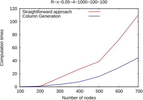
introduced in this paper that is based on column generation. We compare the times needed for both algorithms to compute the complete AC–WC curve.
In the first experiment, we fix the underlying graph of the minimum cost flow problem and vary the number of scenarios. In the second experiment, we fix the number of scenarios and vary the number of nodes in the graph. The values are averaged over 10 runs per instance.
0 2 4 6 8 10 12 14 16
2 3 4 5 6 7
Computation times
Number of scenarios R−300−0.05−x−1000−100−100
Straightforward approach Column Generation
(a) All graphs are of the typeR-300-0.05-x-1000-100-100. Thex-axis shows the different number of scenarios and they-axis the time (in seconds) needed to compute the complete AC–WC curve.
0 20 40 60 80 100 120
100 200 300 400 500 600 700
Computation times
Number of nodes R−x−0.05−4−1000−100−100
Straightforward approach Column Generation
[image:11.595.169.407.422.589.2](b) All graphs are of the typeR-x-0.05-4-1000-100-100. Thex-axis shows the different number of nodes and they-axis the time (in sec-onds) needed to compute the complete AC–WC curve.
Figure 2: Comparison of computation times.
scenarios can lead to a decreasing number of solutions that need to be computed to represent the AC–WC curve.
The second experiment (Figure 2(b)) confirms that the column genera-tion approach outperforms the straightforward approach if the instance size increases, assuming that the number of scenarios is small.
4.2.2 Approximate Computation
As the number of solutions that need to be computed to represent the AC–WC curve is not polynomially bounded in the input size, the exact computation of the AC–WC curve might be an unreasonable approach. This problem can be resolved in practice by computing only a subset of these solutions.
Denote byP the set of all points of the AC–WC curve. We call a setS⊆P
an−AC–WC curve if∀p∈P ∃s∈S:sac≤(1 +)pac andswc≤(1 +)pwc. For any practical application one should be able to choose an appropriate
such that the −AC–WC curve is sufficient in comparison to the AC–WC curve. Note that there exist efficient algorithms to compute the −AC–WC curve. We use the −SANDWICH algorithm [16] that is very similar to the SANDWICH algorithm. The main difference is the choice of the weights used for the weighted sum computations. We used the column generation method to solve the weighted sum problems that have to be solved during the execution of the−SANDWICH algorithm.
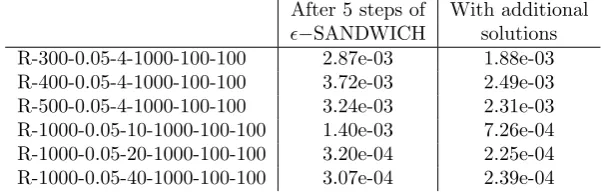
We did three different experiments. In the first experiment we bounded the running time of the−SANDWICH algorithm by a multiple of the time needed to compute the average and worst case solution. In the second experiment we bounded the number of iterations used in the−SANDWICH algorithm. In the last experiment we stopped the generation of new columns after 5 steps of the algorithm (where one step of the−SANDWICH algorithm corresponds to the exact solution of one (λ−ACW C) problem) and solved all remaining weighted sum problems only approximately by solving the restricted master program.
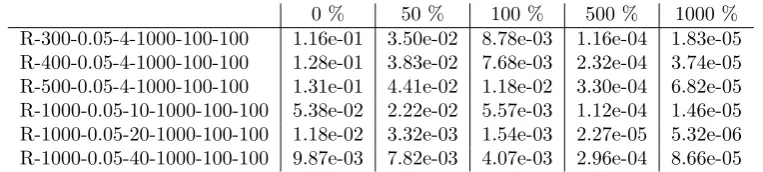
Note that the set consisting only of the average and worst case solution is also an −AC–WC curve for an that is sufficiently large. The values are averaged over 10 runs per instance.
[image:12.595.106.488.528.614.2]0 % 50 % 100 % 500 % 1000 % R-300-0.05-4-1000-100-100 1.16e-01 3.50e-02 8.78e-03 1.16e-04 1.83e-05 R-400-0.05-4-1000-100-100 1.28e-01 3.83e-02 7.68e-03 2.32e-04 3.74e-05 R-500-0.05-4-1000-100-100 1.31e-01 4.41e-02 1.18e-02 3.30e-04 6.82e-05 R-1000-0.05-10-1000-100-100 5.38e-02 2.22e-02 5.57e-03 1.12e-04 1.46e-05 R-1000-0.05-20-1000-100-100 1.18e-02 3.32e-03 1.54e-03 2.27e-05 5.32e-06 R-1000-0.05-40-1000-100-100 9.87e-03 7.82e-03 4.07e-03 2.96e-04 8.66e-05
Table 1: The numbers in the columns 2-6 give the approximation guarantee
0 1 5 10 100 R-300-0.05-4-1000-100-100 1.16e-01 5.12e-02 2.87e-03 8.07e-04 6.16e-06 R-400-0.05-4-1000-100-100 1.28e-01 5.48e-02 3.27e-03 8.50e-04 7.50e-06 R-500-0.05-4-1000-100-100 1.31e-01 4.98e-02 3.24e-03 7.02e-04 8.43e-06 R-1000-0.05-10-1000-100-100 5.38e-02 2.61e-02 1.40e-03 3.93e-04 3.51e-06 R-1000-0.05-20-1000-100-100 1.18e-02 6.47e-03 3.20e-04 8.20e-05 1.02e-07 R-1000-0.05-40-1000-100-100 9.87e-03 4.30e-03 3.07e-04 8.97e-05 7.48e-07
Table 2: The numbers in the columns 2-6 give the approximation guarantee
of the−AC–WC curve that can be obtained depending on the number of steps of the−SANDWICH algorithm.
After 5 steps of With additional
−SANDWICH solutions R-300-0.05-4-1000-100-100 2.87e-03 1.88e-03 R-400-0.05-4-1000-100-100 3.72e-03 2.49e-03 R-500-0.05-4-1000-100-100 3.24e-03 2.31e-03 R-1000-0.05-10-1000-100-100 1.40e-03 7.26e-04 R-1000-0.05-20-1000-100-100 3.20e-04 2.25e-04 R-1000-0.05-40-1000-100-100 3.07e-04 2.39e-04
Table 3: The numbers in the second column give the approximation guar-antee of the −AC–WC curve that can be obtained within 5 steps of the
−SANDWICH algorithm. The third column gives the improved guarantee af-ter additional solutions are computed using the already generated columns of the master programs (λ−M).
Discussion. The second column in Table 1 and Table 2 describes how well the AC–WC curve is approximated by the set that consists only of the average and worst case solution. We observe that an increasing number of scenarios improves the approximation guarantee of the average and worst case solution. We observe in general that already relatively few steps of the − SANDWICH algorithm suffice to get a −AC–WC curve with a good approximation guarantee. Note especially the values for in Table 1. They indicate that the time needed to compute a reasonable good−AC–WC curve is in the same order as the time needed to compute the average and worst case solution. In a practical setting this means that whenever one is able to compute the average and the worst case solution of a problem, one should also be able to compute an −AC–WC curve that provides on the one hand clear insight in the different trade-offs between average and worst case objective and on the other hand a rich set of alternative solutions where the decision maker can choose from.
[image:13.595.145.446.281.377.2]4.3
Properties of the AC–WC curve
In the first part of this section we show how the AC–WC curve can be used to find compromise solutions that are reasonable for the average and the worst case objective. In the second part we compare two common robustness concepts and measure how they perform in comparison with the AC–WC curve.
4.3.1 Gains by using the AC–WC curve
In this section we compare the trade-offs between the average case and the worst case solution. We use the AC–WC curve to answer the questions: Starting from the worst case solution, allowing the worst case value to increase, by how much can we decrease the average case value? And vice versa: Starting from the average case solution, allowing the average case value to increase, by how much decreases the worst case value? The numbers in the tables are averaged over 100 runs per instance.
[image:14.595.148.448.320.464.2]WC value increased by +0.1 % +1.0 % +5.0 % +10 % R-200-0.05-2-1000-100-100 99.80 98.06 91.34 84.94 R-200-0.05-3-1000-100-100 99.88 98.86 95.26 92.48 R-200-0.05-4-1000-100-100 99.90 99.08 96.43 94.42 R-200-0.05-5-1000-100-100 99.92 99.32 97.58 96.34 R-200-0.05-6-1000-100-100 99.92 99.35 97.99 97.17 R-300-0.05-2-1000-100-100 99.77 97.72 89.81 82.37 R-300-0.05-3-1000-100-100 99.83 98.39 93.25 89.24 R-300-0.05-4-1000-100-100 99.88 98.89 95.62 93.21 R-300-0.05-5-1000-100-100 99.90 99.06 96.46 94.46 R-300-0.05-6-1000-100-100 99.92 99.26 97.32 95.87
Table 4: The numbers in columns 2-5 give the average case performance of a solution that has a higher worst case value than the worst case solution. The average case performance of the worst case solution is normalized to 100.
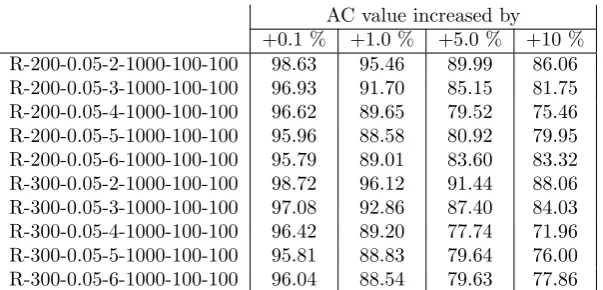
AC value increased by +0.1 % +1.0 % +5.0 % +10 % R-200-0.05-2-1000-100-100 98.63 95.46 89.99 86.06 R-200-0.05-3-1000-100-100 96.93 91.70 85.15 81.75 R-200-0.05-4-1000-100-100 96.62 89.65 79.52 75.46 R-200-0.05-5-1000-100-100 95.96 88.58 80.92 79.95 R-200-0.05-6-1000-100-100 95.79 89.01 83.60 83.32 R-300-0.05-2-1000-100-100 98.72 96.12 91.44 88.06 R-300-0.05-3-1000-100-100 97.08 92.86 87.40 84.03 R-300-0.05-4-1000-100-100 96.42 89.20 77.74 71.96 R-300-0.05-5-1000-100-100 95.81 88.83 79.64 76.00 R-300-0.05-6-1000-100-100 96.04 88.54 79.63 77.86
[image:14.595.148.450.531.676.2]Discussion. The most obvious observation by comparing Tables 4 and 5 is the fact that almost all numbers of Table 4 are bigger than the corresponding numbers of Table 5. This yields to the following statement. Decreasing the worst case value of the average case solution is cheaper than decreasing the average case value of the worst case solution. Small increases of the average case value of the average case solution guarantee in most cases already considerably decreases of the worst case value. But also an increase of the worst case value of the worst case solution of x% can lead to reductions of the average case value that are above x%. Note that an increasing number of scenarios reduces this positive effect.
4.3.2 Comparison with Other Robustness Concepts
In contrast to the other experiments where we assumed to have a discrete un-certainty set, we consider interval unun-certainty in this section. This kind of uncertainty is typical if the data is obtained, e.g., by measurements. Also more general versions of uncertainty sets are studied in the literature, e.g. polyhedral or ellipsoidal uncertainty sets [5]. These uncertainty sets are important if the values of the parameters are correlated and, therefore, a hyperrectangle is not the correct form for the uncertainty set.
The drawback of interval uncertainty or continuous uncertainty sets in gen-eral is that the uncertainty sets can contain very unlikely scenarios and, there-fore, solutions that should perform well for all scenarios in these uncertainty sets are in general over-conservative and perform bad in the average case. Therefore, researchers have tried to find robustness concepts that improve the average case performance of the solution and still give a rather good protection against most realizations of the uncertainty set.
Note that most robustness concepts normally only deal with uncertainty in the constraints and not in the objective function, as it is claimed that the objective function can be represented by a constraint.
The goal of this section is to compare two different robustness approaches that define a parameter that helps the modeler to control the conservatism of the solution with the AC–WC curve. We analyze if the transformation of an uncertain objective to an uncertain constraint has undesired side effects. As benchmark problem we use the minimum cost flow problem on randomly generated graphs.
Γ−Robustness. The concept of Γ−robustness was introduced by Bertsimas and Sim [8]. They motivate their concept by the observation that the situation where all parameters take their worst case value simultaneously should be rather unlikely. Hence, they propose to use a parameter Γ that defines an upper bound for the number of parameters that can deviate from their nominal value.
prob-lem leads to the following linear program.
minX a∈A ˆ
caxa+pa+ Γz (Γ−P)
s.t. X
a∈δ+(v)
xa− X
a∈δ−(v)
xa=b(v) ∀v∈V
(ca−cˆa)xa ≤pa+z ∀a∈A 0≤xa ≤ua ∀a∈A
0≤pa ∀a∈A
0≤z
Controlling parameter Γ allows the modeler to control the conservatism of the solution. If Γ is chosen to be 0, z can be chosen arbitrary large in an optimal solution and, therefore, pa = 0 ∀a ∈ A. In this case the objective function is equal to the average case objective function ˆcTx. If, on the other hand, Γ is chosen to be as large as the number of uncertain parameters, z = 0 in an optimal solution andpa= (ca−ˆca)xa ∀a∈A. Hence, the objective function is equal to the worst case objective functioncTx.
Ω−Robustness. The second concept was proposed by Ben-Tal and Nemirovski [6]. We call it Ω−robustness as the problems are parameterized by Ω. The main idea of the concept is to include chance constraints to deal with possible con-straint violations. There might exist a parameter realization such that a feasible solution of the Ω–robust problem is infeasible for the original problem. How-ever, the probability that such a parameter realization happens should be small under the assumption that the parameters are distributed symmetrically and independently. Additionally, a value κhas to be specified as a bound for the probability of constraint violation. Ben-Tal and Nemirovski showed how the probability constraint can be relaxed by a second order cone constraint. The valueκis then replaced by Ω =p−2ln(κ). The application of the Ω-robustness concept to the minimum cost flow problem leads to the following quadratically constraint program.
minX a∈A
caxa−(ca−cˆa)za+ Ωq (Ω−P)
s.t. X
a∈δ+(v)
xa− X
a∈δ−(v)
xa=b(v) ∀v∈V
X
a∈A
(ca−cˆa)2za2≤q
2
0≤za≤xa ≤ua ∀a∈A 0≤q
Ignoring the relation between Ω and κ one can interpret Ω as a parameter that can be used to control the conservatism of the solution. If Ω is set to 0,
enough values for Ω, za = 0 ∀a∈Ain an optimal solution and, therefore, the objective function is equal to the worst case objective functioncTx.
Hence, we see that the parameter Ω plays a similar role for Ω−robustness as Γ for Γ−robustness.
Experiment description. For every set of parameter values we generate 5 graphs and compute for each the AC–WC curve. We define the Γ\Ω−curves as all points that are obtained by solving (Γ−P)\(Ω−P) if Γ\Ω is integral. To compute the Γ\Ω−curves we set Γ\Ω = 0 and compute the solution of (Γ−P)\(Ω−P). Next, we increase both parameters by 1 and resolve the problem. We repeat this process until an optimal solution of the worst case problem is found. For every solution found so far we compute the average and worst case performance and compare it to the AC–WC curve. As the AC–WC curve is the Pareto front of a minimization problem it is clear that all points of the Γ\Ω−curves must lie on or above the AC–WC curve.
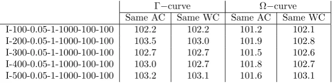
To measure the distance between the AC–WC curve and the Γ\Ω−curves we use two different measures. First we choose the solution of the AC–WC curve that minimizes the sum of average and worst case performance. We call this solution in the following the compromise solution. Next, we select the points from the Γ\Ω−curves that have the same average case performance as the compromise solution and compare the worst case performance of these points with the worst case performance of the compromise solution. We repeat this step and compare the average case performances if we require equal worst case performance. The values obtained by this computation indicate how close the Γ\Ω−curves is to the center of the AC–WC curve.
As second measure we use a more pessimistic measurement to represent the maximum distance between the Γ\Ω−curves and the AC–WC curve. Ev-ery point of the Γ\Ω−curves could become a point of the AC–WC curve if it would be scaled by a factor of 1
(1+) for large enough. For every point of the
Γ\Ω−curves we compute the smallestsuch that the scaled version of the point belongs to the AC–WC curve. To measure the furthest distance between the curves we take the maximum over all such computed’s.
[image:17.595.125.467.536.622.2]Γ−curve Ω−curve Same AC Same WC Same AC Same WC I-100-0.05-1-1000-100-100 102.2 102.2 101.2 102.1 I-200-0.05-1-1000-100-100 103.5 103.0 101.9 102.8 I-300-0.05-1-1000-100-100 102.7 102.7 101.5 102.6 I-400-0.05-1-1000-100-100 103.0 102.7 101.8 102.7 I-500-0.05-1-1000-100-100 103.2 103.1 101.6 103.1
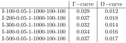
Γ−curve Ω−curve I-100-0.05-1-1000-100-100 0.029 0.012 I-200-0.05-1-1000-100-100 0.037 0.018 I-300-0.05-1-1000-100-100 0.032 0.014 I-400-0.05-1-1000-100-100 0.034 0.016 I-500-0.05-1-1000-100-100 0.037 0.017
Table 7: We scale every point of the Γ\Ω−curves by (1+1). The numbers in columns 2\3 give the smallestsuch that every scaled point of the corresponding Γ\Ω−curves lies below or on the AC–WC curve.
Discussion. Assume that instead of computing the AC–WC curve one would rely on Γ\Ω−robustness. If one is asked to provide a solution that has a certain average case or worst case performance one would provide in most cases a solu-tion that is strictly dominated by a point of the AC–WC curve. The resulting loss is given in Table 6 where theac−wcsolution defines the demanded average or worst case performance. We see that if a fixed worst case value is required both robustness concepts perform almost equally. But if a certain average case value is demanded the Γ−robustness concept provides a solution that is worse in the worst case as the solution provided by the Ω−robustness concept.
The second measure, shown in Table 7, indicates how far the Γ\Ω−curves can deviate from the AC–WC curve. It is obvious that the Ω−curve sticks rather close to the AC–WC curve compared to the Γ−curve.
We conjecture that the relatively bad performance of the Γ−robustness con-cept in this experiment is due to the fact that the underlying minimum cost flow problem tends to generate solutions that are rather dense and the Γ−robustness on the contrary is more effective for problems with sparse solutions.
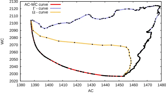
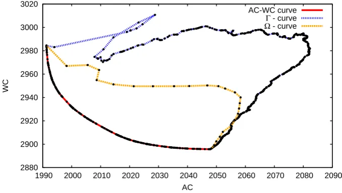
We plot the Γ\Ω−curves and the AC–WC curve for the instancesI-400-0. 05-1.0-1000-100-100 andI-500-0.05-1.0-1000-100-100 in Figures 3 and 4 to visualize the last statements. Note that both robustness concepts generate solutions that are strictly dominated by the worst case solution.
Furthermore, note the different complexities for computing the Ω\Γ\AC– WC curve. A point of the Ω−curve need the solution of a quadratically con-straint program, whereas points of the Γ\AC–WC curve needs the solution of a linear program. Furthermore, the linear program for computing a point of the Γ−curve needsm+ 1 additional variables and 2m+ 1 additional constraints compared with the linear program of the minimum cost flow problem, whereas the linear program for computing a point of the AC–WC curve contains only one additional variable and nadditional constraints. The presented figures are both highly surprising and representative for other instances. They underline the value for the AC–WC perspective in the decision process for a practitioner.
5
Conclusions and Future Research
2020 2030 2040 2050 2060 2070 2080 2090 2100 2110 2120 2130
1380 1390 1400 1410 1420 1430 1440 1450 1460 1470 1480
WC
AC AC-WC curve
[image:19.595.126.465.128.318.2]Γ - curve Ω - curve
Figure 3: The AC–WC curve and the Γ\Ω−curves for an graph of typeI -400-0.05-1.0-1000-100-100. The axis are scaled by 1000.
combined with existing methods from the literature to compute the AC–WC curve efficiently.
Using computational experiments, we found that: Firstly, the newly devel-oped algorithm is effective, especially for a small number of scenarios. Secondly, the time needed to compute a reasonably good approximate version of the AC– WC curve is of the same magnitude as the time needed to compute the average and the worst case solution. Thirdly, the AC–WC curve provides valuable in-formation for a decision maker and allows him to choose the solution that gives the best trade-off between average and worst case performance in his situation. In the last experiment we recall two well-known robustness concepts from literature and use the AC–WC curve to compare them. We observe that the approach suggested by Ben-Tal and Nemirovski is closer to the AC–WC curve than the approach suggested by Bertsimas and Sim. But both approaches reveal a considerable gap to the AC–WC curve.
For future research it will be interesting to compare the described approaches to compute the AC–WC curve with other approaches like the parametric simplex algorithm or the dichotomic method. Furthermore, it is interesting to investi-gate the AC–WC curve of more complex problems that have discrete feasibility sets. Another interesting question is whether the observed gap between common robustness concepts and the AC–WC curve can be re-observed for problems that have a certain objective function but uncertain constraints.
References
[1] R. K. Ahuja, T. L. Magnanti, and J. B. Orlin. Network Flows: Theory, Algorithms, and Applications. Prentice-Hall, Inc., 1993.
2880 2900 2920 2940 2960 2980 3000 3020
1990 2000 2010 2020 2030 2040 2050 2060 2070 2080 2090
WC
AC
[image:20.595.125.465.127.319.2]AC-WC curve Γ - curve Ω - curve
Figure 4: The AC–WC curve and the Γ\Ω−curves for an graph of typeI -500-0.05-1.0-1000-100-100. The axis are scaled by 1000.
gret versions of combinatorial optimization problems: A survey. European Journal of Operational Research, 197(2):427 – 438, 2009.
[3] A. Ben-Tal, L. El Ghaoui, and A. Nemirovski.Robust Optimization. Prince-ton University Press, PrincePrince-ton and Oxford, 2009.
[4] A. Ben-Tal and A. Nemirovski. Robust convex optimization. Mathematics of Operations Research, 23(4):769–805, 1998.
[5] A. Ben-Tal and A. Nemirovski. Robust solutions of uncertain linear pro-grams. Operations Research Letters, 25:1–13, 1999.
[6] A. Ben-Tal and A. Nemirovski. Robust solutions of linear programming problems contaminated with uncertain data. Mathematical Programming, 88:411–424, 2000.
[7] D. Bertsimas, D. Brown, and C. Caramanis. Theory and applications of robust optimization. SIAM Review, 53(3):464–501, 2011.
[8] D. Bertsimas and M. Sim. The price of robustness. Operations research, 52(1):35–53, 2004.
[9] B. Dezs˝o, A. J¨uttner, and P. Kov´acs. LEMON – an open source C++ graph template library. Electronic Notes in Theoretical Computer Science, 264(5):23 – 45, 2011. Proceedings of the Second Workshop on Generative Technologies (WGT) 2010.
[11] M. Fischetti and M. Monaci. Light robustness. In Robust and online large-scale optimization, volume 5868 of Lecture Note on Computer Sci-ence, pages 61–84. Springer, 2009.
[12] M. Goerigk and A. Sch¨obel. Algorithm engineering in robust optimization.
LNCS State-of-the-Art Surveys, 2015. To appear.
[13] J. Ide and E. K¨obis. Concepts of efficiency for uncertain multi-objective optimization problems based on set order relations. Mathematical Methods of Operations Research, 80(1):99–127, 2014.
[14] H. Isermann. Proper efficiency and the linear vector maximum problem.
Operations Research, 22:189–191, 1974.
[15] P. Kouvelis and G. Yu. Robust Discrete Optimization and Its Applications. Kluwer Academic Publishers, 1997.