for Robust Control Design
Atta Oveisi*, Tamara Nestorović*, Allahyar Montazeri**
* Ruhr-Universität Bochum, Mechanics of Adaptive Systems (MAS), Bochum D-44801, Germany ([email protected]).
** Engineering Department, Lancaster University, Lancaster LA1 4YW, UK ([email protected]).
Abstract: Black-box system identification is subjected to the modelling uncertainties that are propagated from the non-parametric model of the system in time/frequency-domain. Unlike classical H1/H2 spectral analysis, in the recent robust Local Polynomial Method (LPM), the modelling variances are separated to noise contribution and nonlinear contribution while suppressing the transient noise. On the other hand, without an appropriate weighting on the objective function in the system identification methods, the acquired model is subjected to bias. Consequently, in this paper the weighted regression problem in subspace frequency-domain system identification is revisited in order to have an unbiased estimate of the frequency response matrix of a flexible manipulator as a multi-input multi-output lightly-damped system. Although the unbiased parametric model representing the best linear approximation (BLA) of the system in this combination is a reliable framework for the control design, it is limited for a specific signal-to-noise (SNR) ratio and standard deviation (STD) of the involved input excitations. As a result, in this paper, an additional step is carried out to investigate the sensitivity of the identified model w.r.t. SNR/STD in order to provide an uncertainty interval for robust control design.
Keywords: System identification, smart structure, confidence interval, vibration control, uncertainty quantification, subspace method, Monte-Carlo simulation.
1. INTRODUCTION
The motivation behind this work is active vibration control of the hydraulically actuated 7 DOF manipulator modelled in (Montazeri & Ekotuyo 2016; Montazeri et al. 2017). Compared to the typical robots driven by the electric motors, hydraulic actuator robots are more flexible due to the higher loop gains, wider bandwidths, and lightly-damped nonlinear dynamics. This flexibility depends on the parameters such as the weight, the dimension, the payload and speed of the manipulator. This results in induced vibrations both during and after the motion of the robot preventing the precise functioning of the robot. This, in turn, degrades the repeatability of the manipulator, particularly in high-speed applications.
It is proven that the vibration of the single or multi-links robots can be suppressed using the active vibration control techniques. Although the mathematical model of the flexible arm can be obtained using finite element methods, a more viable approach to cope with uncertainties and nonlinearities of the system for both identification and control relies on the data-driven models (Ahmadizadeh et al. 2015; Montazeri et al. 2009). Contrary to the classical identification methods, robust identification algorithms use a priori information on the system and its input-output data to produce a nominal model and its associated uncertainty. A comparative study of three primary robust identification approaches, i.e., Stochastic Embedding, Model Error Modelling, and Set Membership, for a lightly-damped system is studied in (Montazeri et al. 2006). The main disadvantage of using the classical spectral analysis in these works for measuring the
frequency response function (FRF) is that the difference between the measurement noise and the system nonlinearity cannot be distinguished. The measurement noise contributes to the variance error of the estimated FRF while the unmodeled dynamics result in the estimation bias. Variance error is uncorrelated with the input signal (in open loop data collection case), but the bias error strongly depends on the nominal model structure and the input signal design. To address this problem, in this paper a multi-sine input signal in the multi-reference orthogonal experiment setting is designed and tested for multivariable identification of the frequency response matrix (FRM) of the system.
To avoid the shortcomings of the classic methods for estimating the FRM, here a more advanced approach based on the so-called local polynomial method (LPM) is investigated (Pintelon, Barbé, et al. 2011). This technique enables estimation of the FRM of the system using periodic excitations. In the LPM framework, the contribution of the noise leakage is approximated by a local least square problem (Pintelon, Vandersteen, et al. 2011). This results in suppression of the noise leakage (transient) errors in the calculation of the sample mean/covariance matrices. The technical details and MATLAB implementation of the robust
and fast versions of the LPM method can be found in (Pintelon et al. 2012).
2. NONPARAMETRIC MODELLING
2.1 System Description
analysis of this work. The plant is an aluminium beam (440×40×3 mm) that is clamped at one end and attached to a vibration exciter (B&K Type 4809) through a rubber-band on the other end as shown in Fig. 1. Four DuraActTM P-876.A15 piezo-patches are optimally collocated on the beam (Nestorović & Trajkov 2013) and more technical details regarding the setup can be found in (Oveisi & Nestorović 2016b). Two measurement channels are realized by a digital laser Doppler vibrometer (LDV) that is collocated with a CCLD accelerometer. In this setting, only three piezo-actuators are used as the control inputs and the shaker is applied to realise the mismatch disturbance input (Oveisi et al. 2017).
Fig. 1. The test rig used for the system.
2.2 Input Excitation Design
The freedomb of input excitation design for MIMO systems is widely investigated in the literature. Schoukens et al., studied the nonparametric model of the system for various input signals in terms of the minimum time per frequency for reaching to a specified signal-to-noise ratio (also known as time factor), the sensitivity of the model w.r.t. noise/nonlinearity, and signal crest factor (CF), i.e., peak-value over the signal root mean square (Schoukens et al. 1988). It is proven that the random-phase (uniformly distributed over [0 2π) range) multi-sine has features such as the periodicity (no leakage), optimizable CF, minimum time factor, user-defined signal spectra, and no spillover effect. This signal can be formally presented in terms of number of samples , sampling frequency , and spectrum amplitude
as / ∑ / / exp 2 /
, where , and . Here, and exp .
represent the unit imaginary number and the exponential function, respectively. Further to the possibility of quantifying nonlinearities, the major advantage of the multi-sine signal is to achieve a good condition number for the power spectrum of the input signal in the MIMO scenarios. In the context of this paper, the operational frequency range of the system is limited to [0 800] Hz while the sampling frequency is selected to be 8192 Hz. Additionally, the number of discrete lines in the band-limited experiments is selected as 65536 in order to have at least nine samples in the 3dB range of each natural frequency. This requirement is
closely related to the degree of freedom associated with the estimated polynomial in robust LPM scheme explained in Section 2.4. A flat spectrum is assigned for the input excitation with the standard deviation of 0.75 in order to prevent actuator saturation.
2.3 Multi-Reference Experiments
The process of estimating the FRM needs generating a set of multi-sine excitation signals. Compared to multiple single-reference excitations, the multi-single-reference orthogonal experiment has times better frequency resolution. This feature comes with the price of distorted data with transient noise for all of the experiments which is alleviated in the robust LPM (Pintelon, Vandersteen, et al. 2011).
The multi-reference signal is generated using the Hadamard multi-sine approach on four input channels while satisfying radix-2 condition (Pintelon et al. 2012). Mathematically, the single-reference multi-sine is multiplied by Hadamard matrix
1/ where ⨂ , and
1,1; 1, 1 in MATLAB matrix notation. The
multi-reference experiments should be repeated times, where each time, a set of inverters are responsible to realize the gain on each input channel, independently. In contrast to multiple single-reference scenario, the Hadamard multi-sine is resilient w.r.t. linear/nonlinear interference hosted by the actuator (Pintelon, Barbé, et al. 2011). This coupling is shown in the results of the next section.
2.4 Robust Local Polynomial Method
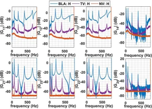
[image:2.595.85.248.229.377.2]As a result of applying the multi-reference periodic signal designed in the previous section, the lightly-damped mechanical structure exhibits both transient and steady state response. Since the transient response is undesirable for FRM identification, it is treated as noise. This is referred to as noise leakage and the robust LPM technique is utilized to suppress its effect in the calculation of the sample mean/covariance matrices. For this purpose, multi-reference modal analyses are performed under full random-phase multi-sine for several realizations. Here, each realization refers to an individual Hadamard multi-sine with several (P) consecutive periods; for which the noise variance is updated by comparing the different periods. The nonlinear variance is also obtained by comparing the response of different realizations (Pintelon, Barbé, et al. 2011). This means that for the test rig shown in Fig. 1, four realizations of the multi-reference Hadamard multi-sine signals are applied (in 16 individual experiments) and ten consecutive periods of the response are recorded. By setting the order of the local polynomial approximation to six and the degree of freedom of the (co-)variance estimates to eight, the robust LPM is used to estimate the FRM and the sample means/covariance matrices of the input/output DFT spectra. The results are summarized in Fig. 2.
BLA of FRM. This indicates that under the ideal laboratory conditions, the variance of FRM is negligible.
Fig. 2. BLA of the FRF using Hadamard multi-sine (H), noise variance (NV), and total variance (TV).
3) The FRFs of the shaker are severely distorted at frequencies higher than 100 Hz. It can be seen that both the noise and nonlinearity levels are high in this case which can be physically justified by the nature of the connection between the shaker and the beam, i.e., rubber band (see Fig. 1). The reason for using a rubber-band instead of direct connection (adhesive wax, screws, etc.) is to match the impedance of the (control) input signals realized by piezo-patches and the (disturbance) signal generated by the electromagnetic shaker (Pintelon et al. 2012).
3. PARAMETRIC STATE SPACE MODELLING
3.1 Black-box subspace system identification
The black-box subspace system identification is based on the estimation of the extended observability matrix from the discrete Fourier transformation (DFT) of the continuous state
space representation , and . If
we measure the FRM of system at 1 discrete normalized frequency
⁄
; 0, … , , then the extended sampled transfer matrix ( ∗ ; 1, … , 1) is used to calculate 2M-point inverse discrete Fourier transformation (IDFT) as in (McKelvey et al. 1996). For user-defined scalars , ∈ that satisfy and , the Hankel matrix is calculated as1 2 ⋯
2 3 ⋯ 1
⋮ ⋮ ⋱ ⋮
1 ⋯ 1
. (1)
where 1 2
∑
2 01 22 , 0, … ,2 1. Hereis the number of highest singular values of Σ that are gathered in Σ such that in the SVD of Σ we have
diag Σ , Σ . Moreover, diag .
denotes the diagonalized vector of entities following the
MATLAB notation. Then, the estimated state matrix
∈
and output matrix∈
arecorrespondingly calculated as 1 † 2 and 3 with . † denoting the Moor-Penrose pseudoinverse and
1
1 1 , 2 1 1 , and
3 1 . The solution for the estimates of the input matrix
∈
and feedthrough matrix∈
is determined by solving the batch least square
problem in , arg min ,
∑ ‖
01
‖
2 where‖
.‖
represents the Frobenius norm (Strang 2016).If the noise model on the measurement output is known ( ), assuming that the elements of are defined (with being the unitary vector in orthonormal space), the DFT of state space equation can be
derived as , and Γ ,
where is the state vector under input and (McKelvey et al. 1996)
1 √
1 2 ⋯
1 2 ⋯
⋮ ⋮ ⋱ ⋮
1 2 ⋯
,
… ,
1 √
⋯ ⋯
⋮ ⋮ ⋱ ⋮
⋯
,
Γ
0 ⋯ 0
⋯ 0
⋮ ⋮ ⋱ ⋮
⋯ ,
diag , , … , ,
(2)
in which and , 1, … , are noise samples on output. Then, for a strongly consistent estimate while →
∞, we define Re Im which satisfies
E Re diag , , … , ∗ in which
has the same form as while replacing with . Assuming that the covariance functions ( ) are known (see previous section), and applying the Cholesky factorization, the matrix ∈ is constructed that satisfies
E for some ∈ (Vakilzadeh et al. 2015). Here E . and Re . represent the expectation operator and real part of a complex-valued matrix, respectively. Then, having , , and in hand, similar to the noise-free output, the system matrices can be estimated using QR factorization of the modified matrix shown in (3)
Re Im
Re Im , (3)
where Im . is the imaginary part of the entity. Then, applying the SVD on 1 22 hands in and system matrices as
, ,
, arg min
, ,
where is calculated by noise variance in the robust LPM of previous section. For implementation of (4), the non-parametric model based on the multi-reference experiments is employed.
3.2 Parametric Model of AVC Benchmark
The singular values in SVD operation is swept between 10 and 22. The process of selecting the correct in (1) is a nontrivial task and despite the rule of thumb ( 5 ), it is recommended to evaluate all candidates in the range of
[image:4.595.304.553.95.224.2]1 10 . The best value of varies for a specific system order . Additionally, the stability of the identified system is investigated in the stability diagram of Fig. 3.
Fig. 3. Stability diagram for black-box subspace system identification: Δ represents stable poles, and x represents unstable poles.
Fig. 3 represents the location and stability of the identified poles for various model order accompanied with two important parameters: a) The best in (1) and (2). b) The associated objective function in (4) for the selected variables and . For each system order , is varied between 1 and 10 and the identification process is repeated. The result of two cases ( 10 and 18) are shown in two subplots in Fig. 3. This illustration is to emphasize the importance of the nontrivial process of selecting . Accordingly, for each system order , the minimum value of the objective function for swept values of is presented in blue font colour and the associated objective values in green font colour. For the cantilever smart beam in Fig. 1, the system order 18 has the minimum value of the objective function with completely stable poles. It should be note that for the results in Fig. 3, no stability constraints are added since no additional information about the structural damping of the system is assumed. On the other hand, if after some structural analysis, the modal damping of the system is calculated, for the price of biased estimation, the constraint identification instead of (4) can be performed in the similar lines as (Miller & de Callafon 2013). The identified model based on the subspace method is compared against the non-parametric FRFs in Fig. 4.
In this figure, a third dotted line is also shown that represents the results of predictive error method (PEM) which is initialized with the identified model from the subspace method (Ljung 1999). In order to shed light on the effect of this model refinement, the pole of the state matrix of the
[image:4.595.42.290.238.378.2]identified models in the discrete domain is presented in Fig. 5.
Fig. 4. Parameterizing the FRFs of the system based on black-box subspace and PE methods.
Both the subspace method, which is a single-step identification approach, and its refinement through PEM, which is based on an iterative optimization technique, have done a great job in fitting the non-parametric frequency-domain data. For output-feedback control design purposes, the rank of controllability and observability matrices are crucial and the identified models have the observability rank of six in both cases and controllability rank of ten and eight for subspace, and PEM, respectively.
Fig. 5. Locations of the poles of the identified models.
4. UNCERTAINTY QUANTIFICATION
[image:4.595.355.501.376.488.2]exhaustive Monte-Carlo simulations are performed in order to approximate these bounds.
A useful method in extracting the confidence intervals of a SISO transfer function model is reported in (Vuerinckx et al. 2001). Two main features of this technique compared to the classical 95 % confidence bound which are also reported in (Pintelon et al. 2007) are 1) the less conservative estimation of the confidence interval for low signal-to-noise ratio (SNR). 2) More accurate bound estimates for high SNR where the uncertainty region associated with each pole/zero of the model may join the uncertainty bounds of others. Developments in the recent years regarding the computational power of the workstations resolves the problem associated with the exhaustive simulations for MIMO systems with large model dimensions.
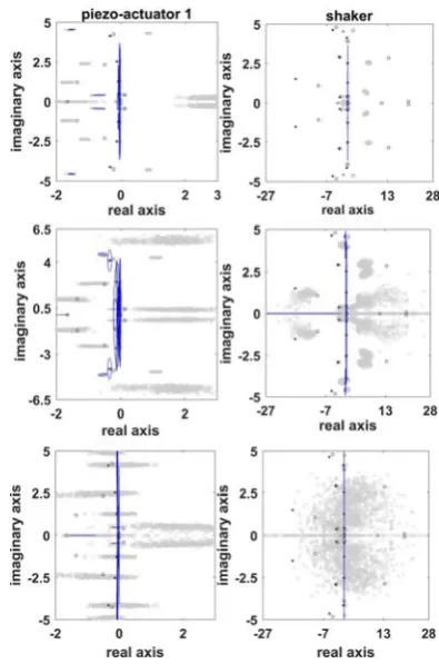
Considering the results for the non-parametric modelling in Fig. 2, where the total variances are 40 dB below the BLAs, and considering the matching quality in Fig. 4, for the application of structural control in Fig. 1, the identified model may be assumed as very accurate. However, in real applications of active vibration control, e.g., robotics in harsh environment (Montazeri et al. 2016), the noise contributions can be significantly higher. Therefore, to investigate the sensitivity of the model, the estimated covariance of the FRM estimates can be used to perturb the non-parametric model with realistic random noise with the normal distribution. For this purpose, three levels of perturbation with the magnitudes of 22 dB (case 1), 18 dB (case 2), and 8 dB (case 3) below the BLA are investigated. Considering the system dimension, 500 Monte Carlo simulation is performed. This requires significantly large system memory and processing power. In each sample, the subspace system identification is carried out on a perturbed BLA with the same 19, 18. In Fig. 6, the variation of the poles and zeros of the system for two inputs (piezo-actuator 1 and shaker) and one measurement output (acceleration) is shown for the sake of conciseness. In this figure, the first, second, and third rows indicate cases 1, 2, and 3, respectively while the nominal values are in black colour and the results from Monte Carlo simulations are shown in gray colour.
Before analyzing the results, it should be pointed out that the poles/zeros with large stability margin are not shown in the range of the real axis (x-axis) since their variation are negligible. From Fig. 6, it can be seen that for high SNR, i.e., case 1, the uncertainties regions on each pole and zero can be distinguished. However, for low SNR (case 3), the regions show interference and an explicit variance estimation of the system poles/zeros are not possible. Unlike the SISO case (not reported here due to the lack of space), the variation of the identified model is not necessarily close to the nominal values (see the uncertainty regions associated with shaker zeros). This issue is closely related to Tustin transformation that is involved in the identification and indicates the sensitivity of the algorithm w.r.t. distortions of poles/zeros close to the imaginary axis in discrete frequency-domain. As reported in (Vuerinckx et al. 2001), the 95 % confidence interval, although may be used as an approximation, represents an inaccurate estimation of the uncertainty bounds. Having the variance of BLA in Fig. 2 in mind, it is naturally
[image:5.595.327.525.97.396.2]observed that the poles and zeros are significantly scattered for the shaker input.
Fig. 6. Variations of poles (*) and zeros (°) of the system and 95 % confidence ellipses for 500 simulations.
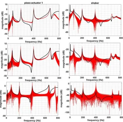
In order to generate a frequency weighting function, for robust control design, which may encompass the modelling uncertainties for various SNR, the parametric FRM is investigated next. The variation of the perturbed model (red lines) are shown around the nominal model (black line) in Fig. 7. The parametrization of the weighting function for , min-max LQG, and -synthesis can be done in a similar lines as (Montazeri et al. 2011; Oveisi & Nestorović 2016a). It is clear from Fig. 7, that due to the introduced perturbations, the identification algorithm is unable to capture the FRM of the system regarding the first natural frequency. This explains the bias of the results in Fig. 6 where some of the poles/zeros are not distributed around the nominal values.
5. CONCLUSIONS
Fig. 7. Variation of FRM for different SNR
ACKNOWLEDGEMENTS
The work is supported by the Engineering and Physical Sciences Research Council (EPSRC), grant number EP/R02572X/1, and National Centre for Nuclear Robotics. The authors are grateful for the support of the National Nuclear Laboratory and the Nuclear Decommissioning Authority (NDA).
REFERENCES
Ahmadizadeh, S., Montazeri, A. & Poshtan, J., 2015. Design of minimax-linear quadratic Gaussian controller using the frequency domain subspace identified model of flexible plate. Journal of Vibration and Control, 21(6), pp.1115–1143.
Ljung, L., 1999. System identification : theory for the user, Prentice Hall.
McKelvey, T., Akcay, H. & Ljung, L., 1996. Subspace-based multivariable system identification from frequency response data. IEEE Transactions on Automatic Control, 41(7), pp.960–979.
Miller, D.N. & de Callafon, R.A., 2013. Subspace
identification with eigenvalue constraints. Automatica, 49(8), pp.2468–2473.
Montazeri, A. et al., 2017. Dynamic modelling and parameter estimation of a hydraulic robot manipulator using a multi-objective genetic algorithm. International Journal of Control, 90(4), pp.661–683.
Montazeri, A. & Ekotuyo, J., 2016. Development of dynamic model of a 7DOF hydraulically actuated tele-operated robot for decommissioning applications. In 2016 American Control Conference (ACC). IEEE, pp. 1209– 1214.
Montazeri, A., Esmaeilsabzali, H. & Poshtan, J., 2006. Comparison of different approaches for robust identification of a lightly damped flexible beam. In
14th European Conference on Signal Processing.
Florence, Italy: IEEE.
Montazeri, A., Poshtan, J. & Choobdar, A., 2009.
Performance and robust stability trade-off in minimax LQG control of vibrations in flexible structures.
Engineering Structures, 31(10), pp.2407–2413. Montazeri, A., Poshtan, J. & Yousefi-Koma, A., 2011.
Design and Analysis of Robust Minimax LQG Controller for an Experimental Beam Considering Spill-Over Effect. IEEE Transactions on Control Systems Technology, 19(5), pp.1251–1259.
Nestorović, T. & Trajkov, M., 2013. Optimal actuator and sensor placement based on balanced reduced models.
Mechanical Systems and Signal Processing, 36(2), pp.271–289.
Oveisi, A., Aldeen, M. & Nestorović, T., 2017. Disturbance Rejection Control Based on State-Reconstruction and Persistence Disturbance Estimation. Journal of the Franklin Institute, 354(18), pp.8015–8037. Oveisi, A. & Nestorović, T., 2016a. Mu-Synthesis based
active robust vibration control of an MRI inlet. FACTA UNIVERSITATIS Series: Mechanical Engineering, 14(1), pp.37–53.
Oveisi, A. & Nestorović, T., 2016b. Robust observer-based adaptive fuzzy sliding mode controller. Mechanical Systems and Signal Processing, 76–77, pp.58–71. Pintelon, R., Barbé, K., et al., 2011. Improved
(non-)parametric identification of dynamic systems excited by periodic signals. Mechanical Systems and Signal Processing, 25(7), pp.2683–2704.
Pintelon, R., Vandersteen, G., et al., 2011. Improved (non-)parametric identification of dynamic systems excited by periodic signals—The multivariate case. Mechanical Systems and Signal Processing, 25(8), pp.2892–2922. Pintelon, R. (Rik), Schoukens, J. (Johan) & Wiley
InterScience (Online service), 2012. System
identification : a frequency domain approach, Wiley. Pintelon, R., Guillaume, P. & Schoukens, J., 2007.
Uncertainty calculation in (operational) modal analysis.
Mechanical Systems and Signal Processing, 21(6), pp.2359–2373.
Schoukens, J. et al., 1988. Survey of Excitation Signals for FFT Based Signal Analyzers. IEEE Transactions on Instrumentation and Measurement, 37(3), pp.342–352. Strang, G., 2016. Introduction to linear algebra Fifth.,
Wellesley-Cambridge Press.
Vakilzadeh, M.K. et al., 2015. Experiment design for improved frequency domain subspace system identification of continuous-time systems. IFAC-PapersOnLine, 48(28), pp.886–891.