warwick.ac.uk/lib-publications
Original citation:
Mourrat, J-C. and Weber, Hendrik. (2017) The dynamic phi^4_3 model comes down from
infinity. Communications in Mathematical Physics, 356 (3). pp. 673-753.
Permanent WRAP URL:
http://wrap.warwick.ac.uk/90705
Copyright and reuse:
The Warwick Research Archive Portal (WRAP) makes this work of researchers of the
University of Warwick available open access under the following conditions.
This article is made available under the Creative Commons Attribution 4.0 International
license (CC BY 4.0) and may be reused according to the conditions of the license. For more
details see: http://creativecommons.org/licenses/by/4.0/
A note on versions:
The version presented in WRAP is the published version, or, version of record, and may be
cited as it appears here.
Mathematical
Physics
The Dynamic
43
Model Comes Down from Infinity
Jean-Christophe Mourrat1, Hendrik Weber2 1 Ecole normale supérieure de Lyon, CNRS, Lyon, France.
E-mail: [email protected]
2 University of Warwick, Coventry, UK.
E-mail: [email protected]
Received: 30 January 2016 / Accepted: 18 July 2017
Published online: 10 October 2017 – © The Author(s) 2017. This article is an open access publication
Abstract: We prove an a priori bound for the dynamic43model on the torus which is independent of the initial condition. In particular, this bound rules out the possibility of finite time blow-up of the solution. It also gives a uniform control over solutions at large times, and thus allows one to construct invariant measures via the Krylov–Bogoliubov method. It thereby provides a new dynamic construction of the Euclidean43field theory on finite volume. Our method is based on the local-in-time solution theory developed recently by Gubinelli, Imkeller, Perkowski and Catellier, Chouk. The argument relies entirely on deterministic PDE arguments (such as embeddings of Besov spaces and interpolation), which are combined to derive energy inequalities.
1. Introduction
The aim of this paper is to prove an a priori bound for the dynamic43model on the torus. This model is formally given by the stochastic partial differential equation
∂tX =X−X3+m X+ξ, onR+× [−1,1]3,
X(0,·)=X0, (1.1)
whereξ denotes a white noise overR× [−1,1]3, andmis a real parameter. Our main result, Theorem1.1below, implies that for every p<∞andε >0 sufficiently small, we have
E ⎡ ⎢ ⎣ sup
0<t1
sup
X0∈B− 1 2−ε
∞ √
tX(t)
B−12−ε
∞ p
⎤ ⎥ ⎦<∞.
global existence of solutions for (1.1), but can also be used to construct invariant measures via the Krylov–Bogoliubov method. This last point is particularly interesting, because equation (1.1) describes the natural reversible dynamics for the43quantum field theory, which is formally given by the expression
μ∝exp
−2
[−1,1]3
1 2|∇X|
2+ 1
4X
4−m
2X
2
x∈[−1,1]3
dX(x). (1.2)
The construction of this measure was a major result in the programme of constructive quantum field theory, accomplished in the late 1960s and 1970s [8–10,13,14]. Our main result yields an alternative construction through the dynamics (1.1).
The construction of the dynamics (1.1) in two and three dimensions was proposed in [34], but in the more difficult three dimensional case very little progress was made before Hairer’s recent breakthrough results onregularity structures; the construction of local-in-time solutions to (1.1) was one of the two principal applications of the theory presented in [23]. Hairer’s work triggered a lot of activity: Catellier and Chouk [5] were able to reproduce a similar local-in-time well-posedness result based on the notion of
paracontrolled distributionsput forward by Gubinelli et al. [18]. Yet another approach to obtain solutions for short times, based on Wilsonianrenormalisation groupanalysis, was given by Kupiainen [30]. The analysis presented in this article is based on the paracontrolled approach of [5,18]. The emphasis is on deriving an a priori estimate that complements the local solution theory and rules out the possibility of finite time blow-up. Our method relies solely on PDE arguments, such as energy inequalities and parabolic regularity theory.
The main difficulty in dealing with (1.1) or (1.2) is the irregularity ofX, which in turn stems from the roughness of the white noise termξ. Realisations of X are distribution valued, so that there is a priori no canonical interpretation of the non-linear termsX3in (1.1) andX4in (1.2). The construction ultimately involves a renormalisation procedure which amounts to subtracting some infinite counter-terms. The first important observa-tion that is used to implement this renormalisaobserva-tion, and which lies at the foundaobserva-tion of all of the local solution theories, is thesubcriticalityof (1.1) in three dimensions. To explain this property, let us momentarily consider this equation overRdfor an arbitrary
d 1. Formally rescaling the equation via ˆ
t =λ2t, xˆ =λx, ξˆ =λd2+2ξ, Xˆ =λ2−2dX, mˆ =λ2m,
yields
∂tˆXˆ =Xˆ −λ4−dXˆ3+mˆXˆ +ξ,ˆ (1.3)
whereξˆis a space-time white noise with the same law asξ. This suggests that ford <4, the influence of the non-linear term should vanish as we consider smaller and smaller scales. This corresponds to the well-known fact that the4dtheory issuperrenormalisable
in dimensiond<4.
Based on this observation, the first step to implement the renormalisation in both the approaches using regularity structures or paracontrolled distributions is the explicit construction of several terms based on the solution of thelinearstochastic heat equation1
(∂t−) =ξ. (1.4)
1 Throughout the article, we adopt Hairer’s convention to denote the terms in the expansion by trees: here
The renormalisation, that is, the subtraction of diverging counter-terms, is implemented at this stage. For example, the simplest stochastic objects constructed from are and , which formally play the role of “2” and “ 3”. These objects are constructed by considering a regularised version δof , e.g. the solution obtained by replacingξby its convolution with a smoothing kernel on scaleδ, and then taking the limits asδtends to zero of
2
δ−Cδ and 3δ−3Cδ δ, (1.5)
for a suitable choice of diverging constantCδ. The proof of convergence of these objects makes strong use of explicit representations of the covariance of and of its Gaussianity. In both theories, the full non-linear system (1.1) is only treated in a second step. This step is completely deterministic, with the random terms constructed in the first step treated as an input. The solution X is sought in a space of distributions whose small-scale behaviour is described in detail by the explicit stochastic objects. In both theories, this is implemented by replacing the scalar field X by a vector-valued function whose components correspond to the different “levels of regularity” ofX. The scalar equation (1.1) then turns into a coupled system of equations. This point is at the heart of both methods. The approaches via regularity structures and via paracontrolled distributions then differ significantly. In the regularity structures approach, a local description of the solutionXin “real space” is given, whereas the paracontrolled approach uses tools from Fourier analysis. However, in both approaches, local-in-time solutions X are found by performing a Picard iteration for the system of equations interpreted in the mild sense. We stress that the renormalisation is completely treated at the level of the construction of the stochastic objects based on (1.4), and that no “infinite constants” appear in the deterministic analysis.
All three approaches mentioned above, i.e., regularity structures [23], paracontrolled distributions [5,18] and renormalisation group [30], focus on the problems arising in the analysis of (1.1) on small scales, and devise a powerful method to deal with the so-called ultra-violet divergences. However, extra ingredients are necessary to obtain information on large scales. This already becomes apparent from the fact that the “good” sign of the term −X3 is not used in the construction of local solutions. In fact, the theories would allow for the construction of local-in-time solutions of (1.1) with the sign of the non-linear term reversed, and solutions of this modified equation are expected to blow up in finite time. Moreover, the scaling analysis above suggests that it is the non-linear term−X3that dominates the dynamics on large scales, so that it can no longer be treated as a perturbation.
In situations where the noise is less irregular, there are well-known tools available to obtain large scale information on non-linear equations such as (1.1). In the deterministic case ξ = 0, the non-linear term is known to have a strong damping effect, and the non-linear equation satisfies better bounds than the linearised version: for solutions of (1.1) withξ =0 (started with anL∞initial datum, say), a simple argument based on the comparison principle and the behaviour of the ODEx˙ = −x3+mximmediately yields X(t)L∞ t−
1
2 + 1, where the implicit constant does not depend on the initial datum.
1.1. Formal derivation of a system of equations. The obvious difficulty in developing a solution theory for (1.1) is the fact that the solution X will be a distribution, and that it is unclear how to interpret the non-linear expression−X3. However, as we have explained in the previous section, on small scales X is expected to “behave like” the Gaussian process ; more precisely, we expect thatX− has better regularity than each of the terms separately. Moreover, the detailed knowledge of the covariance and the Gaussianity of can be used to define the “renormalised” products
( )2 and ( )3 ,
via (1.5). In this section, we present a formal computation in the spirit of [5] to reorganise (1.1) into a system that we are able to solve, assuming that we can define the products of the explicit stochastic terms, even if they are distributions of low regularity. For the moment, we will ignore the “infinite constants” and manipulate the equation formally, adopting the following rules:
• Every term has a regularity exponent associated with it. We will say, for example, that the termsX and have regularity(−12)−, i.e. regularity 12−εforεarbitrarily small. All regularities are derived from the regularity of the white noiseξ, which is
(−5 2)−.
• A function of regularityα1>0 can be multiplied with a distribution of regularity
α2<0 ifα1+α2>0, resulting in a distribution of regularityα2. • Convolution with the heat kernel of∂t−increases the regularity by 2.
• Explicit stochastic objects can always be multiplied, irrespective of their regu-larity. The product of stochastic objects of regularity α1 and α2 has regularity min{α1, α2, α1+α2}.
In Sect.1.2, we will give a precise meaning to these statements and discuss in particular how the last of these rules has to be interpreted. There, we will give a rigorous link between the system we derive formally in this section and the original equation (1.1).
For illustration, we briefly show this calculation in the two-dimensional cased =2, sketching a method introduced by Da Prato and Debussche [7]. In dimension 2, the noiseξhas regularity(−2)−, so bothXand have regularity 0−. According to the rules above, we cannot defineX3directly (the regularity being negative), but we can define the square and the cube of , both of which also have regularity 0−. If we make the ansatz X= +Y, thenY solves
(∂t−)Y = −Y3−3Y2 −3Y − +m( +Y). (1.6)
Convolution with the heat kernel increases regularity by 2, so that we expectY to have regularity 2−, which in turn allows us to define all the products on the right hand side. Hence, we can solve (1.6), at least locally in time. We define the solution we seek, as a replacement for (1.1), to beX := +Y.
We now come back to our original problem, posed in three space dimensions. As stated above, in this caseξhas regularity(−52)−, so thatXand have regularity(−12)−, has regularity(−1)−and has regularity(−32)−. Therefore, the simple procedure leading to (1.6) does not suffice, as it would lead toY being of regularity(12)−, which is not enough to define the products on the right-hand side of (1.6). The most irregular term we encounter in this approach, limiting the regularity ofY to(12)−, is the term , so we use it to define the next-order term in our expansion. We introduce , the solution of
which has regularity(12)−, and postulate an expansion of the form
X = − +u, (1.8)
for some hopefully more regularu. Analogously to the two-dimensional case, we write the formal equation satisfied byu:
(∂t−)u= −(u+ − )3+m(u+ − )−
= −u3−3(u− ) +Q(u),
where we introduced the notation
Q(u)=b0+b1u+b2u2,
with
b0=m( − )+( )3−3 ( )2,
b1=m+ 6 −3( )2,
b2= −3 + 3 .
All of these coefficients have regularity(−12)−. Since the regularity of is(−1)−, the regularity ofuis expected to be 1−, so that the productu is still ill-defined a priori.
In order to solve this problem, we use the notion of paraproducts, following [18]. Roughly speaking, the paraproduct of f andg, which we denote by f < g, carries the
high-frequency modes ofg, modulated by the low-frequency modes of f. The product
f gcan be written
f g= f < g+ f = g+ f >g, (1.9)
where f = g carries the resonant interactions between f andg. The striking property of paraproducts is that, on the one hand, the quantities f < g and f > g are always
well-defined, and only the resonant term f = gcan fail to be defined. But on the other hand, whenever the resonant term is well-defined, its regularity is given by thesumof regularities of f andg (as opposed to the minimum). We refer to the appendix for a more precise discussion, in particular PropositionA.7. We use (1.9) with f =u−
andg= , and decomposeuintov+wsolving
(∂t −)v= −3(v+w− )< , (1.10) (∂t−)w= −(v+w)3−3(v+w− ) +Q(v+w), (1.11)
where we write = > + = for concision. The idea is thatv carries the same local irregularity asu, whilewshould have better regularity, namely(32)−instead of 1−. The paraproduct in the right side of (1.10) contains the high-frequency modes of modulated by the low-frequency modes of(v+w− ). It is always well-defined and has regularity
(−1)−. The paraproduct(v+w− )> is also well-defined and has regularity(−1 2)−.
It remains to consider the resonant term
(v+w− )= ,
that is, regularity(−12)−in our case. Sincewis expected to have regularity(32)−, the termw= can be made sense of classically. In extension of our rules, we postulate that we can define = =:
= as a distribution of regularity(− 1 2)−.
It remains to treat the term v = . The key advantage of the decomposition using paraproducts lies in the following commutator estimates, which allow to rewrite this term using explicit graphical terms of low regularity and more regular objects involving
vandw. As a first step, we denote by the solution of
(∂t−) = ( (t =0)=0), (1.12)
that is,
(t)=
t
0
e(t−s) (s)ds. (1.13)
We also write (1.10) in the mild form
v(t)=etv0−3 t
0
e(t−s)(v+w− )< (s)ds.
The behaviour of the heat kernel suggests that the local irregularity of v is that of −3(v+w− )< . In other words, the difference
com1(v, w)(t):=etv0−3 t
0
e(t−s)(v+w− )< (s)ds
+ 3(v+w− )< (t) (1.14)
has better regularity than v itself. (Justifying this relies on Proposition A.16 and on suitabletimeregularity ofv,wand .) We thus decomposev = into
v = = −3(v+w− )< = +com1(v, w)= .
The second of these terms is defined classically, and it only remains to control the first term. Recall that(v+w− ) < carries the high-frequency modes of ,
mod-ulated by the low-frequency modes of(v+w− ). Hence, it is reasonable to expect
(v+w− )< = to have the same local irregularity as
(v+w− ) = ,
where = is a postulated version of the resonant term
= . To be more precise, the domain of the commutation operator
[<,=] :(f,g,h)→(f <g)= h− f(g =h)
can be extended to cases for which the terms appearing in the definition are not well-defined separately (see PropositionA.9), so that
com2(v+w):= [<,=]−3(v+w− ), , (1.15)
is well-defined. Our renormalisation rule is thus given by
−3(v+w− )< = −3(v+w− )
that is,
v = −3(v+w− )
= +com(v, w),
where
com(v, w):=com1(v, w)= +com2(v+w). (1.16) To sum up, we are interested in solutions of the system
(∂t−)v =F(v+w),
(∂t−)w=G(v, w), (1.17)
where FandGare defined by
F(v+w):= −3(v+w− )< , (1.18)
G(v, w):= −(v+w)3−3com(v, w)
−3w = −3(v+w− )> +P(v+w), (1.19)
with
P(v+w)=a0+a1(v+w)+a2(v+w)2, (1.20)
a0=b0+ 3 = −9 = a1=b1+ 9 = ,
a2=b2
withcomdefined by (1.16), (1.14) and (1.15).
1.2. Renormalised system. We now turn to giving a precise meaning to the discussion of the previous section. From now on, we refer to processes represented by diagrams as “the diagrams”. For such a process, we understand the notion of “being of regularityα” as meaning that it belongs toC([0,∞),B∞α ). This definition would have to be modified forξ and , which only make sense as space-time distributions, but we will not refer to these any longer. We refer the reader to Appendix A for the definition and some properties of the Besov spacesBαp. These spaces are more commonly denoted byBαp,q,
but since we do not make use of fine properties encoded by the second integrability index
q, we will always set it equal to∞and drop it in the notation. For the diagram , some additional information on its time regularity will also be needed.
We now discuss briefly in which way the system (1.17) can be linked to the original equation rigorously, and in particular in which sense the products (and resonant terms) of the diagrams of low regularity should be interpreted. The diagrams entering our equations forvandware
, , , = , = , = , (1.21)
as well as , which is defined as the solution of (1.12), that is, as a function of . These quantities, together with their regularity exponent, are summarized in Table1.
The two remaining ambiguous terms in our formal derivation, namely ( )2and , can be defined classically in terms of the more fundamental object = . For , we can
set
:= = +
Table 1.The list of relevant diagrams, together with their regularity exponent, whereε >0 is arbitrary
τ = = =
ατ −12−ε −1−ε 21−ε −ε −12−ε −ε
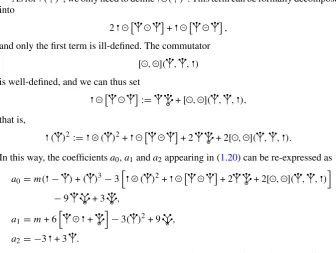
As for ( )2, we only need to define =( )2. This term can be formally decomposed into
2 = < + = = , and only the first term is ill-defined. The commutator
[<,=]( , , ) is well-defined, and we can thus set
= < :=
= +[<,
=]( , , ),
that is,
( )2:= = ( )2+ = = + 2
= + 2[
<,=]( , , ).
In this way, the coefficientsa0,a1anda2appearing in (1.20) can be re-expressed as
a0=m( − )+( )3−3
=( )2+ = = + 2
= + 2[
<,=]( , , )
−9 = + 3 = ,
a1=m+ 6
= +
=
−3( )2+ 9 = ,
a2= −3 + 3 .
Throughout the article, we will never make use of the explicit form of these coefficients, but only that they are of regularity(−12)−.
A natural approach to construct the diagrams in (1.21) is via regularisation: ifξ is replaced by a smooth approximationξδ, then these terms have a canonical interpretation: One can defineδas the solution to (1.4) withξreplaced byξδ,δ:=2δ, δ:=3δ, and δandδas solutions of (1.12) and (1.7) with right hand sidesδandδ. Furthermore, one can then define=
δ =δ=δ,=
δ:=δ=δand=
δ:=δ=δ. Finally, if(vδ,wδ)
solves (1.17), with diagrams interpreted in this way, then indeed,Xδ=δ−δ+vδ+wδ solves (1.1) (withξ replaced byξδ).
However, these “canonical” diagrams fail to converge as the regularisation parame-terδis sent to zero. Given their low regularity, this is not surprising. Yet, the first striking fact about renormalisation is that these termsdoconverge in the relevant spaces if they are modified in a rather mild way. Indeed, if we set
δ =δ, δ=δ−Cδ(1), δ=δ−3Cδ(1)δ,
for a suitable choice of diverging constantCδ(1), then define δand δ as solutions of (1.12) and (1.7) with right hand sides δand δ, and finally
=
δ = δ = δ, =
δ:= δ = δ−3C (2)
δ δ, =
for another choice of diverging constantCδ(2), then these terms converge to non-trivial limiting objects. This is shown in [5], and a very similar result is already contained in [23, Sec. 10] (see also [33] for a pedagogical presentation of these calculations). We stress once more that these results rely heavily on explicit calculations involving variances of the terms involved, which allow to capture stochastic cancellations.
The second striking fact is that the “renormalisation” of these diagrams translates into a simple transformation of the original equation. Indeed, if(vδ, wδ)solves (1.17), with diagrams interpreted in the renormalised way, thenXδ= δ− δ+vδ+wδsolves the identical equation (1.1), withξ replaced byξδbut withrenormalised massive term mδ:=m+3Cδ(1)−9Cδ(2). Since the solution theory for (1.17) is stable under convergence of the diagrams, we can conclude that the solutionXδto this renormalised equation does converge to a non-trivial limit, denoted by X, asδtends to 0.
The fact that we have modified the equation we intended to solve may be discom-forting at first. That this modification is the “correct” one is ultimately justified by the fact that the solutions thus defined are indeed the physically relevant ones. In particular, these solutions arise as scaling limits of models of statistical mechanics near criticality. The connexion between renormalised fields and statistical mechanics has been studied at least since the 1960s (see e.g. [15,16,21] and the references therein). We showed in [31] that the42model can be obtained as the scaling limit of Ising–Kac models near criticality, as anticipated in [12]. Related results were obtained for the KPZ equation, first in [2] via a Cole–Hopf transformation, and then, following [22], in a series of works including [11,17,19,20,27,29]. See also the survey articles [6,24] for a summary of the work on the4model with regularity structures.
1.3. Main result. Our aim is to derive an a priori bound on solutions of (1.1). We will only be concerned with the analysis of the deterministic system. Before we do so, we make a modification to the system (1.17). We give ourselves a (large) constantc0, and consider instead the system
(∂t−)v = F(v+w)−cv,
(∂t−)w=G(v, w)+cv, (1.22)
withFandGas in (1.18) and (1.19) respectively, and with initial condition
v(0)=v0, w(0)=w0. (1.23)
Naturally, this modification changes the definitions ofvandw, but we stress that it does
not change the sumv+w, and therefore the final solutionX. This can easily be seen on the level of the regularised solution(vδ, wδ)discussed in the previous section. Since
(v, w)is the limit of the(vδ, wδ), it follows thatv+witself does not depend on the choice ofc. Therefore, it is ultimately enough to show the existence of a constantcfor which the a priori bound holds. For the same reason, the solutionXdepends onv0and
w0only through the sumv0+w0.
We seek solutions to (1.22) in the spaceXdefined as the set of pairs(v, w)in
C
[0,1],B−
3 5
∞
∩C
(0,1],B
1 2+2ε
∞
∩C18(0,1],L∞
×
C
[0,1],B−
3 5
∞
∩C
(0,1],B∞1+2ε
for which the norm (v, w)X
:=max
sup
0t1
v(t)
B−35
∞
, sup
0<t1
t35v(t)
B12+2ε
∞
, sup
0<s<t1
s12v(t)−v(s)L∞
|t−s|18
,
sup
0t1
w(t)
B−35
∞
, sup
0<t1
t1720w(t)
B1+2ε
∞ ,0<sups<t1s
1
2w(t)−w(s)L∞
|t−s|18
is finite. Here is our main result.
Theorem 1.1(Global existence and a priori bound). For each p ∈ [24,∞)andε >0
sufficiently small, there exist constants c0<∞(depending only on p), C <∞and an
exponentκ <∞such that the following holds. Let K ∈ [1,∞)and let , , , = , = ,
= be distributions such that for every pair(τ, ατ)as in Table1, we have τ ∈C([0,1],B∞ατ), sup
0t1
τ(t)Bατ
∞ K,
as well as
sup
0s<t1
(t)− (s)
B14−ε
∞ |t−s|18
K.
Assume furthermore that the constant c in(1.22)is chosen according to
c=c0K30p. (1.24)
We setv0:=0. For everyw0∈B−
3 5
∞ , there exists a unique pair(v, w)∈Xsolution to
(1.22)–(1.23). Moreover, for every t∈(0,1], we have
w(t)L3p−2
C Kκ
√
t and v(t)B2−p3ε C K
κ.
We now explain how to apply this result to the renormalized solution of (1.1). Note first that the diagrams based on the solution to (1.4) unfortunately do not satisfy uniform bounds such as, for everyp <∞,
sup
s0
E
sup
sts+1
τ(t)Bpατ
∞
<∞, (1.25)
or
sup
r0
E ⎡ ⎢ ⎣ sup
rs,tr+1
(t)− (s)p
B14−ε
∞ |t−s|8p
⎤ ⎥
⎦<∞. (1.26)
However, this problem is very simple to solve: it suffices to add a massive term to the linear equation (1.4), that is, to redefine as the solution to
(∂t −+ 1) =ξ.
applies to this modified system. Moreover, the diagrams defined with a massive term do satisfy (1.25)–(1.26) for every p < ∞. Indeed, this is an elementary extension of the results of Catellier and Chouk [5]; see also [23, Sec. 10] and [33]. We can then apply Theorem1.1iteratively to construct a solution to (1.1) over[0,∞)as follows. We first apply Theorem1.1to define X = − +v+w, where(v, w)solves (1.22) withc
sufficiently large andv0 = 0, w0 = X0 ∈ B−
1 2−ε
∞ . This defines X up to time 1, and
ensures that for every p<∞,
E ⎡ ⎢ ⎣ sup
0<t1
sup
X0∈B− 1 2−ε
∞ √
tX(t)
B−12−ε
∞ p
⎤ ⎥ ⎦<∞,
since for p 24, the spacesL3p−2andB−2p3ε are continuously embedded inB−
1 2−ε
∞ ,
see PropositionA.2and RemarkA.3. We then apply Theorem1.1iteratively at times
t1= 12,t2=1, etc, each time with the new initial conditionv(tk)=0 andw(tk)given
by the sum of thevandwat timetk obtained from the previous iteration. Recall that
this reallocation of the initial condition does not change the sum v +w; nor does a modification of the value of the constantcchange this sum. We thus obtain a solution
Xover[0,∞)which satisfies, for every p<∞,
sup
s0
E ⎡ ⎢ ⎣ sup
s<ts+1
sup
X0∈B
−1 2−ε
∞
(√t∧1)X(t)
B−12−ε
∞ p
⎤ ⎥
⎦<∞. (1.27)
This bound can then be used as the basis for a Krylov–Bogoliubov procedure for the construction of an invariant measure, see [36, Section 4] for the implementation of this argument in the case of the two-dimensional torus.
The two-dimensional analysis in [36] actually yields a stronger statement, namely the exponential convergence to equilibrium with respect to the total variation norm, uniformly over all initial data. The key ingredients are a non-linear dissipative bound akin to (1.27), complemented by the strong Feller property as well as a support theorem. The strong Feller property for (1.1) has in the meantime been established in [26] in the framework of regularity structures, and a support theorem is part of the forthcoming work [28]. We expect that the combination of our main result with these two additional ingredients will indeed imply exponential convergence to equilibrium also in the three-dimensional case.
Remark 1.2.In the simpler two-dimensional case, a comparable analysis was performed in [32]. There, we were able to push the analysis further and show global existence of solutions if the equation is posed on the full spaceR2. The full-space setting is physically more relevant, but also more difficult to analyse, because the stochastic terms lack any decay at infinity, which mandates an analysis in weighted distribution spaces. It would be interesting to investigate whether the methods of [32] can be combined with those of the present article to yield a solution theory for the dynamical4equation in the full spaceR3.
Remark 1.3.At first glance, the choice of initial datum(v0, w0)=(0,X0)may seem surprising. However, we cannot expect to obtain a strong non-linear dissipative bound for the system (1.22) uniformly over all initial data in, sayB−
1 2−ε
∞ ×B−
1 2−ε
ultimately only interested in the sum X = − +v+w, this does not impose any restrictions on the level of the processX.
Remark 1.4.Convergence of lattice approximations to (1.1) was shown in [25] and [37]. This was used in [25] to implement an argument in the spirit of Bourgain’s work on non-linear Schrödinger equations (see e.g. [3]) to show that for almost every initial datum with respect to the measure (1.2), solutions to (1.1) do not explode. This result relies on the analysis of the measure (1.2) performed in [4]. It can then be upgraded using the strong Feller property shown in [26] to obtain the global well-posedness for any initial datum of suitable regularity. We stress however that the spirit of this method is completely different from the method presented here. There, a priori information on the invariant measures is used to rule out finite time blow-up of solutions. Our argument on the other hand relies only on the dynamics, and yields information on the invariant measure as a result.
Remark 1.5.The notion of solution derived in [5] is closely related to (1.17), but slightly different: there, our ansatz
X = − +v+w
is replaced by
X = − + < +,
and a system of equations forand the remainderis solved. The term< in this
decomposition corresponds tovup to a commutator term. Although these approaches are very similar, ours makes the equations solved byvandwmore explicit.
1.4. Sketch of proof and organisation of the paper. We present a local existence and uniqueness result based on a Picard iteration in Sect.2. This result is essentially contained in [5], although we use slightly different norms (see also Remark1.5). The bulk of our argument is contained in Sects.3–7, and we now proceed to explain the strategy. We start by recalling the deterministic argument we aim to mimic. IfX solves the deterministic PDE
∂tX−X = −X3+· · · ,
X(0,·) =X0,
where· · · denotes a collection of lower order terms which is bounded, say in L∞, by
K 1, one can simply test the equation against X3p−3for an even integerpto get the differential inequality
∂tX(t)3Lp3−p−22+X(t)
3p
L3p . . . ,X
3p−3KX(t)3p−3
L3p−3. (1.28)
In fact, an additional “good term”X3p−3|∇X|2(t)L1which comes from the Laplacian
−X on the left-hand side also appears, but we can choose to ignore it. By Young’s and Jensen’s inequalities, the termX(t)3Lp3−p−33 on the right-hand side of the inequality
above can be absorbed into the termX(t)3Lp3p, and then a simple comparison argument for ODEs yields that for everyt>0,
X(t)L3p−2 t− 1 2 +K
This bound is uniform over all initial data X0. A yet simpler manifestation of this
phenomenon is the well-known fact that solutions of the ODEx˙ = −x3satisfyx(t)
(2t)−12 uniformly over all initial data.
We aim to implement a similar testing argument for the system (1.22), which we restate here in the form
(∂t−+c)v= −3(v+w− )< , (1.29) (∂t −)w= −(v+w)3−3com1(v, w)= −3w =
+a2(v+w)2+· · · , (1.30)
where we use the suggestive convention to write
· · · = −3com2(v+w)−3(v+w− )> +a
0+a1(v+w)+cv
for a collection of lower order terms that do not cause any particular difficulty in the analysis. One quickly realises that the testing must be performed on the level of the equation for w. First of all, it is where the “good” cubic term, which is the crucial ingredient for the testing, appears. Second, testing the equation (1.29) againstvwould produce a “good” term proportional to∇v(t)2L2 on the left hand side, but this term is
infinite, since the best regularity exponent we can expect forvis below 1. Moreover, as already hinted at in Remark1.3, since the damping terms(−+c)vin (1.29) are linear, we cannot expectvto relax to equilibrium faster than exponentially. This motivates our choice of initial conditionv0=0 (although in several steps of the argument, it will be useful to estimate the behaviour ofvfor arbitrary initial datumv0).
We proceed to test the equation forwagainstw3p−3for some large even integerp. Ideally, we would like to get a closed expression that permits to invoke an ODE com-parison argument, similar to the one sketched below (1.28). However, several problems present themselves. First, the equations forvandware coupled, so we need to estimate the influence ofvonwand vice versa. Second, even if we controlled all terms involving
v on the right-hand side of (1.30), the testing would not lead to a closed expression: several terms involve higher order regularity information onw, which is not controlled by the “good” termw3p−2|∇w|2L1 appearing when testing the equation. These are
the terms left explicit on the right-hand side of (1.30), namely the termscom1(v, w)= andw = . Indeed, the estimation ofcom1(v, w)= requires information on the time regularity ofw, while the termw= requires one to control at least 1 + 2εderivatives of
w. The quadratic terma2(v+w)2also requires some care because it calls for a control of 12+ 2εderivatives ofvandw, and it is quadratic rather than linear.
A bound onvis presented in Sect.3. The key observation is that although the terms on the right-hand side of (1.29) contain paraproducts with , solutions are relatively easy to control, because bothvandwonly appear linearly. We thus use a Gronwall-type lemma to obtain several estimates onv in terms of the initial datumv0andw. These estimates are used in the following sections to replace all expressions involvingvwhen manipulating the equation forw. The extra massive term−cvappearing on the left-hand side of (1.29) permits to get small constants in this argument. This feature is crucially useful in the testing argument to show that when testing(v+w)3 againstw3p−3, the terms involvingvare dominated by the “good term”w3Lp3p; see Lemma6.3.
sections aim to control the “small-scale behaviour” of solutions, and thus it is natural that the “good sign” of the cubic non-linearity is not used in these sections. The bounds on
vderived in Sect.3are used in these two sections to replace terms involvingvby terms involvingw. In the end, both sups=t|t−s|−
1
8δstwandw(t)
Bγp can be bounded in terms of
t
0 w(
s)3Lp3pds 1
p
, t
0 w(
s)Bp1+4ε
p ds 1
p
, v03
B−3ε
2p ,
as well as a suitable norm forw0. In Sect.6, the equation forwis tested againstw3p−3. We use the bounds onvandδstwfrom Sects.3and4systematically to obtain a bound
onstw(r)3Lp3pdr.
In the concluding Sect.7, this bound is combined with the higher regularity bound on w(t)Bγ
pfrom Sect.5to finish the proof of our main result, Theorem1.1. We first derive a self-contained bound on quantities involvingw, see Lemma7.2. In this estimate, some norm ofvappears on the right-hand side. In order to conclude by mimicking the ODE argument explained below (1.28), we rely on the assumption thatv0 = 0. This is the only place where this assumption is used. We apply the estimate from Lemma7.2up to the first timeτ such thatv(τ)B−3ε
2p exceeds a suitable norm ofw. This argument then yields the desired estimate onw(t)for allt τ. In order to remove the restriction on times to be less thanτ, we use thatt−12 is integrable and Theorem3.1to get a bound on
v(τ)B−3ε
2p , and thus deduce that suitable norms ofw(τ)must be small (irrespectively of the possible smallness ofτ). This final part of the argument only works ifvis measured in a low regularity norm (we work with · B−3ε
2p ; see (7.19)) and this is the reason why throughout the paper we measure the initial datum of the equation forvin this norm.
2. Local Existence and Uniqueness
The aim of this section is to provide a local existence and uniqueness result for the system (1.22). A similar local theory was already presented in [5] in a slightly different formulation (see Remark1.5). The value of the constantcplays no role for the results presented in this section.
We interpret the system (1.22) in the mild sense:
v(t)=et(−c)v0+ t
0
e(t−s)(−c)F(v(s)+w(s))ds, (2.1)
w(t)=etw0+ t
0
e(t−s)[G(v(s), w(s))+cv(s)]ds, (2.2)
and assume our initial condition (v0, w0) ∈ B−
3 5
∞ ×B−
3 5
∞ . (This choice is somewhat arbitrary. Any initial condition of regularity strictly better than−23 would work.) For
T ∈(0,1], we defineXT as the space of pairs(v, w)in
C([0,T],B−
3 5
∞ )∩C((0,T],B
1 2+2ε
∞ )∩C
1
8((0,T],L∞)
×C([0,T],B−
3 5
for which the norm (v, w)XT
:=max
sup
0tT
v(t)
B−35
∞
, sup
0<tT
t35v(t)
B12+2ε
∞
, sup
0<s<tT
s12v(t)−v(s)L∞
|t−s|18
,
sup
0tT
w(t)
B−35
∞
, sup
0<tT
t1720w(t)
B1+2∞ε, sup
0<s<tT
s12w(t)−w(s)L∞
|t−s|18
(2.3)
is finite. The main result of this section is the following.
Theorem 2.1.Letε >0be sufficiently small, let K ∈ [1,∞), and let , , , = , = ,
= be distributions such that for every pair(τ, ατ)as in Table1, we have τ ∈C([0,1],Bα∞τ), sup
0t1
τ(t)Bατ
∞ K (2.4)
as well as
sup
0s,t1
(t)− (s)
B14−ε
∞ |t−s|18
K. (2.5)
(1)For every pair of initial conditions(v0, w0)∈ B−
3 5
∞ ×B−
3 5
∞ , there exists T ∈(0,1]
such that the system(2.1)–(2.2)has a solution(v, w)defined on[0,T). This time T can be chosen maximal, in the sense that either the solution is global, i.e. T=1and the solution can be extend to time t=1and takes values inX1, orlimt↑Tv(t)
B−35
∞ ∨ w(t)
B−35
∞
= ∞, in which case the restriction of(v, w) to any compact interval
[0,T] ⊆ [0,T)takes values inXT. The choice of maximal existence time T and
solution(v, w)with these properties is unique.
(2)If (v0, w0) ∈ B
1 2+2ε
∞ ×B1+2∞ ε, then the solution pair (v, w) constructed in (1) is
continuous at the initial time, in the sense thatXT in the above statement can be
replaced by
XT =
C([0,T],B
1 2+2ε
∞ )∩C18([0,T],L∞)
×C([0,T],B∞1+2ε)∩C18([0,T],L∞).
We start by isolating a bound on the commutatorcom1defined in (1.14), which we
will use again in subsequent sections. We introduce the difference operator
δstf := f(t)− f(s). (2.6) Proposition 2.2(First commutator estimate). Letε >0,β ∈(4ε,1 + 2ε], p ∈ [1,∞]
and T > 0. Under the assumption(2.4)–(2.5), we have for every (v, w) ∈ XT and
t ∈ [0,T),
com1(v, w)(t)−etv0B1+2ε
p K
2
+ t
0
K
(t−s)1+2ε−β2
v(s)Bβ
p+w(s)Bβp
ds
+ t
0
K
(t−s)1+2εδst(v+w)Lpds,
Proof. Recall the definition ofcom1in (1.14). We introduce the commutation operator
[et,<] :(f,g)→et(f < g)− f <(etg), (2.7)
so that
e(t−s)[(v+w− )< ](s)
=(v+w− )(s)<
e(t−s) (s)
+[e(t−s),<](v+w− )(s), (s). (2.8)
We start by estimating the last term in the sum above. The contribution of can be estimated using PropositionA.16:
t
0
[e(t−s),<] (s), (s)ds
B1+2ε
p
t
0
[e(t−s),<] (s), (s)
B1+2p ε ds
t
0
K2
(t−s)34+2ε
dsK2.
By the same reasoning, we have
0t[e(t−s),<]((v+w)(s), (s))ds
B1+2p ε
t
0
K
(t−s)2+32ε−β
(v+w)(s)Bβ
pds.
We now turn to the first term in the right-hand side of (2.8), which we will combine with the last term in (1.14). Recalling (1.13), we observe that
[(v+w− )< ](t)−
t
0 (v
+w− )(s)<
e(t−s) (s)
ds
= t
0
δst(v+w− )
<
e(t−s) (s)
ds.
By PropositionA.7, the · B1+2p ε norm of the integral above is bounded by a constant
times
t
0 δ
st(v+w− )Lpe(t−s) (s)B1+2∞εds
t
0
K
(t−s)1+32ε
δst(v+w− )Lpds,
where we used PropositionA.13and the fact that (s)B−1−ε
∞ 1 in the last step. By the assumption of Hölder regularity in time on (with exponent 18), this last integral is bounded by a constant times
K2+ t
0
K
(t−s)1+32ε
δst(v+w)Lpds,
Proof of Theorem2.1. We follow the usual strategy to first solve the system for some small but strictly positiveT ∈(0,1]using a Picard iteration. In a second step, solutions are restarted iteratively to obtain maximal solutions.
For everyT >0 andM>0, we define the ball
XT,M := {(v, w)∈XT: (v, w)XT M}. For dealing with the case of regular initial data we also introduce the ball
XT,M := {(v, w)∈XT: (v, w)XT M},
where(v, w)X
T is defined in an analogous way to(v, w)XTwithout allowing for blow-up near time 0, i.e.
(v, w)XT
:=max
sup
0tT
v(t)
B21+2ε
∞
, sup
0s<tT
v(t)−v(s)L∞
|t−s|18
,
sup
0tT
w(t)B1+2∞ε sup
0s<tT
w(t)−w(s)L∞
|t−s|18
.
Furthermore, we denote by the fixed point map, i.e. the mapping which associates to
(v, w)∈XT the functiont →(V[v, w], W[v, w])(t), where
V[v, w](
t)=et(−c)v0+ t
0
e(t−s)(−c)F(v(s)+w(s))ds,
W[v, w](
t)=etw0+ t
0
e(t−s)G(v(s), w(s))+cv(s)ds.
We now show that for a suitableMand forT small enough,maps the ballXT,M into
itself and XT,M into itself. The core ingredients are the following bounds, which we
formulate as a lemma.
Lemma 2.3.There exists a constant C depending only on c and K (defined in the assumption of Theorem2.1) such that the following holds. For every
Mmax{1,v0 B−35
∞
,w0 B−35
∞
}, (2.9)
T ∈(0,1],(v, w)∈XM,T and s∈ [0,T], we have
F(v(s)+w(s))B−1−ε
∞ C Ms
−33
100, (2.10)
G(v(s), w(s))+cv(s)
B−12−2ε
∞
C M3s−10099. (2.11)
If
M max{1,v0 B12+2ε
∞
,w0B1+2∞ε}
and(v, w)∈XM,T, then the same bound holds without blow-up near zero, i.e.
F(v(s)+w(s))B−1−ε
∞ C M (2.12) G(v(s), w(s))+cv(s)
B−21−2ε
∞
We momentarily admit this lemma, and first use it to establish thatis a contraction fromXT,M into itself, and also fromXT,M into itself. We focus on the statement
con-cerningXT,M, the proof forXT,M using (2.12)–(2.13) instead of (2.10)–(2.11) being
similar, only simpler.
We start by deriving bounds on V. For every M satisfying (2.9), using Proposi-tionA.13and (2.10), we get that for everyt T andβ∈ {−35,12+ 2ε},
V[v, w](t)
B∞β e
t(−c)v0
Bβ∞+ t
0
1
(t−s)β+1+2 ε
F(v(s)+w(s))B−1−ε
∞ ds
t−12(β+35)v0
B−35
∞
+t10017−β2−ε2M.
Note that the exponents appearing in these bounds are compatible with the exponents appearing in the definition (2.3) ofXT,M. Indeed, forβ = −35 there is no power oft
appearing in front ofv0 B−35
∞
, and the secondt exponent evaluates to 10047 − ε2 > 0.
Forβ = 12+ 2ε, thet exponent beforev0 B−35
∞
evaluates to−1120 −ε > −35 and the
exponent appearing in the second term is−252 −32ε >−35. To bound time differences, we make use of the identity
V[v, w](
t)−V[v, w](s) =(e(t−s)(−c)−Id)es(−c)v0
+(e(t−s)(−c)−Id) s
0
e(s−r)(−c)F(v(r)+w(r))dr
+ t
s
e(t−r)(−c)F(v(r)+w(r))dr,
which holds for any 0 s t. This allows us to write, using PropositionA.13and (2.10) again,
V[v, w](t)−V[v, w](s) L∞
(t−s)18s− 17 40−εv0
B−35
∞
+(t−s)18
t
0
1
(s−r)12( 1 4+1+2ε)
F(v(r)+w(r))B−1−ε
∞ dr
+ t
s
1
(t−r)12(1+2ε)
F(v(r)+w(r))B−1−ε
∞ dr
(t−s)18s−1740−εv0
B−35
∞
+t2009 −εM.
Note that thes-exponent−1740−εappearing in front ofv0 B−35
∞
is strictly larger than
The argument forW is similar: we get W[v, w](
t)B1+2ε
∞
etw0B∞1+2ε+
t
0
1
(t−s)1+22ε+ 1 4+ε
G(v(s), w(s))+cv(s)
B−12−2ε
∞ ds
t−45−εw0
B−35
∞
+t1001 −34−2εM3, (2.14)
as well as
W[v, w](t)
B35
∞
w0 B−35
∞
+t1001 M3,
and
W[v, w](
t)−W[v, w](s)L∞
(t−s)18s− 17 40−εw0
B−35
∞
+(t−s)18M3s 1 100−
3 8−2ε
+ t
s
1
(t−r)14+2ε
M3r−10099dr
(t−s)18s−1740−εw0
B−35
∞
+M3s1001 −38−2ε, (2.15)
where to bound the last integral we have made use of the simple estimater−10099 (r−
s)−58+2εs 1 100−
3
8−2ε. Summarising, we conclude that there exists a constantCdepending
only on Kandc, as well as an exponentθ >0 such that for allT 1,(v, w)∈XM,T
andM max{1,v0 B−35
∞
,w0 B−35
∞
}, we have
(V[v, w], W[v, w])
XT Cmax{v0
B−35
∞
,w0 B−35
∞
,TθM3}.
Hence, if we choose M =Cmax{1,v0 B−35
∞
,w0 B−35
∞
}andT = (CM2)−1θ, we can conclude thatindeed mapsXM,T into itself. The fact that it is also a contraction
on this ball can be established with the same method and we omit the proof. At this point, we can conclude that for every initial data(v0, w0)∈B−
3 5
∞ ×B−
3 5
∞ and
every choice of processesτ satisfying (2.4)–(2.5), there exists a strictly positive time 0<T11 such that (2.1)–(2.2) has a unique solution over[0,T1]. If the initial datum
is regular (i.e.(v0, w0)∈B−
1 2+2ε
∞ ×B∞1+2ε), then a contraction argument inXM,T1
im-plies that this solution is continuous all the way tot=0 without blowup. Furthermore, any upper bound onv0
B−35
∞
andw0 B−35
∞
provides a lower bound onT1. Our
argu-ment also implies thatv(T1)
B12+2ε
∞
andw(T1)B1+2ε
∞ are finite. In particular, we have v(T1)
B−35
∞
<∞andw(T1)
B−35
∞
<∞, which makes these functions admissible ini-tial conditions to repeat the argument to obtain solutions on[0,T1+T2]for some strictly
positiveT2. A priori, the contraction mapping principle inXT2,M would not ensure the
continuity in the stronger norms ofB
1 2+2ε
could also use the contraction mapping principle onXT¯
2,M for some possibly smaller
timeT¯2to find a solution for which these norms are continuous. By uniqueness of
so-lutions inXT2,M, these solutions coincide, which ensures the continuity at T1 of the
original solution. By induction, one can now iterate this construction. In this way, either eventually the whole interval[0,1]is covered, or one hasT =∞k=1Tk 1. By the
previous observation, this can only happen if at least one of the quantitiesv(t)
B−35
∞ or w(t)
B−35
∞
blows up ast ↑T.
There remains to argue about uniqueness of solutions to the system (2.1)–(2.2). This follows from the local contractivity of the fixed point map by classical arguments (see e.g. Step 3 of the proof of [32, Theorem 6.2]).
Proof of Lemma2.3. We only treat the case(v, w) ∈ XM,T, the case(v, w) ∈ XM,T
being only simpler. Throughout the calculations we make extensive use of the fact that the bounds
v(s)
B−35
∞
M and v(s)
B12+2ε
∞
Ms−35
can be interpolated, using PropositionA.4, to yield
v(s)Bγ
∞ Ms−
3 5(
10γ+6 11+20ε),
for all−35 γ 12+ 2ε. We will in particular use this forγ =ε. By RemarkA.3, this yields a bound on theL∞norm ofv:
v(s)L∞ Ms−
18+30ε
55+100ε Ms−10033, (2.16)
forεsmall enough (of course this exponent is somewhat arbitrary; it is only important that it is less than a third). In the same way, we get
w(s)L∞ Ms−
33
100 and w(s)
B12+2ε Ms
−3
5
forεsmall enough.
According to the definition of F in (1.18) and PropositionA.7, we have (dropping the time argumentsin the first expressions to lighten the notation)
F(v+w)B−1−ε
∞ =3(v+w− )< B∞−1−εv+w− L∞ B−∞1−ε
M K2s−10033.
We now proceed to boundG(v(s)+w(s))+cv(s)in (2.11). The termcv(s)can be estimated using (2.16). We now recall the definition ofGin (1.19):
G(v, w)= −(v+w)3−3com(v, w)−3w = −3(v+w− )> +P(v+w),
isa2(v+w)2arising in the polynomialP. We use PropositionA.7and CorollaryA.8to bound this term:
a2(v+w)2 B−12−ε
∞
a2
B−12−ε
∞
(v+w)2 B12+2ε
∞
a2
B−12−ε
∞
v+w B12+2ε
∞
v+wL∞
K M2s−10093.
For the remaining terms in the polynomialP, we get
a1(v+w)+a0
B−12−ε
∞
a1
B−12−ε
∞
v+w B12+2ε
∞
+a0
B−12−ε
∞
K Ms−35.
Another rather irregular term is given by
3(v+w− )>
B−12−2ε
∞
v B12−ε
∞
+w B12−ε
∞ +
B12−ε
∞
B−1−ε
∞
K2Ms−35,
where we used PropositionA.7once more.
The remaining terms appearing in the definition ofG can be bounded in stronger norms. Indeed, we have
(v+w)3L∞ vL3∞+w3L∞M3t−
99 100.
Note that it is here where it is crucial that the blowup exponent for the L∞-norm ofv andwis strictly less than 13, which requires the initial conditionsv0andw0to be better thanB−
2 3
∞ . Furthermore,
3w =
L∞ wB1+2ε
∞ B−∞1−ε M K t
−17
20.
Finally, we recall that according to (1.16), we have
com(v, w)=com1(v, w) = +com2(v+w),
and use PropositionA.7and Proposition2.2to write
com1(v, w) = (s)
L∞ com1(v, w)(s)B∞1+2ε (s)B−1−ε
∞
Kcom1(v, w)(s)B∞1+2ε.
and
com1(v, w)(s)B1+2∞ε esv0B1+2∞ε+K2
+ s
0
K
(s−r)34+ε
v(r)
B12+2ε
∞
+w(r)
B12+2ε
∞
dr
+ s
0
K
(s−r)1+2εδr s(v+w)L∞dr
Ms−45+ε+K2+K Ms− 7