Queueing Models With Finite and Infinite Buffering Capacity : A Comparative Study

(1)

Queueing Models With Finite

and Infinite Buffering Capacity

A Comparative Study.

(2)

2

Abstract

Queueing theory offers a large variety of techniques that can be used in performance modelling of computer systems and data communication networks. The diversity of assumptions causes that the numerical results, obtained for the same system but by means of different techniques, can often be numerically very different. The project is aimed at finding common denominators for numerical results obtained with the assumption of infinite buffer capacity and that obtained with the assumption of finite buffer capacity.

To be precise, this project investigates the traffic intensity regions where the approximation of queueing systems with finite buffer capacity by the queueing systems with infinite buffer capacity can be done with some amount of safety margin.

The investigation includes both queueing systems with single arrivals

(M/M/1, M/D/1), and a queueing system with batched arrivals

(M(b) /M/1), and two the most important characteristics of queueing

(3)

3

Acknowledgements

I wish to thank Dr. K. Pawlikowski for providing help and guidance

throughout the whole project. And also I wish to thank Dr. W. Kennedy for providing extra supervision while Dr. Pawlikowski was away.

Finally, I wish to thank my family for constant support and prayers, also my classmates, who always provide their helping hands.

i. . ;

1 ·-··

j

(4)

4

Queueing theory has found applications in Computer Science due to the fact that, many phenomena in computer systems are characterised by the lack of certainty. For example, when a job is submitted to the system, generally we won't be sure how long is the time we need to wait before the job is completed, or the next job is submitted, or many jobs will be submitted during the next arrival, etc. We can model and analyse such uncertain processes by means of techniques offered(ty)by queueing theory.

There are three basics elements that compose a queueing system. They are:

customer population, where a customer can mean a print job, a packet to

be transmitted over a communication line, a car waiting for refuelling at a gas station, or simply a person waiting to be served at a restaurant. Customers arrive in accordance with an arrival process modelled by, for example, Poisson probability distribution.

Server that provides service to customers. A server can be a CPU, a

communication line, gas station attendant or a waiter in a restaurant. A server serves customers in a particular pattern. Customers can be served in

first-in-first-served, or first-in-last-served, or randomly-served basis. If the

server is busy, new customer(s) has to wait in a waiting line (a queue )

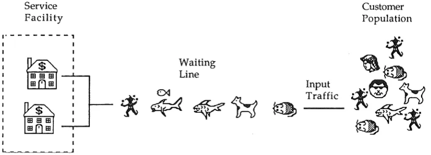
which is the third basic element of any queueing system. Below is a picture of a very simple queueing system:

L

Service Facility

---,

I

Fig. 1 A simple Queueing System

Input Traffic

Customer Population

[image:5.595.65.497.563.719.2]

(6)

6

Population or Source of Customers

The population or source of customer in any queueing system is characterised by the size of it. Some systems are considered to cooperate with a finite population of customers, and others with infinitely large

customer population. We need to clarify that the word

infinite

has a

weaker sense, in that any customer population or source must be finite, but sometimes it is necessary to consider a very large population of customers as an infinite population. This sometimes turns out to be important factor in making the mathematical analysis of queueing system tractable. Finite populations - in modelling internal processes of computer systems. Infinite populations eg. in modelling data communication networks.

Customer Arrivals Pattern

The behaviour of queueing systems depends not only on the size of the population and the rates at which they arrive to the system but also on the pattern that they arrive. Generally, evenly spaced customer arrivals result in better performance of the system, because the service facility can provide a better service. The worst is when customers arrive to the system in clusters, the extreme case of clustered stream of customer arrivals is

sometimes referred to as

batch arrival

pattern.

This project investigates both systems with single customer arrivals and systems with customers arriving in batches. However only exponentially distributed interarrival times are considered here. By exponentially distributed interarrival times we mean that the cumulative distribution function of customer interarrival times is

-At

A[t]

=

1 -

e

₍₁₎

where A the average arrival rate. This arrival pattern possesses the so

called

memoryless property.

If an arrival pattern possesses the memory

less property, the next arrival time is completely independent of the

present or past arrival times, see Allen [4]. Above, we have the symbol A as

the mean rate of customer arrivals, so it is obvious that 1

/A

is the average

interarrival time.

Service Time Distribution.

As mentioned above, this project investigates queueing systems with exponentially and deterministic service times distributions. For the exponential distribution of service times, the memoryless property means that the time remaining to complete the service of a customer is independent of the time already spent in servicing this particular customer. The service time distribution function is given by

(7)

- 1 - e

-t

ws

7

(2)

where µ = 1/Ws, is the average rate at which a server processes customers

when the server is busy

The other service time pattern considered here is deterministic service pattern, where customers require the same service time. The reason why . !b,a.<this service pattern is chosen, is that, it is very common situation in modern data communication systems ie. in transmission of standardised data blocks ( packets of equal size).

Other Relevant Terminologies

Utilisation Coefficient is the term generally used for describing the degree

of utilization of the service facility. It is defined as the proportion of

average arrival rate to the average service rate, and the symbol that is used

for utilisation factor is p. The behaviour of a queueing system is heavily

dependent on the value of utilisation coefficient: the higher the utilisation factor the longer the average delay. Furthermore the level of utilisation affects the probability of buffer overflow.

Average System Delay . The average time the customer spends in the

system, ie. from the arrival time of the customer to J;ke'. its departure, and is defined as ( from Little's formula [3] ), for the exact formula see appendix A (A-1)

Mean number of customers in the system

E[W]

=

-').., ₍₃₎

Average Queue Delay, denoted by the symbol Wq, is the average time that

customer spent in the queue buffer, thus ( for details see appendix A-2)

Mean queue length

E [ W ] =

-q

'A

(4)

Note that the number of customer in the queue is equal to the number of customer in the system minus one, which is the average number of customer in the buffer queue ( for single server queueing system ). From there, using the same reasoning used in Little's formula we can deduce another relation namely : the total average time in the system equals to the average waiting time in queue plus the average service time, which is intuitively clear, ie.

E[W]

=

E[W q] + E[W s] ₍₅₎

i·.

I

i.

(8)

8

This project investigates queueing systems with an assumed infinitely large customer population with poisson arrival pattern, both single and batch arrival case are studied.

Throughout this report we will refer to those queueing systems mentioned above with special kind of notation called Kendall notation, after David Kendall [1], its originator, specially dev;eloped to described queueing systems.

Kendall notation has the form of A/Bl c/K/m/Z, where

A describes the interarrival times distribution of customers

B describes the service time distribution provided by server(s)

c describes the number of servers in the system

K describes the system buffer capacity

m describes the number in the customer population

Z describes the queue discipline used by the system

The symbols used for A and Bin this project are, M stands for exponential interarrival or service time distribution with single arrival or service, M(b)

(9)

9

Chapter Two

The Queue Buffer Capacity.

Basic Assumption

Behaviour of any queueing system depends on the assumed size of the queue buffer in front of the server. Basically there are two options that can be considered: 1) Infinite buffer capacity and 2) Finite buffer capacity.

1) Infinite Buffer Capacity.

Some may argue that there is no buffer of infinite capacity. But the advantage of regarding a buffer as having infinite capacity is the simplicity of analysis. This effect is a consequence of the 'infinite sumability' of many mathematical models of such queueing systems. In many cases, the analysis can result in direct ana~ytical formulas, we need to substitute only numbers to the formulas and get the results by performing simple mathematical computations.

Of course the results produced using such assumption, will only

approximate the behaviour of finite queueing systems. But as will be shown latter, in some particular cases, the approximations are fairly accurate, eg. for low utilisation coefficient and large buffer capacities, the numerical approximations are fairly accurate.

A disadvantage of analysing systems with infinite buffers/ is. that, such

systems are stable only if they are utilised in less than

(!g~?J

thus for

coefficient of utilisation p < 1. The reason for this, is that if we have unlimited buffer capacity and customer arrival rate is higher than the service rate provided by the service facility, then the queue system's buffer capacity will keep growing to an infinitely large size and the system become unstable.

In this project, we analyse the limiting behaviour of stable queueing systems, it is, their behaviour in steady state.

2) Finite Buffer Capacity.

(10)

10

On the other hand, with the analysis of such systems we can obtain exact numerical results with the accuracy being only limited by the precision of the computer used.

What to be Compared

Having considered all the main advantages and disadvantages of both assumptions about the queue system's buffer capacity, we have a question

to ask, what happens if we use numerical results obtained for buffer of

infinite capacity to analyse buffers with a finite capacity. That question summarised the main topic of this project.

To answer that question, first thing that we do is making comparisons on the performance measures of both systems with a certain range of system's buffer capacitys and utilisation.

We compare:

- The probabilities of the system being in a particular states - Average numbers of customers in the systems

- Average of system delays ( mean waiting times)

- The accuracy of approximations used for assessing the buffer overflow probability using numerical results taken from the infinite capacity buffers. .

This project focuses on the last two comparisons, the first two

comparisons are somewhat implied by the last two. If we have high

probability of overflow than it is obvious that we can expect that the probability of large number of customer present in the system must be high. Similarly, the average number of customers in the system and the average system waiting time, this relationship is depicted in equation (3) in the Introduction chapter.

Method of Comparisons

Symbols related to buffers of finite capacity K will be distinguished from

corresponding symbols related to buffers of infinite capacity by subscripts K

and 00, respectively. Thus WK means the delay ( the total time spent in

queue) in a buffer of capacity K, while Woo means the delay on a buffer of

infinite capacity.

(11)

11

The probability that a new customer is not accepted into a system of finite buffer capacity K, shortly, the probability of overflow, can be approximated in two ways:

P' ₁(overflow)

=

P(N 00 ~ K) (6a)

or

P'₂(overflow)

=

P(N00 > K) (6b)

where P(Noo ~ K) is the probability of having Kor more customers in the

queueing system with infinite buffer capacity, and P(Noo > K) is the

probability that there are more than K customers in that system.

A justification for using the former approximation explained above is that,

the event (N(X) ~ K) can be associated with finding the corresponding

queueing system of capacity K full, while P(N(X) > K) can be associated with

the proportion of time when the corresponding queueing system of finite capacity K would be overflowed.

Similarly we formulate two approximations of means delay in finite buffers, by using results obtained for queueing system of infinite buffering capacity:

E' ₁(WK)

=

E(W 00)

*

P(N00 ~ K) (7a)

or

K

L i P(N00

=

i) E'i(WK)

=

_i_=o _ _ _ _ _

11. (1- P'(overflow)] _(7b)

In eq. (7b), either approximation (6a) or (6b) can be used.

The first approximation can be interpreted as the average delay in the infinite buffer system, multiplied by the proportion of time that the ( infinite buffer system finds itself having K or less customers. This ,, approximation, is obtained assuming that, in the steady state theory which .. \ says that, in the steady state, the probability of system being in a particular :

state is the same as the proportion of time that the system is in that '1

particular state.

The second approximation is obtained from the Little's formula for the

average delay in a finite buffer system. The mean queue length is replaced by its approximation (using probabilities of states for infinite buffer system) as well as replacing P(overflow) by its approximation.

(12)

12

Chapter Three

Queueing Systems with Individual Arrivals

All queueing systems in this chapter, are analysed assuming that:

- Customers arrive individually

- Service facility serves one customer after customer following FIFO order - The arrival and departure rates of customers don't change with time and

are independent on the number of customers in the system

- In finite buffer system, customers arriving when the buffer are not accepted to the system and must leave

3.1

M/M/1/oo

and M/M/1/K Queueing Systems Comparison

The first comparison is between M/M/1/oo and M/M/1/K queueing systems. Both queueing system have simple analytical formulas, note that M/M/1/K is the only finite system on which analytical formulas can be obtained.

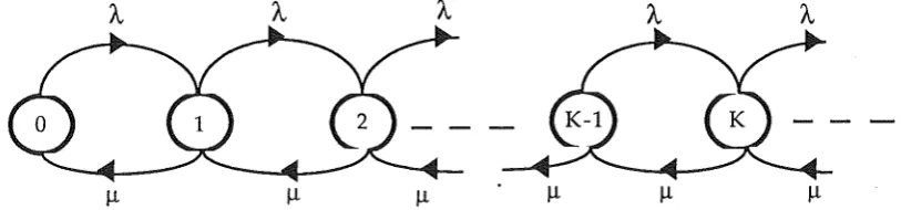
Those simple queueing systems can be analysed using so-called 'birth-and-death' processes. Using this method an arrival of a customer is considered as a birth , while a customer's departure is considered as a death (for derivations of the formulas, discussed in this chapter see [4]).

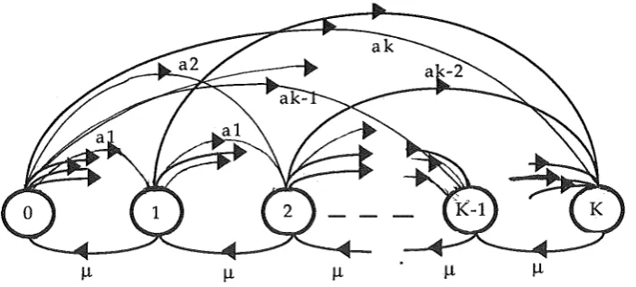
Given the birth rates A and the death rates µ, we have a birth and death

process as described in the diagram below, where each node represents the state of the system ( the number of customers present in the system) :

µ µ µ µ µ µ

Fig. 2-1 Simple Birth-And-Death Process for M/M/1/oo Queueing System

The probability of the infinite buffer system is in state n is

n

P[N00 = n] = (1 - p) p (8)

[image:12.595.63.470.563.658.2]

(13)

n (1 - p) p

K+l

P(NK

=

n)

=

1 -P

1

K+l

13

for tvt= µ

for A=µ

. (9)

where p is the utilisation factor. Thus we get the following two

approximation of P(overflow)

K

P\ (overflow)

=

P(N00 ~ K)

=

P (lOa)

and

K+l

P'₂(overflow)

=

P(N00 > K)

=

p (lOb)

While the average delay for buffer with infinite buffer capacity and buffer with finite capacity, respectively are :

and

p

E[W,,J

=

-(1-p)A

K+l K+l

1 p(l-p )-(K+l)p (1-p)

A K+l K+l

(1-p)(l-p -(1-p)p)

(11)

(12)

Thus E[WK] can be approximated by E'[WK]

=

E[Woo]

*

P[Noo ~ K], which is

equal to

1 p K+l

'\ - (1-p ) /\, 1-p

Comparison Results

/

(13) /

In Fig. 3.1 to Fig. 3.3 we have some graphs showing the comparison

between the exact values of the system waiting time in M/M/1

/K

queueing system and their approximated values obtained from the

formula (13), here we use the average value of service rate

=

1.

It is obvious that as the system's buffer capacity grows, the approximation

(14)

14

But when the (infinite) queueing system are heavily loaded, then this approximation of the average system delay is very inaccurate. For example in fig. 3.2 and K=5, when p = 0.5, then this over-estimation is more than 50% the exact value. But again, as the system's buffer capacity increases this approximation improves, and for K = 100, the approximated values are practically equal to the exact values.

We expect that as the system utilisation gets larger, if the probability of

overflow increases. This happens because, when the rates of arrival get higher, and on average, there would be more customers present in the system, thus the probability of overflow will increase as well.

The probability of overflow approximated by P(Noo ;:::: K) is always bigger

thtin both the exact value P(overflow) and the P(Noo > K) approximation.

In case of P(N= > K) there is a region of p where this probability is smaller

than of P(overflow). Of course, it's highly undesired property of any

approximation of P(overflow), as it could lead to a wrong selection of

system's buffer capacity. However at higher level of utilisation, P(Noo > K) gives values greater than P(overflow) and smaller than P(Noo ;:::: K), thus for higher values of p, P(N= > K) is a better approximation than P(N=;::::

K), because it gives more accurate values, and yet, still with a safety

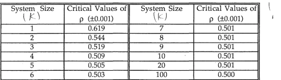
margin. The limit value of p in the region where P(N= ;:::: K) approximates better P(overflow) than P(N=;:::: K) is at about 0.5. The table 3.1 gives that critical values of p separating the region where P(Noo ;:::: K) approximates

P(overflow) better - from the region where P(Noo > K) approximates better.

Table 3.1 The Values of p for that P(N=;:::: K)

=

P(Noo > K) (for M/M/1 Queueing System)

System Size Critical Values of System Size Critical Values of

\ j(J

_p _(±0.001) \ f(:_ J _p _(±0.001)

1 0.619 7 0.501

2 0.544 8 0.501

3 0.519 9 0.501

4 0.509 10 0.501

5 0.505 20 . 0.501

6 0.503 100 0.500

Note that for system's buffer capacity of 1, the crossing point happens when utilisation factor equal to 0.6, this somewhat deviates from the general trend of the crossing point for M/M/1 queueing system, this

behaviour is considered 'normal', because here we have a queueing

system with infinite queue buffer capacity being used to approximate queueing system with no space for queueing at all, so the result of this approximation is irrelevant to our interest.

j

!

J ' , ,

i ''

[image:14.597.63.519.490.620.2]

(15)

2

1.8

1.6

1.4

'2

1.2

"'

,,_,

~ 1

...

(l) O 0.8

0.6

0.4

0.2

0

4

3.5

3

y 2.5

(l)

"'

._,

~ 2

...

(l)

0 1.5

1

0.5

0

.

Mean Waiting Time in M/

Ml

1/ K System

Comparison between

E(WK)

and

E '(WK)

K=l

;

3 K=2

I

'

J 2.5

r

I/

2

y

~

,)'

,,,Y

l /

.;

~ I.,.>"'"

(l)

"'

'-"

~ 1.5 ...

(l) 0

1

,I

'_,,,) ,,,,,,..

c ~ ~ 0.5

~

.,,.

"' "

.

I I I I I 0

0 -

o o o o o o o o o

N ~ ~ ~ ~ ~ 00 ~ - 0 -

o o o o o o o o o

N ~ ~ ~ ~ ~ 00 ~

-Rho ~~~~~- Rho

...__ E' [WK] ....__ E [WK] K=3

5 4.5

4

K=4

:

'

.

,

~

3.5 y

(l) 3

"'

...,

.

'

:

(

~ 2.5

...

(l)

2

0

1.5 1

0.5

0

I

.v

.

1'

/ 17'

:

~

_~

....J ~

L..J

~

...___.

11 r11 11 111 I I I I

.

0

-

N ~

d

~ ~ ~ 00 ~ ...

0 0 0 0 0 0 0 0 0

o o o o o o o o o

- N ~ ~ ~ ~ ~ 00 ~

-Rho Rho

(16)

6

5

4

u

(!)

.;!)

~3

-

(!)

Cl 2

1

0

8

7

6

uS

(!)

"'

._,

~4

-

(!)

Cl 3

2

1

0

Mean Waiting Time in M/

Ml

1/ K System

Comparison between

K=5

... N (') _~Lr)

ci ci ci 0 ci

Rho

K=7

... N (')

"""

Lr)

ci ci ci ci ci Rho

E(WK)

and

E '(WK)

\()

"'

00 0\

ci ci ci ci

\()

"'

00 0\

ci ci ci ci

7 K=6

6

5

u

34

~

a:) 3

Cl 2

1

0

... 0 ... _C'J (') _~Lr) \()

"'

00 0\ ...

ci 0 ci 0 ci ci ci ci ci

Rho

-0- E' [WK]

__._ E [WK]

9

8

7

6

u

] s

~

a:) 4

Cl 3

2

1

0 ...

Graph 3.2

K=8

-

,

:

.

J

:

I

: _I

:

,/

../

-

I /

-/ ti

.

--

_I~~

-

_:

,J

r

-

_~_~

...

-

.

a.JI

'"' 1111 I 111111 I ' I I I I I I I I

0 .--< N C0 -s:t' Lr) \0 !'-. 00 0\ .--<

(17)

u

Q)

$

~

-

Q) 0

10

9

8

7

6

5

4

3

2

1

0

20

18

16

14

6

·4

2

0

Ml

1/ K System

Comparison between

E(W

K)

and

E

'(WK)

K=9

12 K=lO

~

I

10

-1

:

--

I

:

-

u 8

:

)

--.

,

/

-:

-//

Q) tll

...

~ 6

....

_Q)

0

4

:

I ~

,,) ~

-

2

-

_~

..

-

IIIIU

:

-

-"

.

"

.

I I 0

0 - N ~ ~ m ~ ~ 00 ~

-d -d -d -d d d d d d 0

-

d d d N ~ 0 ~ m d d d ~ ~

Rho Rho

K=20 K=lOO

4

.

60

.

50

411

.

I

I//

.

)

v

:

T

.

20

-

.

~

10

... _.. La,A

....---

-

-....

-n

..

...

.

-

_-

.

_"

-·

...

~

- -

...

_{" ' n}

-0

00 ~

-d -d

4

}

...

~

.

-,

....

0 - N ~ ~ m ~ ~ 00 ~ - 0 _{d d d d}- N ~ ~ m _{d d d d d}~ ~ 00 ~

-d -d -d -d d d d d d

Rho Rho

(18)

lxlOO

;::

0

-'-H

~ lxl0-1

>

0

...

0 ' ₀

...

-

...

fJ lxl0-2

,.0

0

I-<

P-<

lxl0-3

0

lxlOO

;:: lxrn-1

0

...

~ lxl0-2

0

...

t,

lxl0-3

...

fJ lxl0-4

,.0

0

~

lxl0-5

lxl0-6

0

Probability of Overflow in M/

Ml

1

I

K

Comparison between

P(overflow), P

_1'

(overflow), P

_{2 '}

(overflow)

lxlOO K=2

;::

o lxl0-1

~ Q)

>

0

...

_e,

lxlff2

...

-...

fJ

,.0

~ lxl0-3

lxl04

... N _C'1 _~II)

'°

t--.. 00

°'

... 0 ... _C'J _C'1 _~II)

'°

ci ci 0 0 ci ci ci ci ci ci 0 0 0 0 ci

Rho

_.__

Rho

P'1(of)

--

P 'iof)

p (of)

lxlOO K=4

lxl0-1

;::

0

~ lxl0-2

Q)

>

O lxl0-3

...

0

;S'

lxl0-4

.

....

fJ

..O lxl0-5

0

~

lxl0-6

lxl0-7

... _C'J (() _~II)

'°

t--.. 00

°'

... 0 ,... _C'J _C'1 ~ II) _'C/

ci 0 ci 0 ci ci ci ci ci ci 0 0 0 0 0

Rho Rho

Graph 3.4

1:.,.

I

t--.. 00

°'

...

ci ci ci

t--.. 00

°'

...

(19)

lxlOO

lxl0- 1

~

..9 lxl0-2

~ _Q)

;> 1x10-3

0

..._,

; 1x10-4

...

~ lxl0-5

~

..c

8 lxl0-6

Po< lxl0-7 lxl0-8 0 lxlOO ! lx10- 1 =

~ lxl0-2

0 _lxl0-3

...

~

lxl0-4

Q) ;>

0 lxl0-5

..._,

i ! !

=

0 _lxl0-6

~

... _lxl0-7

-...

..c _Cll _lxl0-8 ..c lxlff9 0 I-< Po< lxl0-10 l l ! =

-.

~ lxl0-11 lxl0-12 0

Probability of Overflow in M/

Ml

1

I

K

Comparison between

P(overflow), P

1'

(overflow), P

2 '

(overflow)

K=6 K=S

lxlOO

-·

1x10-1

~ lxl0-2

0

]

lxl0-3

i>

lxl0-4

0

..._,

0 _lxl0-5

~

.

.... lxl0-6 ... ... ..c Cll lxl0-7 ..c 0

~ lxl0-8

lxl0-9

lxl0-10

-

N C") ~ iri

'°

['-,, 00 0\ ,...

ci ci 0 0 0 ci ci ci ci

Rho

...

P'1(of)

__._ _P'z(of)

p (of)

K=7

-~

~ ,- lxlOO

lx10-1

~ 1x10-2

o lxl0-3

.~

...-l ~ ,Q Ji,,

II

I

.

I

,... _N C<) _~tr)

ci ci ci 0 ci

Rho

\Cl ['-,, 00 0\

ci ci ci ci ,...

] lxl0-4

O lxl0-5

..._,

; lxlff6

:.:=: lxl0-7

.

...

~ lxl0-8

..c

~ lxl0-9

lxlO-lO

lxl0-11

lxl0-12

Graph3.5

~

-

Ul:il ~

,-! _ j 11'7"'"" ~

~ .___

! _~_~

l

~

v

!

J

'/'

.

fl

'I

lid j

I

•

I •

. .

0 ,... _C'! _C"l ~ iri \0 ['-,, 00 0\ ,...

ci 0 0 0 0 ci ci ci ci

Rho

K=B

..

! _...._,_~r

-I a.,,J _...

-

.----i ~ ~

l _~'fl"

! _cl:₇

! I 'ff

I tfJ

l

If

! I

I

! 4111

! J

,

.

0 ,... N C<) _~_iri

'°

['-,, 00 0\ ,...

ci ci ci 0 0 ci ci ci ci

(20)

lxlOO

lxl0"1

~ lxl0"

2

0 _1x10·3

-~

lxl0"4

(I)

>

0 lxl0·5

...

; lxl0·6

:.:::: 1x10·7

...

, ~ lxl0·8

..0

S lx10·9

p..

~

0

~ (I)

> 0 ... 0 0 ... ... ... ~ ..0 0 H p.. lx10·10 lxl0"11 lx10·12 lxlOO lx10·1 1x10·2 1x10·3 lxl0"4 lxl0·5 lxl0·6 lx10·7 lxl0"8 lxl0"9 1x10·10 lx10·11 lx10·12 ! ! l ! ! = 5 l !

:

Probability of Overflow in M/

Ml

1

I

K

Comparison between

P(overflow), P

1'

(overflow), P

2 '

(overflow)

K=9

-~ ~

-~ ~ i -j ~ ... J ~ ! ~

,;

j/'

f/

II

I O~ lxlOO lxl0"1 lxl0-2 lxl0-3

l

1x10·4

O lxl0·5

...

; lx10"6 :.:::: lxl0"7

~

lxl0"8

..0

S lx10·9

p.. ! l l ! ! l ! ! ! ! K=lO

-A::l ~ ~~

~

.J

v

u

J'

rJ

I!

...

JIJ ~

~ i.,....-

---l

I

lx10·10

lxl0-11

lx10·12

l I

!4'

_,

..

" "

..

0 ,_. N ~ ~ ~ ~ ~ ~ ~ ,_.

O O O O O O O O O

Rho K=20 ~ ! !

*

! !

,

I _JT

i ~

!

,

! _J

!

T

l c 'I

!

J

" "' ,.

..._ P '1(of) _.._ P '2(of) p (of)

-,

lT . . /

lxlOO

lx10·1

~ lxl0"2

O _lx10·3

v

l

1x10·4

O lx10·5

...

; lxl0·6

:.:::: _... lx10"7

~ lx10"8

..0

~ lx10·9

lx10·10

lx10·11

lxl0"12

0 ,_. N ~ ~ ~ ~ ~ 00 ~ ,_.

d d d d d d d d d

Rho

!

,

.

,.

.. ..

_" _"

.

0 ,_. N ~ ~ ~ ~ ~ 00 ~ ,_.

0 0 0 0 0 0 0 0 0

Rho

K= 100

I

.,

I

/

! ) IT/

! / ,J

v

! _cl'/

!

/,,

/

l

/ /

!

I

'/

!

/ /

!

4V/

l 'I'

!

.

0.7 0.75 0.8 0.85 0.9 0.95 1

Rho

(21)

15

3.2 M/D/1/

00

and M/D/1/K Queueing Systems Comparison

These queueing systems need more elaborate analysis. The results could be obtained by means of techniques developed for M/G/1/oo and M/G/1/K queueing system.

The most commonly used method of analysis is known as the 'Embedded Markov Chain' method. Following that we view the system just after every departure (service completion), unlike in case of the birth-and-death model, where we can observe the system at any instant time.

To find the steady state probabilities of an embedded Markov chain, we must solve a set of equations that can be expressed in a matrix form. For example, assuming the system capacity of K :

K

7t = 7t P and

L.,

n.

=

1

i=O 1 ₍₁₄₎

where 7ti is the steady state probability P(N

=

i), n = (1t1, 1t2, 1t3, .... , 7tK), and

P is the transition matrix. A transition matrix is a (KxK) matrix whose

elements, are the probabilities that n customers arrive during one service period, denoted by an's, thus

f

00 -11.t (Att .

an= P[Arrival = n] = e - , - dW₈[t],

n.

0

n= 0, 1, 2 ..

(15)

where W8[t] is the service time distribution, and A is the arrival rates.

Without going further into details of the formulas' derivations, we just

say that the probability of the system being in the state n is 7tn, thus P[N

=

n]

=

7tn, This fact is proven by Gross and Harris [2]. The formulas used to

approximate the probability of overflow are as follows :

and

K-1

P\(overflow) = P(N00~K) = l-L.,P(N00=i)

i=O (16a)

K

P'i(overflow) = P(N00 > K) = 1 -

L.,

P(N00 = i)

i=O (16b)

(22)

16

K

L i P(N00

=

i)

i=O

E'[WK] =

-A(l -P(N00 ~ K)) (17)

and the exact formula for average system delay is

K

L i P(NK

=

i)

i=O

E[WK]

=

-. A [l - P(NK

=

K)] ₍₁₈₎

Comparison Results

The quality of the approximations, can be seen in Fig 3.7 to Fig 3.12, and here we use Ws = 1.

When K (system capacity) = 1, and assuming that the average service rate is 1, the average system waiting times are all equal to one, for all values of utilisation factor (see Fig 3.7, for .K=l). The reason is that, when K=l, we

don't actually have any queue in front of the server, so if a customer

arrives when the service facility is busy, the customer is rejected right

away, and leaves the system. On the other hand, if the service facility is

idle, any new customer is served straight away with a constant service rate equal to 1 (consistent with the assumption above), thus all serviced customers have the average system delay equal to the service rates which is 1.

Figures 3.7 - 3.9 show that the approximation E'[WK] given by Eq.(17) always results in higher values than those produced by the exact formula (18), and we see that as the system's buffer capacity gets larger, again the two curves merge together closer and closer, therefore, the bigger the system's buffer capacity is, the more accurate the approximation is.

For example, for K = 100 (see Fig. 3.9, K=100), all the values of E'[WK] are virtually equal to the exact values. Even when K = 7, for utilisation factor

or p = 0.9, the approximation E'[WK] is only off by 5%, which can be

considered accurate enough, taking into account a usual safety margin.

Comparing the results we obtained for M/M/1 and M/D/1 queueing

systems, we see that for both queueing systems P(Noo ~ K) always produces

greater values P(Noo > K) and the exact values of P(overflow).

Similarly, there is a utilisation region where P(Noo > K) approximation is

better than P(Noo ~ K), by the same reasons as in the case of M/M/1

queueing system. The table below shows us the critical values of p for

applying P(Noo ~ K) and P(Noo > K). For K=100, the crossing point is not displayed on the graph, because the precision used in the computation of

(23)

[image:23.597.61.483.132.260.2]

17

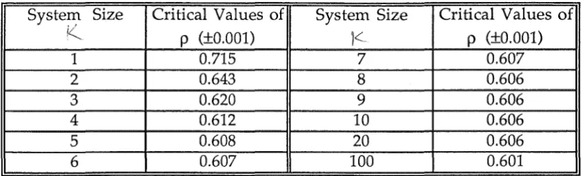
Table 3.2 The Crossing Points Between P(N"" ~ K) and P(N"" > K) Curves for M/D/1 Queueing System

System Size Critical Values of System Size Critical Values of

p (±0.001) j.C p (±0.001)

1 0.715 7 0.607

2 0.643 8 0.606

3 0.620 9 0.606

4 0.612 10 0.606

5 0.608 20 0.606

6 0.607 100 0.601

Conclusion

For single arrival queueing systems, M/M/1 and M/D/1, the

approximations of the average system delay are reasonably good,

especially for queueing system with large buffer capacity.

Approximations of the probability of overflow , P(N"" ~ K) is a better

approximation of P(overflow), than P(Noo > K), for lower utilisation

factors, while for higher utilisation factors the P(N"" > K) approximates better.

i

(24)

1.8

--1.6

-1.4

-

--1.2

-

-Mean Waiting Time in M/

DI

1/K System

Comparison between

E(WK)

and

E'(WK)

K=l

2.5 K=2

.~

.

~ r"'

_ j ₂

-~ ~

- 1

.

_411

~

D"'"'

~

v

_(!)

1 : aJ ~

~ v

] 1.5

$

~

,A

,,,.

-.:!J

~

~ 0.8 0

-

--_A.A

..e,J i...-,.., ~

-.

-

..__.

a.JI

-~

-0

1

0.6

.

--0.4

-

-0.5

-0.2

-

--0

-

I _{I' "}

" " " 0 _" " ,. ,

.. ..

I I I I ·o

-

_N ("! _""! U) \() 1:-,., cq 0\

-

0

-

N C() _""! I.!) \() 1:-,., 00 0\

-d d 0 0 0 d d 0 d _d d d 0 d d d d d

Rho Rho

..._ E' [WK] _.__ E [WK]

K=3 K=4

2.5 3

2 2.5

2

] 1.5

v

(!)

rJl _$

' - '

~ ~ 1.5

-

...

(!)

1 (!)

p p

1

0.5

0 0

0

-

N C() _"Sf' I.!) \() 1:-,., 00 0\

-

0

-

N C() _""! I.!) \() 1:-,., 00 0\

-d d d d d d d d d d d d 0 d d d d d

Rho Rho

Graph3.7

(25)

3.5 3 2.5 ... u Cl) 2 $ ~

~ 1.5

1 0.5 0 4.5 4 3.5 3 1.5 1 0.5 0

DI

1/K System

Comparison between

E(WK)

and

E'(WK)

K=S

4

.

K=6

3.5

3 :

)

!;

~~

"u 2.5 Cl)

"'

' - '

2

.I.I

0

.

-.

.

. .

.

....

.

11 111

0

~

...

Cl) 0 1.5

.

l"

:

- ~

u.,J ~ t '

.

-·

1

-.

0.5

.

-.

0 I I l l II J ffJ I H I ·1m I I I 111

,-< N M

"""

LI)

'°

d d d d d d

Rho K=7 - ~ !)I' ~ ~ ~ ..,.j t--. d J ~

00 O'\ ,-< 0

d d

..._ E' [WK] _._ E [WK]

'

!;

5 4.5 4 3.5 :

_) 'I

~

] 3

$

~2.5

~

2

: '

.

:

.

-

-; :

I II I 11 II I II II II II Ill II [III I j I II I II I

1.5

1

0.5

0 I 111

,-< N M _~LI)

'°

t--. 00 O'\ ,-< 0

d d d 0 _d _d _d d d

Rho

Graph3.8

,-< N M _~ LI)

'°

t--. 00 O'\ ,-<

d d d 0 _d _d _d d d

Rho K=B

'

'/;

(/

,J

·'

JI!'

.) I.JI!'

La.,

w

...

-·

11 II I I l l II II II 111 I I II II

,-< N M _~ ₁₁₁

'°

t--. 00 O'\ ,-<

d d d 0 0 d d d d

Rho

(26)

6

5

4

2

1

0

12

10

8

u (lJ

::!:,

~ 6

... (lJ

0

4

2

0

.

-.

-0

.

-.

.

DI

1/K System

Comparison between

--

-"

-

N

0 0

-- --

-

-' " I-'

K=9

~

E(WK)

and

E'(WK)

1

j'

,,

I

JI

,

1,.-1""

u

_(lJ

::!:,

~ 3 -J---4--1---4---4--+-_....--l~"""""_....--I

-

(lJ

0

2-J---4~-1---4---4~-+-_...,.c:i~-4-_....--1

.a.J ~

..

"' I I

('(') _"<:!' tr) \() t--. 00 0\

-

0

-

N ('(')

"""' tr) \() t--. 00 0\

-0 0 0 0 0 0 0 0 0 0 0 0 0 0 0 0

Rho Rho

_._ E' [WK]

__._ E [WK]

K=20

35 K= 100 411 30

.

)

25

.

1

.

)

l

-' ~

c

.

I

10

.A-I ~

--

'

.

-·

A,J ~

5

...

-

-I

" 0 I I II 11 II I ·1 H I II I I I I I I I I

.

0 ..-< N ('(') "<:!' t.n \D t--. 00 0\ r l

o o o o o o o o o

0 ,-, N ('(') """' t.n \D t--. 00 0\ ,-,

o o o o o o o o o

Rho Rho

(27)

lxlOO

~

0

-1J

_;:,. 1x10·1 0

...

0

...

-...

~ lx10·2

..0

0

H

p...

lx10·3

0

lxlOO

1x10·1

~

0

q3 lx10·2

(I)

;:,. O lxl0"3 ...

0

.£

lx10·4

...

..0 <Ii ..O lx10"5

0

H

p...

lxl0·6

lx10·7

0

Probability of Overflow in

Ml DI

1

I

K

Comparison between

P(overflow), P

_1'

(overflow), P

_{2 '}

(overflow)

lxlOO K=2

~ lxl0"1

0

tE

(I)

;:,.

O lx10·2

...

0 0

S

lxl0"3

~

..0 0

&:: lxl0·4

lx10"5

-

N ('() _~If') _"I t-.. 00 0\

-

0

-

C',J ("/ ~ If') "I t-.. ci ci ci 0 0 0 ci ci ci ci 0 0 0 0 0 ci

Rho

...__

Rho

P'1(of)

..._

P 'iof)

P (of)

K=3 K=4

cq 0\

0 ci

lxlOO

lx10·1 ~ ~

,...

~

6

lx10·2

] lxl0"3

8

lx10·4

0

E

1x10·5

...

.

...

~ lxl0·6

..0

0

rt

lxlff7

lxl0·8

lxl0·9

!

--

,.

-

,...

- j ~

~~

I

,

~

,,

!

4,,

/

1

,.

/

!

; I

.

! 4 I

I

!

I

; I

"'

....

"

. .

-""

-

N M _~If') \() t-.. 00 0\

-ci -ci -ci -ci 0 -ci ci ci ci ci ci ci ci ci N M ~ ~ \0 t-.. 00 0\ -ci -ci -ci 0 0

Rho Rho

(28)

lxlOO

lxl0- 1

~ lx10-2

o lxl0-3

1

lxl0-4

O lxl0-5

'I-<

.e,

lxl0-6

:..:::1 lxl0-7

~ lxl0-8

,.a

o lxl0-9

~ lxlO-IO lxl0-11 lxl0-12 lxlOO lxlO-l

~ lxl0-2

o lxl0-3

] lxl0-4

;;.

0 lxl0-5

'I-<

_e,

lxl0-6

:..:::1 lxl0-7

~ lxl0-8

,.a

8 lxl0-9

~

lxlO-IO

lxl0- 11 lxl0-12

Probability of Overflow in M/

DI

1

I

K

Comparison between

P(overflow), Pi' (overfJow), P/ (overflow)

K=S

...

~ _-

.

~

-! IIIY ~ i

-! ~ ~

! _~7

! _IT!

v

~ ,I

I/'

I

J)

!

I

!•

=

I

i ,I

!

II II I' I I'" I I I I I

...

1111 I I I I

...

I " 0 - N ~ ~ ~ ~ ~ ~ ~

-0 -0 -0 -0 -0 -0 -0 0 0

Rho

K=7

..

! _...J_~

! ~ i..,...,,,"'

! - 4 ~ ...

! A/. ~

! _{j ~}

l

11/

i T;'

!

YI

!

,~

:

•' I

l

I

! I

II I 111 I II I 11 II I I I

"' _" 0 - ~ ~ ~ ~ ~ ~ 00 ~

-0 0 0 0 0 0 0 0 0

Rho

lxlOO

lxl0- 1

~ lx10-2

0 _lxl0-3

tS

(U _lxl0-4

;;.

0 lxl0-5

'I-< 0 lxl0-6 ~ lx10-7 ... ... ... ~ ,.a 0 ~ O ~ lxl0-8 lxlff9 lxlO-!O lxl0-11 lxl0-12 P'1(of) P 'iof)

p (of)

lxlOO

lxl0-1

lxl0-2

lxl0-3

1

lxl0-4

O lxl0-5

'I-<

.e,

lxl0-6

:..:::1 lxl0-7

~

lxl0-8

,.a

~ lxl0-9

lxlO-IO

lxl0-11 lxl0-12

Graph 3.11

K=6

-! _{. ..J}~

:

..) ~

--

-l ~ :;.,""

! I ~

,

!

,n

,,,

: _ITJ/

l _)

'/

!

r,

!

~,

= /, I

,.

!

II U I I II

....

I I I I I I I I I " I I I I I

....

I I I I 0 ₀- ~ ~ ~ ~ ~ ~ 00 ~

-0 0 0 0 0 0 0 0

Rho

K=8

-! _-J._~

! ~ Ji'_.... ~

! ~ ~

!

.~

,,

! JIJ, 7

I ,J

v

i

J~/

!

,,

"

! i'f

!

,1,

!

II

! 4

"

.

1111

0 - ~ ~ ~ ~ ~ ~ 00 ~

-0 0 0 0 0 0 0 0 0

(29)

lxlOO 1x10-l

~ lxl0-2

0 _lxl0-3

...

't1 (1) _lxl0-4

>

0 lxl0-5

'+<

.e-,

lxl0-6

;.:: lxl0-7

~ lxl0-8

.n

e

1x10-9 ~ lxl0-10 lxl0-11 lxl0-12 lxlOO lxl0-1

~ lx10-2

o lxl0-3

~

(1) lxl0-4

>

O lxl0-5

'+<

.e-,

lxl0-6

;.:: lxl0-7

~ lxl0-8

.n

e

1x10-9

~ lxlO-IO lxl0-11 lxl0-12 ! = ! ! ! : ! ~ ~ ! l !

Probability of Overflow in M/

DI

1

I

K

Comparison between

P(overflow), Pi' (overflow),

Pi'

(overflow)

K=9

-

K=10

_ j

r

!

---

"

...

--

l

. J g;.-' l

-.,

I ~

,,,,,--~

,,,-..,/ P"'

lxlOO lxl0-1

~ lx10-2

o lxl0-3

~ _~

lxl0-4

~--J~

,;;

,,,

,,

J~

yj

4'1/

J,11

....

" I I

"

O lxl0-5

'+<

.e-,

lxl0-6

;.:: lxl0-7

...

~ lxl0-8

.n

8 1x10-9

~

lxlO-lO

lxl0-11 1x10-12

! _~

I ~ :I'

! l

PY

! _T)

! _~

r.t

!

,J

l

• 'f

! I

"' I

..

"

0 - N ~ ~ ~ ~ ~ 00 ~

-ci -ci ci ci ci ci ci ci ci 0 - N ~ ~ ~ ~ ~ 00 ~

-0 -0 -0 -0 -0 -0 -0 -0 0

Rho K=20 ~ ! ! l

! '111

!

rl

1

""

l

II

! _~

!

"JI

l

,

I

J

" 1•

...._ p '1(of)

_._ P 'iof)

P (of)

"'

lxlOO

,f ~ lx10-1

"'

/ ~ lxl0-2

0

(/ ... 't1 ₍₁₎ lxlff3

>

lxl0-4

0

'+<

0 _1x10-5

.0 ... lxl0-6 ... ... ~ lx10-7 .n 0

&:: lxl0-8

lxlff9

.

lxl0-10

0 - N ~ ~ ~ ~ ~ 00 ~

-ci -ci -ci ci ci ci ci ci ci

Rho Graph3.12 Rho K=lOO =

.

•

i

I

!

I

,

!

, If

' J

!

,

/

l

' I

!

//

!

j

I

!

/1

!

v

...

00 N ~ ~ 00 ~ N ~ ~ 00

-ci 00 ~ ~ ~ ci ~ ~ ~ ~

0 0 0 0 0 0 0 0

(30)

18

Chapter Four

Queueing Systems with Batched Arrivals

If we the assumption that customers arrive individually, then we have the

M(b) /M/1 queueing system. In this queueing system, we still have Poisson

arrival stream, but the difference is that ; the of customers arrive in random groups (batches), ie. more than one customer can arrive at the same instant of time.

The state diagram for this system is depicted below :

µ µ µ µ µ

Fig 4.1 State transition diagram for M(b) /M/1/K queueing system

In the queueing systems with individual arrivals the transitions are only allowed to the nearest neighbours, for example from state 4 we can have a transition to state 5 or state 3, but not to, say, state 10.

On the other hand, in queueing systems with batched arrivals, multi-step transitions occur whenever batches of more than one customer arrive. The size of an arriving batch can take any positive integer value, and we

assume that the batch size

i

occurs with the probability ai,

From the state transition diagram above, we can derive balance equations that imply the 'flow conservation' principle, see Gross and Harris [2].

Following that principle, for system with finite buffer capacity, we have balance equations as follows :

K-n n

P[NK

=

n] (µ+La)

=

P[NK

=

n+l] µ

+

LP[NK

=

n-j] a.

. 1 . 1 J

[image:30.595.106.458.315.474.2]

(31)

and since

thus

K

P[NK=O]L,.ai = µP[NK=l]

i=l

K

P[NK

=

OJ

L,.

ai

i=l

P[NK

=

l]

=

-µ

19

(20)

(21)

where ai is assumed to be from geometric distribution, thus ai

=

(1 - q) qi-1

for (0 < q < 1).

Each of the probabilities P[N

=

n] can be computed recursively starting

from N

=

0, then working all the way up from N

=

0 to K.

The calculation of the average system response is still using the same method as previously done for the M/D/1 queueing system ( based on Little's formula). However the calculation of the probability of overflow is

more complicated than as it w·as before for queueing systems with

individual arrivals. Let us note that overflow can happen even in the state 0, if more than Knew customers arrive. plus the probability of state 1 and 1 or more customers arrive. In state 1 overflow happens if more than K-l customers arrive, etc. The exact formuK-la for the probabiK-lity of overfK-low, and its approximations are listed in the Appendix A-3.

The Comparison

The comparison is done for three different value of

q

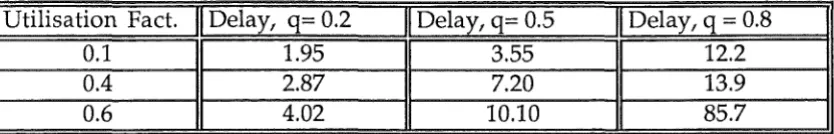
(parameter for the

geometric distribution of the batch size ), namely 0.2, 0.5, 0.8, what corresponds to the average batch sizes of 5, 2, 1.25. The results are shown in Fig. 4.1 to 4.18.

It is noticeable, that the curve for E'[Woo] in every case where system's

buffer capacity is 1, is missing. This effect is caused by the fact that P'(overflow)

=

1 for all values of utilisation factor p and

q,

and we try to approximate a queueing system with no queue buffer capacity, with a queueing system with unlimited buffer capacity.

Looking at the graph for mean system's waiting time, we don't see any

significant difference, for various q values except that the waiting time is

higher when q is bigger ( see graph 4.1, 4.2, 4.3 ), as an example, see the table

(32)

20

Table 4.1 The effect of average batch size to the average system waiting time ( in secs. )

Utilisation Fact.

II

Delay, q= 0.2 Delay, q= 0.5 Delay, q = 0.8

0.1 1.95 3.55 12.2

0.4 2.87 7.20 13.9

0.6 4.02 10.10 85.7

If we look at the values of P'1 (overflow) and P'2(overflow), we see that

again P(Noo 2 K) is always bigger than both the P(Noo > K) and the exact

value, but this time the P(Noo > K) curve never crosses the P(Noo 2 K)

curve. In fact for q = 0.8, the P(Noo 2 K) is under P(overflow) curve. That

fact makes us able to conclude that for the batched arrival case of M(b) /M/1

queueing system, P(Noo 2 K) is the better approximation of P(overflow).

Conclusion.

The average batch size of arrivals effects the performance of queueing system, in such a way, that the sp.1aller the average batch size, the shorter the average system waiting time.

Another observation is that P(Noo 2 K) is better approximation of the exact

[image:32.597.67.484.119.186.2]

(33)

100

CJ

(lJ

"'

' - '

~

... (lJ

p 10

1

0 ...

ci

1000

100

CJ

(lJ

"'

._, ~ ...

(lJ

p 10

1

0 ...

ci

Mean Waiting Time in

Mb/MI 1

I

K

Comparison Between

E(W K)

and

E '(WK)

q

=

0. 2

100

CJ _(lJ

"'

--

_~

...

(lJ

p 10

1

N <:<") "<:!' II) \0 I:'-... 00 0\ ... 0 ... N <:<") _"<!! II)

ci ci ci ci ci ci ci ci ci ci ci 0 ci

Rho

_._ E' [WK] Rho

_._ E [WK]

K=3 K=4

1000

100

--

v (lJ

"'

._..

~

-

(lJ

p 10

1

N <:<") "<:!' II) \0 I:'-... 00 0\ ... 0 ... N <:<") _"<!! If)

ci ci ci ci ci ci ci ci ci ci ci 0 ci

Rho Rho

Graph 4.1

\0 I:'-...

ci ci

\0 I:'-...

ci ci

00 0\

ci ci

00 0\

ci ci

-...

(34)

100

v Q)

$

~

-

Q) 0

10

1

0

-

_C'-!

ci 0

1000

100

v

_Q)

$

~

-

Q) 0

10

1

0

-

N

d d

Mean Waiting Time in

Mb)

M

I

1

I

K

Comparison Between

E(W0

and

E

'(WK)

q

=

0. 5

K=2

100

v Q)

$

~ ...

Q) 0

10

1

<:') _~_Lr'l \0 [:-,.. 00 0\

-

0

-

N <:') ~ I.I") \0

0 0 0 d d d d d d 0 0 _d d

Rho

-e-

E' [WK] Rho

...._.. E [WK]

K=3 K=4

1000

100 'u

Q) <I)

'-"

~

-

Q) 0

10

1

('() _~_Lr'l \0 [:-,.. 00 0\

-

0

-

N ('() _~I.I") \0

d 0 0 d d d d d d d 0 _d _d

Rho Rho

Graph4.2

[:-,.. 00 0\

-d d d

[:-,.. 00 0\

(35)

10000

1000

u

QJ

CJ) ...,

~ 100

...

QJ

p

10

1

10000

1000

u

_QJ

CJ)

._,,

~ 100

... QJ 0

10

1

:

.

:

.

:

-=

:

I 111 I II I

Mb)

M

I

1

I

K

Comparison Between

E(W

K)

and

E

'(WK)

q

=

0. 8

K=l K=2

•

I

j

_u 1000

./

!..-'

.,,,,,

...

---

....-

~

QJ

CJ)

'-"

~ 100

...

QJ

0

10

I II I II II II II I' II I I I 11111 1111 II II

0 ... N C1') _"1! LI")

'°

[:-... 00

°'

... 0 ... N C1') _"1! LI")

'°

ci ci ci 0 _{ci ci ci ci ci} _{ci ci ci} 0 _{ci ci}

Rho

..._ E' [WK] Rho

....__ E [WK] K=3

:

c

.

A

:

'

I

.

~ ....

,

: _a....l

.

--

...

-1000

u

_QJ

.!!J,

~ 100

...

QJ

.

--

0

: 10

I 111 I II I 11 II I II II 1111 ,II II 1111 j l l l I 111 I II II

[:-... 00

°'

... ci ci ci

0 ,.... N C<"J ~ LI") \0 t--. 00 0\ .-<

ci ci ci ci ci ci ci ci ci 0 ci ci ci ci ci ci ci ci ci .-< N C<"J ~ LI") \0 t--. 00 0\ .-<

Rho Rho

(36)

100

u

(1)

"'

._,

1?

...

(1) p

10

1

1000

100

u

(1)

$

1?

-

(1) p

10

0 ... N

ci ci

Mb/

M

I

1

I

K

Comparison Between

E(W

0

and

E '(WK)

q

=

0. 2

K=5 K=6

100

u ₍₁₎

"'

._,

1?

...

(1) p

10

1

r0 'Cf< L{) \0 t.... co 0\ ... 0 ... N r0 'Cf< L{) \0

ci ci _ci ci ci ci ci _{ci ci} ci ci _{ci ci}

Rho

...__ E' [WK] Rho

__..__ E [WK]

K=7 K=B

1000

100

--

u (1)

"'

._.

1?

-

(1) p

10

t.... co 0\ ...

ci ci ci

0 ,-, N r0 'Cf< L{) \0 t.... CO 0\ ,-;

ci ci ci ci ci ci ci ci ci 0 ci ci ci ,-; N r0 ci 'Cf< ci ci ci L{) \0 t.... CO ci ci 0\ ,-,

Rho Rho

(37)

100

u

QJ

-3

~

... QJ Cl

10

1

1000

100

u

QJ

-3

~

... QJ Cl

10

0 ... N

c:i c:i

Mean Waiting Time in

Mb)

MI

1

I

K

Comparison Between

E(WJ and E '(WK)

q

=

0. 5

K=S K=6

100

u

QJ

tll .._, ~

...

QJ

Cl

10

1

C<) '<t' l() \0 r:,... 00 0\ ... 0 ... N C<) _~l() \0

c:i c:i d c:i d c:i c:i d c:i c:i 0 c:i d

Rho Rho

..._ E' [WK]

_.__ E [WK]

K=7 K=B

1000

100

u _QJ -3

~

... QJ

0

10

r:,... 00 0\ ...

d c:i c:i

0 ,... N C0 '<t' l() \0 r:,... 00 0\ ,-<

d d d d d c:i d c:i d 0 d ,... N c:i C0 d d '<t' d d d d d l() \0 r:,... 00 0\ ,...

Rho Rho

(38)

1000

CJ

Q)

en

._.,

~ 100

...

Q) 0

10

10000 ;

--.

-1000 §

--CJ

-Q)

-en

.._.

~

~ 100

...

Q)

0

-

_...

-10 :

:

1

.

,

.

0 ... N

d d

Mb)

M

I

1

I

K

Comparison Between

E(W

0

and

E '(WK)

q

=

0. 8

K=5 K=6

10000 :

.

1000

~

CJ

Q)

..!!:,

~ 100

-

Q)

:

~ ~

-

___.

0

....

-

-.

10

1

.

1

" o I I I

. ..

""" U") \() ['...

d d d d 0 -.::t: Lr) 0 "? 0

Rho Rho

K=7 K=8

10000 :

.

J

I

~

,,,,,...

-1000

CJ Q)

en

...

~ 100

...

Q)

.

;

.

: _-A

...

:

0

.

-"""'

10 : :

"

.

" ,

..

1 ,

.

C() U") \() ['... 00

°'

... 0 ... N C() U") \() ['...

J

t

~

,.)

"

J

I

~

,.,J

.

00

°'

...

-.::t: -.::t:

d 0 _d _d d d d d d d 0 d d d d d

Rho Rho

Graph4.6

! ,

(39)

100

u

(I)

-!!)

~

-

(I)

0

10

1

0

-

N

ci ci

1000

100

u

_(I)

"'

._,

~

-

(I)

0

10

1

0

-

N

ci ci

Mb)

MI

1

I

K

Comparison Between

E(W0

and

E '(WK)

q

=

0. 2

K=9 K=lO

100

u

(I)

"'

'-"

~

-

(I)

0

10

1

c-0 _~II) \0 t-,., 00 ~ ... 0

-

N c-0 'tj< II) \0 ci 0 ci ci ci ci ci ci ci ci ci ci ci

Rho Rho

...._ E' [WK]

_.__ E [WK]

K=20 K=lOO

1000

100

u

QJ

"'

--

_~

-

(I)

0

10

1

c-0 'tj< II) \0 t--.. 00 ~ ... 0 ... N c-0 'tj< Lt) \0 ci ci ci ci ci ci ci ci ci ci ci ci ci

Rho Rho

Graph4.7

t--.. 00 ~

-ci -ci -ci

t--.. 00 ~

(40)

u

_Q)

r.r,

._, ~

-

Q)

0

u Q)

r.r,

.._, ~

-

Q)

0 100

10

1

0 ... N

c:5 c:5

Mb)

M

I

1

I

K

Comparison Between

E(W

0

and

E

'(WK)

q

=

0. 5

K=9 K=lO

100

u

_Q)

$

~

-

Q)

0

10

1

('() _"<!! L!")

"'

t-.. 00

°'

... 0 ... N ('() _"<!! L!")

"'

c:5 0 c:5 c:5 c:5 c:5 c:5 c:5 c:5 c:5 0 c:5 c:5

Rho Rho

K= 100 K=20

1000...--,.~.--....--,---,,---,--,--,..~.--~

100 100

~ ...

Q)

0

10 10

1 1

0

-

N ('() 'tj' L!")

"'

!:--. 00

°'

-

0

-

N ('() _"<!! L!")

"'

!:--.

c:5 c:5 c:5 c:5 c:5 c:5 c:5 c:5 c:5 c:5 c:5 c:

Queueing Models With Finite and Infinite Buffering Capacity : A Comparative Study