Performance Analysis of Two Priority Queuing Systems in
Tandem
Faouzi Kamoun
College of Technological Innovation, Zayed University, Dubai, UAE Email: [email protected]
Received September 19, 2012; revised October 22, 2012; accepted November 2, 2012
ABSTRACT
In this paper, we consider a tandem of two head-of-line (HOL) non-preemptive priority queuing systems, each with a single server and a deterministic service-time. Two classes of traffic are considered, namely high priority and low prior- ity traffic. By means of a generating function approach, we present a technique to derive closed-form expressions for the mean buffer occupancy at each node and mean delay. Finally, we illustrate our solution technique with some nu- merical examples, whereby we illustrate the starvation impact of the HOL priority scheduling discipline on the per- formance of the low-priority traffic stream. Our research highlights the important fact that the unfairness of the HOL priority scheduling becomes even more noticeable at the network level. Thus this priority mechanism should be used with caution.
Keywords: Priority Queuing System; Tandem Queues; Performance Analysis; Discrete-Time Queues
1. Introduction
In this contribution, we consider two discrete-time prior- ity queuing systems (hereafter referred to as PQS1 and PQS2) in tandem. Each PQS implements a non-preemp- tive head-of-line (HOL) priority scheduling with a single server. We consider two types of priority customers, namely high-priority and low priority customers (hereaf- ter referred to as class-1 and class-2, respectively). The number of class-1 and class-2 arrivals within a slot can be correlated random variables.
The main thrust behind our interest to explore the per- formance of tandem priority queues is that previous studies have focused on an isolated priority queuing sys- tem. However, it is well known that in a typical (store and forward) network environment, customers go through a number of switching nodes before reaching their final destinations. For instance, customers belonging to a vir- tual connection are stored and forwarded through a num- ber of queues in tandem. Similarly, in many manufactur- ing and service applications (including health-care and banking), customers (or jobs) need to go through a num- ber of prioritized service facilities before completing a single transaction. At the same time, none of the previous studies on tandem queues have considered multi-class priority scheduling schemes. It is well known however that next generation telecommunications networks are being built around the inspiration of having a single cost- effective packet-based network that is capable of sup-
porting diverse classes of services, each with its own Quality of Service (QoS) requirement. For instance, real- time traffic is delay and delay-jitter sensitive, while non- real-time applications are mainly loss sensitive. To achieve this goal, various packet service disciplines that deter- mine the order by which customers are served have been proposed. Among the simplest time-priority scheduling schemes, the non-preemptive head-of-line (HOL) priority scheduling discipline has been proposed to provide dif- ferentiated services to the high-priority traffic class. Un- der this scheme, the server always schedules the delay- sensitive traffic first (if present). Many previous studies (see for example [1-4]) have analyzed the performance of discrete-time HOL-priority queuing systems (in terms of system content and/or customer delay) under various assumptions regarding the arrival and service time dis- tributions. In particular, Walraevens et al. [5] analyzed a single server discrete-time HOL priority queuing system in steady-state. The corresponding transient results were reported in [6], while the case of multi-server HOL prior- ity queue is treated in [7]. In [8], Walraevens et al. ana- lyzed the busy periods and the output characteristics of a HOL priority queue. Kamoun [9] analyzed a HOL prior- ity queuing system which is subjected to a Markovian interruption process. However, to our best knowledge, none of the previous contributions addressed the case where customers have to go through more than one pri- ority queuing stage.
queuing model being considered, the solution technique being developed to extract explicit expressions for the various performance measures, and the new insights pro- vided on the performance of HOL priority queuing sys- tems in a small “network” environment:
First, we add to the existing literature on non-preemp- tive priority models by considering two priority-based queuing systems in tandem. This tandem configuration of two PQS stages makes the resulting model more practical and flexible in studying more realistic priority-based queuing systems.
Second, we demonstrate how a generating function can be used to derive closed-form expressions for the mean buffer occupancies and mean delays. The closed- form expressions of these performance measures make it very convenient to understand the effect of various sys- tem parameters on the performance of both traffic types. In particular, this research demonstrates how the starva- tion of the low-priority traffic, due to the HOL priority scheduling discipline, is particularly accentuated at the second stage. Our approach also bypasses the need to characterize or approximate the output process of the first PQS stage. Last, the exact expressions for some key performance measures can also be used as baselines to validate the accuracy of potential approximation tech- niques.
The remainder of this paper is organized as follows: In Sections 2 and 3, we describe the queuing model and derive an expression for the Joint Probability Generating Function (JPGF) of the system state vector. In Section 4, we derive explicit expressions for some boundary terms appearing in the JPGF. From this JPGF, the marginal PGFs of the system contents at three of the four nodes, as well as several other JPGFs are derived, as illustrated in Section 5. Closed-form expressions for the first moments of the system contents and customer delay are presented in Section 6. Numerical results that provide insights into the behavior of the queuing model are provided in Sec- tion 7. In particular, we wanted to further explore the impact of the HOL priority scheduling discipline in a tandem configuration on the performance of class-1 and class-2 customers. Finally, a summary of the main find- ings of the papers and some suggestions for further re- search are provided in Section 8.
2. Analytical Model Description
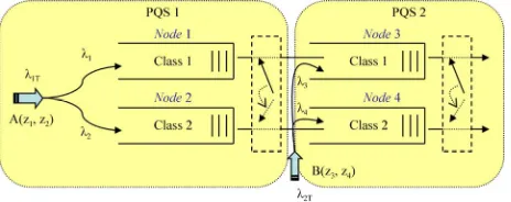
We consider two discrete-time priority queuing systems (PQS) in a tandem configuration. Each PQS has an infinite storage capacity and a single (FCFS) server. The time axis is divided into equal length slots and customer service completion is synchronized to occur at the slot boundaries. Here a slot is the time period required to transmit exactly one customer from the system. It is
assumed that a customer which arrives during a slot cannot be served before the beginning of the next slot. A “conceptual” diagram for our queuing model is depicted in Figure 1.
As shown in Figure 1, in each PQS, customers are served based on a HOL time-priority scheme, whereby type-1 customers have absolute non-preemptive priority over type-2 customers. Under this priority scheme, the server will always serve type-1 customers (if any). If there are no type-1 customers, then type-2 customers (if any) will be served. The model shown in Figure 1 can be viewed as two HOL priority queuing systems cascaded in tandem (PQS1 and PQS 2), or as two parallel tandem queuing systems, which are coupled. In the latter case, the first tandem system consist of two high-priority queues (nodes 1 and 3), while the second system consists of the two low-priority queues (nodes 2 and 4). We also note that the input to the high/low priority queues (node 3/4 in PQS 2) consists of new type 1/2 customers joining the network (exogenous arrivals), as well as type 1/2 cus- tomers which completed service at the first PQS. It is also clear from the model description that the high-pri- ority traffic stream, traversing nodes 1 and 3, is not in- terrupted by the HOL priority scheduling mechanism. The low-priority traffic stream, on the other hand, is subjected to two interruptions, at nodes 2 and 4. It is also assumed that inter-stage departures are not allowed.
In the sequel, we denote the number of arrivals of class-j customers to PQS 1 during slot k by j k,
. These arrivals constitute a series of i.i.d. random vari- ables with the common joint probability generating func-tion 1 2 1 2
1, 2
a j
,
a1,k a2,kA z z E z z , independent of k. We
define the marginal pgfs of the arrivals to PQS 1 from class-1 and class-2 customers during a slot by
1,1 1 1
k
a
A z E z
2,2 2 2
k
a
A z E z
1A
and
respectively.
The marginal arrival rates of class-j (j = 1, 2) to PQS 1 are denoted by j j . We further denote the total
number of arriving customers to PQS 1 during slot kby
1 ,T k 1,k 2,k
a a a , with corresponding pgf AT z
1T AT 1 1 2
. The total arrival rate to PQS 1 is denoted
[image:2.595.309.541.617.709.2] . Similarly, we denote the number
of “exogenous” arrivals of class-j customers to PQS 2 during slot k by j k, . These arrivals constitute a series of i.i.d. random variables with the common joint probability generating function 3 4 , independent of k. We define the marginal pgfs of the exogenous arrivals to PQS 2 from class-1 and class-2
customers during a slot by and
respectively.
1, 2
b j1,k 2,k
b b
E z z
1, 3
k
b E z
1 3, 4
B j
b
3, 4
B z z
3 3B z
2,4 4 4
k
b
B z E z
The marginal exogenous arrival rates of class-j (j = 1,
2) to PQS 2 are denoted by j j . We
further denote the total number of exogenous arrivals to PQS 2 during slot k by 2 ,T k 1,k 2,k, with corre-
sponding pgf
b b
T
B z
2T BT 1 3. The total arrival rate to PQS 2 is denoted by 4. The total arrival rate to the whole system is denoted by
1
1T AT BT 1 2 3 4
, ,u ,u
u
.
In the sequel, we assume that the system is stable and that a stochastic equilibrium exists.
Our model allows for the number of class-1 and class-2 arrivals to each PQS, within a slot, to be corre- lated random variables. This type of correlation can oc- cur for instance when an incoming job (customer) can be split into two parts, an urgent and a non-urgent part, where the urgent part is of class-1, while the non-urgent part is of class-2. Taking into account this correlation in the arrival process leads to more accurate performance results [10]. In the next sections, we will demonstrate that an analysis based on probability generating functions approach can be used to derive some relevant perform- ance measures for the queuing system under considera- tion.
3. Mathematical Model
The queuing model, shown in Figure 1, can be formu- lated as a discrete-time multidimensional Markov chain. The state of the system is defined by 1,k 2,k 3,k 4,k
where i k, is the system content of node i (i = 1 - 4) at
the end of the kth slot. The evolution of the system con- tents is described by the following system equations:
u u
2, 1,
2, 1,
1, 1 1, 1, 1
2, 2, 1
2, 1
2, 2, 1
3, 1 3, 1, 1 1,
4, 2, 1 0 0
4, 1
4, 2, 1 2, 1 0 0
1
1
1 1
k k
k k
k k k
k k
k
k k
k k k k
k k u
k
k k k u u
u u a
u a
u
u a
u u b u
u b
u
u b b
1, 1,
3,
1 if 0
if 0
if 0
1 if
k k
u k
u
u
u
3,k 0
u
(1)
where x is a binary-valued random variable which takes the value 1 if x > 0 and 0 otherwise, while 1x is
the indicator function which takes the value 1 if x is true and 0 otherwise.
The first two expressions in (1) follow from the fact that high priority customers are not in influenced by low-priority customers, while a low priority customer can only be served, if there are no high priority custom- ers in PQS1 (which leads to the second equation). The last two expressions in (1) follow from similar arguments, in addition to taking into account the fact that the output of high/low priority queue in PQS1 (if any) will also constitute an input to the high/low priority queue in PQS2. We also took into account the fact that the low- priority node (2) can only forward a customer to the downstream low-priority node (3) if it is not empty and if the there are no high priority customers in PQS1.
Next, define the JPGF of system contents at the end of the kth slot as follows:
1, 2, 3, 4,
1 2 3 4 1 2 3 4
1 2 3 4 0 0 0 0
, , ,
, , ,
k k k k
u u u u
k
i j k l
k
i j k l
Q z z z z E z z z z
z z z z p i j k l
(2)where
, , ,
1, , 2, , 3, , 4,k k k k k
p i j k l pr u i u j u k u l
1, 1 2, 1 3, 1 4, 1 1 1, 2, 3, 4 1 2 3 4 .k k k k
u u u u
k
Q z z z z E z z z z
is the joint distribution of the system state vector at the end of the kth slot.
It follows that:
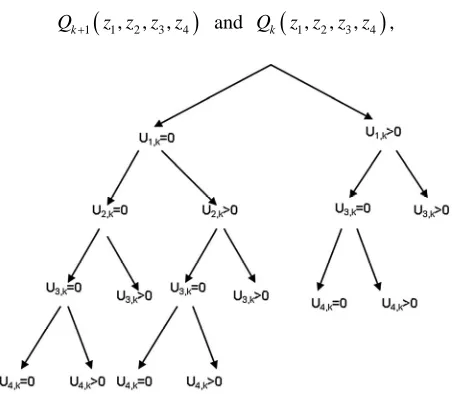
Taking the z-transform of the system Equations (1), and by considering the nine cases depicted in Figure 2, we derive, by means of some standard z-transform ma- nipulations, the following relationship between
1 1, 2, 3, 4
k
[image:3.595.311.537.509.706.2]Q z z z z and Qk
z z z z1, 2, 3, 4
,
1, 2, 3, 4
Q z z z z
0, , 0,
Q z z
4
, 0
k z
3 0
z
and then in Equation (3). Then: as illustrated in Equation (3) (below).
Next, we define the steady-state JPGF of the system
contents: Q z z
1, 2, 0, 0
A z z
1, 2
B 0, 0 (5) where:
1, 2, 3, 4
lim k kQ Q z z z z
z
Applying the above limit to Equation (3) yields (see
Equation (4) below):
Although it was not possible to determine all the seven boundary functions appearing in (4), as one of the 2
un-known boundary terms ( or 2 4 )
could not be determined, we were able to derive the relevant performance measures related to mean system contents at each node and mean delays. It should be noted that the strong coupling between node 4 and the remaining nodes made the direct application of standard pgf techniques to extract all the boundary terms, appear-ing in (4), an intricate task.
0, 0, 3, 4
Q z z
4. Determination of Relevant Boundary
Terms
In this section, we show how to progressively determine some unknown boundary terms in order to extract rele-vant performance measures for the queuing model under consideration.
4.1. Determination of Q (z1, z2, 0, 0), Q (0, z2, 0, 0)
and Q (0,0,0,0)
First, to determine Q z
1,z2, 0, 0
, let4 3
4 3
3 4
0 0
0, 0, 0, 0
0, 0, , 0 0, 0, 0,
z z
Q
Q z
Q z
z z
(6)
Next, to determine the constant , we set z1=z2=1 in Equation (5), which yields:
1,1, 0, 00, 0
Q B
z z z z z
(7)
The boundary constant Q (1,1,0,0) is readily obtained from the normalization condition Q (1,1,1,1) = 1. In fact by setting 1 2 3 4
in Equation (4), it is easy to derive the following expression for the PGF of the total system content:
1 , , 0, 0T T
T
T T
A z B z z Q z z Q z
z A z B z
(8)
1 1T
Q leads to
The normalization condition
1,1, 0, 0
1Q T. By substituting this result back into
Equation (7) and then into Equation (5), we immediately obtain the first unknown boundary function:
1, 2, 0, 0
1 T
1, 2
Q z z A z z (9)
2, 1 3, 1 4, 1
2 4
1 2 3 4 4 3 4 4
4 3
4
2 2 4 4 2
2 2
3
1 1
, , 0, 0, 0, 0 0, 0, 0, 0, 0, 0, 0 0, 0, , 0, 0, 0,
1
0, , 0, 0 0, 0, 0, 0 0, , 0, 0, 0, 0, 0, , 0
k k k k
u u u u
k k k k k
k k k k k
z z z
A z z B z z Q Q z Q Q z z Q z
z z
z
Q z Q Q z z Q z Q z
z z
1, 1
1 1, 2, 3, 4 1
k
Q z z z z E z
4
4 3 4 2 4 4
2 3
1 2 3 4 2 3 4 1 2 4 2 4
1
3 3
1 2 2 1 2 4 2 4 1
1 1 4
, 0 0, 0, 0, 0
0, 0, 0, , 0, , 0, 0, 0, 0,
1
, , , 0, , , , , 0, 0, , 0,
, , 0, 0 0, , 0, 0 , , 0, 0, , 0,
k
k k k k
k k k k
k k k k k
Q
z
Q z z Q z z Q z z Q z
z z
Q z z z z Q z z z Q z z z Q z z
z
z z
Q z z Q z Q z z z Q z z Q z
z z z
,z2, 0, 0
Qk
0,z2, 0, 0
(3)
2, 3, z
4 1 4 2 3 2 3 4 2 3 3 4 1 2 4 2
3 4 1 4 2 3 2 4 2 3 4 1 2
1 3 4 2 4 4 1 4 2 4 3 4
3 4 1 4 2 3 2 1 3 4 2 4
4
2 3 4
0, , , , , 0,
0, , 0, 1 , , 0, 0
0, 0, 0, 0, 0, ,
1 0, , 0, 0 1 0, 0, 0, 0
z z z z z Q z z z z z z z Q z z z
z z z z z z Q z z z z z Q z z
z z z z z Q z z z z z Q z z
z z z z z z Q z z z z z z Q
Q A z
z z z z
z
1, 2 3, z z B z
1 A z z1, 2 B z z3, 4
The other two related boundary terms are readily de- rived from Equation (9):
0, 2, 0, 0
1Q z
T
A 0,z2
1 T
AT 0
0, 0, 0, 0
0 T 1(10)
0, 0, 0, 0
Q (11)
and therefore for the system to be stable, we require that or equivalently,
Q
.4.2. Relationship between Q (z1, z2, 0, z4) and
Q (0, z2, 0, z4)
In this subsection, we determine 1 2 4
up to the boundary term, , 0,
Q z z z
0, 2, 0, 4
Q z z
,
0,A z z B
. For this purpose, let and in Equation (3). Then:
k z30
, , 0,
Q z z1 2 z4 1 2
z4
z z2, 4
(12) where:
3
2 4
4 4
3 4 4
2
3 0 2
2 3 4 3 4
4
2 3
2 4 4
2
( , )
1
0, 0, 0, 0 0, 0, 0, 0, 0, 0
0, 0, ,
0, , 0, 0
0, , , 0, 0, ,
1
0, , 0, 0, 0, 0, 0,
0, 0, 0, 0
z
z z
Q Q z
z
Q z z z
Q z
z z
Q z z z Q z
z
z z z
Q z z Q z Q
z
Q
3 0 3 3 0
2 , 0
0, 0, 0, 0
, 0, 0
z z
Q
Q
z
z
is independent of z1. Substituting z1 = 0 in Equation (12), we get:
2 4
2 4
0, , 0, 0,
Q z z
2, 4
0,
z z
A z B z
and therefore:
Q 0,z2, 0,z4
1 2
1 2 4
2
, , , 0,
0,
A z z Q z z z
A z
(13)
Thus
4.3. Determination of Q (0, 0, z, z) and Q (0, z, 0, z)
1, 2, 0, 4 Q z z z
is determined up to the bound- ary term Q 0,z2, 0,z4
.
To determine the boundary term Q 0, 0, ,z z
, we pro- ceed as follows:
First by setting z1 = z2 = x and z3 = z4 = z in Equation (4), we obtain (see Equation (14) below):
From (9), we note that Q x x, , 0, 0 1 T AT x
.Also sinceQ x x z z
, , ,
is analytic inside the polydisk (
x 1,z 1
), then the numerator must be zero when- ever the denominator is zero. It follows that:
0, 0, ,
0
1 T 1 T z z T
z
Q z z
zA Y Y z A
z
z Y
(15)
where Yz is the unique solution for x in the unit disk
z 1
of the equation xAT
x BT z 0.
Next, we determine Q 0, , 0,z z
by proceedings as follows:
First by setting z1 = z3 = x and z2 = z4 = z in Equation (4), we obtain (see Equation (16) below):
From (9), we note that Q x x, , 0, 0 1 T AT x
. Also from (13):
,
, , 0, 0, , 0,
0,
A x z
Q x z z Q z z
A z
(17)
Substituting for Q x x, , 0, 0
and Q x z
, , 0,z
in (16) and since Q x
, , ,z x z
is analytic inside the polydisk
x 1,z 1
, then from Rouche’s theorem, we get:
0, , 0, 1 1 0, z
T
z R
Q z z z A z
z R
(18)
where Rz is the unique solution for x of the equation
, ,xA x z B x z in the unit circle x 1.
5. Joint and Marginal PGFs
Having determined some relevant boundary terms, we can now easily derive the marginal PGFs of the system contents at nodes 1, 2, and 3, as well as several other JPGFs. This is illustrated below.
5.1. Joint and Marginal PGFs of High-Priority (Class-1) System Contents
Let P13 z z1, 3 Q z1,1,z3,1
denote the JPGF of the
0, 0, , 1 , , 0, 0 1 0, 0, 0, 0, , ,
T T
x z Q z z z z Q x x z x z Q
Q x x z z z
z x A x B z
T T
A x B (14)
, , ,
, ,
, , 0,
1
, , 0, 0
, ,
x z Q x z z x z Q x z Q x z x z A x z B x z
z x A x z B x z
(16)
system contents of the high-priority queues at nodes 1 and 3. By setting z2 = z4 = 1 in Equation (4), we get (see Equation (19) below):
To determine the boundary terms P13
z1, 0
and
13 0, 0 P
, appearing in (19), we first set z2 = z4 = 1 in (13):
1
113 0, 0 0
P z P
A
13 1
1
, 0 A z (20)
Next, from (19), the normalization condition P13 (1, 1) = 1yields P13
1, 0 1 1 3. Therefore setting z11 in (20), we get:
13 1
13 1 1
0, 0 1
, 0 1
P z
3 1 3 1 10 P A A z
(21)The remaining boundary term P13 0,z3
is readily obtained by substituting (20) and (21) into (19) and by invoking the analytical property of P13 0,z3
inside the polydisk
z 1;z
1 . It follows from Rouche’s
theorem that:
3 1
3 33
3 1 0
z
z A
13 3
3 1 1 3 3
3 0,
1 1 z z
P z
z A X X
z z X (22)
where for a given z3
z3 1
, Xz3
is the unique solu- tion for z1 of the equation z1 A z B1 1
3
z3 in the unit circle z3 1.Substituting (21) and (22) back into (19), we obtain after few algebraic manipulations:
3 3 3 3 3 1 3 13 1 z z z z z X
z A X
z
13 1 31 3 1 1 3 3
3 1 1
1 1 1 3 ,
1
P z z
A z B z
z X A z z
z A z B
(23)
From the above, we can obtain expressions for the following:
Marginal PGF of the number of class-1 customers in queue 1:
1 1 11 1 1 1
z A z
z A z
1 1 13 1,1 1 1
P z P z (24)
Marginal PGF of the number of class-1 customers in queue 3:
3 3
3
3 3 13 3 1 3 3 3
3 3 1
3
3 3 3
1, 1 1 1 1 z z z
P z P z
B z
z X z A X
z
z X B z
(25)
PGF of the total number of class-1 customers in the system:
2
1 3 1 3
13, 13
1 3
1 1
,
T
z A z B z
P z P z z
z A z B z
(26)It should be noted that since the high-priority traffic (traversing nodes 1 and 3) is not influenced by the low-priority traffic (traversing nodes 2 and 4), then the above results for the JPGF P1,3 z z1, 3
could have been derived by analyzing the performance of the two tandem queues 1 and 3, independently from the rest of the system. We carried this analysis and confirmed that the resulting JPGF of the system contents matches the one derived in Equation (23).5.2. Joint PGFs of the System Contents in PQS1
Let P12 z z1, 2 Q z z1, 2,1,1
denote the JPGF of the system contents of the first priority queuing system(PQS 1). Then from Equation (4):
12 1 2
1 2 12 2 1 2 12 1 2
2 1 1 2 ,
0, 1 0, 0
,
,
P z z
z z P z z z P
A z z
z z A z z
(27)The boundary constant 12
is readily obtained from the normalization condition 12 , yielding0, 0
P
1,1 1P
0, 0 1P12 1 2. The boundary term P12
0,z2
is readily obtained from (27) by applying Rouche’s theo-rem:
2
2 2
12 2 1 2
2 1
0, 1 z
z
z
P z W
z W
(28)
where for a given z2
z2 1
, Wz2
1 1, 2
z A z z
is the unique solu-tion for z1 of the equation in the unit cir-cle z2 1.
12 0, 2
P z and
Next, by substituting for P12 0, 0 back into (27), we get:
2
2 12 1 2
1 2
1 2 1 2
2 1 1 2
, 1 1 , , z z
P z z
z W
z A z z
z W z A z z
(29)
3 3 13 1 1 3 13 3 3 1 3 133 1 1 1 3 3
1 , 0 0, 1 0, 0
z z P z z z P z z z z P
z
z z A z B z
13 1, 3 1 1 3 3
From the above, we can obtain expressions for the
following:
Marginal PGF of the number of class-1 customers in queue 1:
1
1 1 1 1 11
z A z
z A z
1 1 12 1,1 1 1
P z P z (30)
Marginal PGF of the number of class-2 customers in queue 2:
22
2 2 2
1 1 z z W A z
2 2 1,2 22 1 2 2 2
1,
1 1
P z P z
z A z z W (31)
PGF of the total number of class-1 customers in PQS1
1 2
12,T 12 ,
P z P z z
z A
1 1 T
T
z A z
z
, 1,1, ,
(32)
We also observe that the JPGF of the system contents of PQS 1 could have also been be derived by considering PQS 1 as an isolated priority queuing system. Such an analysis of a single stage PQS has been presented in [5] and our expressions (31-32) match those derived therein.
5.3. PGFs of Total Number of Customers in PQS2
Let P34,T
z P34
z z Q z z denote the JPGF of the total number if customers in the second priority queuing system (PQS 2). Then from (4):
34, 11,1, 0, 0 0, 0, , 1
1
T T
T
P z
z B z
zQ Q z z z
z B z
0, 0, 0, 0 Q
(33)
Using (9), (11) and (15), we can determine the un-known boundary terms appearing in the above equation, yielding:
34, 1 1 1 TT T z
z T
P z
z B z z Y
z Y B z
1 T z
z A Y
(34)
where, as defined earlier, for a given z z
1
0T x BT z
, Yz is the
unique solution for x of the equation in the unit circle
x A x 1
, 1, ,1,
.
5.4. PGF of the Total Number of Class-2 Customers in the System
Let P24,T
z P24
z z Q z z denote the PGF of the total number of class-2 customers in the system. Then from Equation (4):24,
2
2 4
2 4
1 1, , 0,
1
1
T
T
P z
A z Q z z
z A z B z
z A z B z
1, , 0,
Q z z
(35)
The unknown boundary term can be de-termined from (13) and (18), which yields:
2
2 4
24,
2 4
1 1 1
1
T z
T
z A z B z R
P z
z
A z B z z R
(36)
where Rz is the unique solution for x of the equation
, ,xA x z B x z inside the unit circle x1.
5.5. PGF of the Total System Contents
, , ,
T
P
Let z Q z z z z
denote the PGF of the total system contents. Then using (4) and (9) we get:
2
1 1 T T
T T
T T
A z B z
P z z
z A z B z
(37)
6. Calculation of the Moments
To compute the various moments of system contents, we introduce and recall the following notations:
1 2 3 4 2 1 2 1 2 3 4 1 ,, 1, 2 1, 2
,
, 3, 4 3, 4
i j
i j
z z
ij
z z
A z z
i j z z
B z z
i j z z
1 1 1 2
2 1 3 4
d 1 d d 1 d T
T T z
T
T T z
A z A z B z B z
21 11 22 12
2 2
1 33 44 34
2 d 1 2 d d 1 2 d T T z T T z A z A z B z B z , , , (38)
Next, we observe that the functions Xz3 Wz2 Y Rz z
1 i z
, appearing in the various pgfs of the system contents, can only be explicitly defined under simple arrival processes. Fortunately, the derivation of the first and higher mo-ments of the system contents involves evaluating these functions and their first and higher order derivatives at
. These can be readily computed in closed-form. From the corresponding pgfs (24 - 26, 30 - 32, and 34, 36 - 37), the mean system content of class-j customers (j
= 1, 2) and the mean total system contents are readily obtained:
11
1 1 2 1 1 1 1
N P
(39)
Mean system content of class-1 customers at node 3:
11
11
33
3 12 1 2 1
N 3 3
1 1 3
2 1
(40)
Total mean system contents of class-1 customers:
11
13,T 13,T 1 2 1 3
N P 1 3 33
1 3 2 2 1
(41)
Mean system content of class-2 customers at node 2:
12 22
2 2 2
2 1
2 1 2 1
N P 2 11
1T 1T 1 1
(42)
Total mean system contents of class-2 customers:
24,
24, 2
3 3 11 33 1 3 1 1 1 2 2 1 2 1 2 1 T T T T T N A B P 2 2
2T 1T
(43)
Mean system content of class-2 customers at node 4:
The mean number of class-2 customers at node 4 can be derived by subtracting the mean system content of class-2 customers at node 2 from the total mean system contents of class-2 customer. Hence, using (42) and (43), we get:
4 24, 2
2 2
2
1
3 3 11 33
1 3 1
1 1 2 1
2 1
2 1
2 1 2 1
T
T T T
T
T
N N N
A B 12 22
1 2 1 2 1 T (44)
Total mean system contents at PQS1:
12,T 12,T 1 1T
N P
1 1 2 1 T T A
(45)
Total mean system content at PQS2:
34, 34, 2 1 11 1 2
2 1
T T
T T T
T
N P
A B
1 1 2 1 T T T T A (46)
Total mean system content
It can be easily verified that Equations (39-47) satisfy the expected results:
12, 1 2 34, 3 4 13, 1 3
1 2 3 4
T
T
T
T
N N N
N N N
N N N
N N N N N
(48)
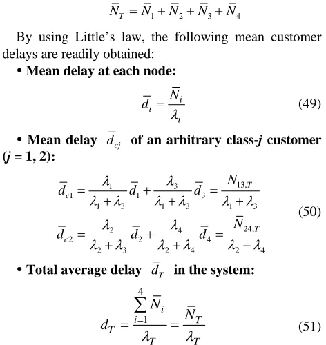
By using Little’s law, the following mean customer delays are readily obtained:
Mean delay at each node: i i
i
N
d (49)
Mean delay dcj of an arbitrary class-j customer
(j = 1, 2):
13, 3
1
1 1 3
1 3 1 3 1 3
24,
2 4
2 2 4
2 3 2 4 2 4
T c
T c
N
d d d
N
d d d
1 21 1 2 T T
T
1
1
2 1
T T
T T T T
A B
N P
(47)
(50)
Total average delay dT in the system: 4 1 i i T T T T N N d
(51)7. Numerical Examples and Discussions
In this section, we illustrate our approach through some numerical examples. In particular, we will further probe into the influence of HOL priority on the performance of low-priority traffic stream. For this purpose, we consider two-dimensional Binomial exogenous arrival processes with JPGFs:
1 2
1, 2 1 1 1 1 2
N
A z z z z
N N
3
3
3, 4 1 1 3 1 4
N
B z z z z
N N
Further, we define i i T (i = 1, 2, 3) as the
fraction of arrivals to node i among the total arrivals. For the numerical calculations, we have set N = 16 and
1 2 3
In Figure 3, the mean customer delay at each node as well as the total average delay, are plotted as a function of the total arrival rate T
, , 0.45, 0.25, 0.20
.
. The mean delay i at each
node and the total average delay
d
T were computed by
substituting for
d
i as given in Equations (39), (40),
(42), and (44) into (49) and (51), respectively.
[image:8.595.306.542.166.416.2]N
Figure 3. Mean delays versus total arrival rate T.
Figure 4. Mean delay of a class-j customer (j = 1, 2).
customer (j = 1, 2) and the total average delay as a func-tion of the total arrival rate T. In this case, the mean
delay T for each class j customer was computed by
substituting for N13,T and N24,T, as given in Equations
(41) and (43), into (50).
As may be seen from the above figures, the HOL pri-ority scheduling has a significant influence on the mean delay of the low-priority (class-2) customers. This star-vation effect is even more significant at node 4. To this regards, recall that class-2 customers arriving at the ac-cess node (2) are subjected to two consecutive HOL in-terruption processes due to the potential presence of higher priority customers at nodes 1 and 3. The above results not only echo but also amplify previous concerns related to the unfairness of the static HOL priority scheduling mechanism for low-priority traffic. Therefore HOL scheduling should be used with caution.
Our research also suggests that more research is needed to come-up with efficient priority mechanisms that exhibit better fairness and that can be easily imple-mented in real-time. Earlier contributions in this regards focused on a class of dynamic priority schemes that are
based on the queue-length-threshold scheduling disci-pline. Under this scheme, the priority scheduling can dynamically change, based on the queue lengths (see for example [11-15]) [16]. Some More recent contributions include the work of Maertens et al. [17-19] on priority jumping mechanisms and the contribution of De Vuyst et al. [20,21] on reservation-based priority disciplines.
8. Conclusions and Future Research
In this paper, we presented an exact analysis of a two HOL priority queuing systems in a tandem configuration. For each PQS, our model allows for possible correlation between the numbers of arrivals of the two classes of customers during a slot. We showed how a generating function approach can be used to derive closed-form ex-pressions for several performance measures. Finally we have demonstrated, via numerical examples, the negative impact the HOL priority scheduling on performance of the low-priority traffic.
This work can be further explored in many directions. For instance, it would be interesting to derive expressions for the pgf of customer delay and characterize the end- to-end delay of a tagged customer. The characterization of the asymptotic behavior of the tail distributions of the various system contents is still an open research issue.
Finally, our analysis can also be extended to handle the case where customers leaving the first PQS stage are allowed to leave the system with a pre-assigned probabil-ity. These are left for future research.
REFERENCES
[1] A. Khamisy and M. Sidi, “Discrete-Time Priority Queues with Two-State Markov Modulated Arrivals,” Stochastic Models, Vol. 8, No. 2, 1992, pp. 337-357.
doi:10.1080/15326349208807228
[2] M. Sidiand and A. Segall, “Structured Priority Queuing Systems with Applications to Packet-Radio Networks,”
Performance Evaluation, Vol. 3, No. 4, 1983, pp. 265- 275. doi:10.1016/0166-5316(83)90036-6
[3] T. Takine, B. Sengupta and T. Hasegawa, “An Analysis of a Discrete-Time Queue for Broadband ISDNwith Pri-orities among Traffic Classes,” IEEE Transactions on Communications, Vol. 42, No. 2-4, 1994, pp. 1837-1845.
doi:10.1109/TCOMM.1994.582893
[4] T. Takine, “A NonpreemptivePriority MAP/G/1 Queue with Two Classes of Customers,” Journal of Operations Research Society of Japan, Vol. 39, No. 2, 1996, pp. 266- 290.
[5] J. Walraevens, B. Steyaertand H. Bruneel,” Performance Analysis of a Single-Server ATM Queue with a Priority Scheduling,” Computers and Operations Research, Vol. 30, No. 12, 2003, pp. 1807-1829.
doi:10.1016/S0305-0548(02)00108-9
[image:9.595.59.290.269.439.2]Analysis of a Discrete-Time Priority Queue,” Proceed-ings of the 12th International Conference on Analytical and Stochastic Modelling Techniques and Applications
(ASMTA 2005), Riga, June 2005, pp. 17-24.
[7] K. Laevens and H. Bruneel, “Discrete-Time Multiserver Queues with Priorities,” Performance Evaluation, Vol. 33, No. 4, 1998, pp. 249-275.
doi:10.1016/S0166-5316(98)00024-8
[8] J. Walraevens, D. Fiems, S. Wittevrongel and H. Bruneel, “Calculation of Output Characteristics of a Priority Queue through a Busy Period Analysis,” European Journal of Operational Research, Vol. 198, No. 3, 2009, pp. 891-898.
doi:10.1016/j.ejor.2008.11.018
[9] F. Kamoun, “Performance Analysis of a Non-Preemptive Priority Queuing System Subjected to a Correlated Mark-ovian Interruption Process,” Computers and Operations Research, Vol. 35, No. 12, 2008, pp. 3969-3988.
doi:10.1016/j.cor.2007.06.001
[10] J. Walraevens, D. Fiems and H. Bruneel, “The Discrete- Time Preemptive Repeat Identical Priority Queue,” Queu- ing Systems, Vol. 53, No. 4, 2006, pp. 231-243.
doi:10.1007/s11134-006-7770-x
[11] R. Chipalkatti, J. F. Kurose and D. Towsley, “Scheduling Policies for Real-Time and Nonreal-Time Traffic Packet Switching Node,” Proceedings of the IEEE INFOCOM ’89, Ottawa, April 1998, pp. 774-783.
[12] B. I. Choi and Y. Lee, “Performance Analysis of a Dy- namic Priority Queue for Traffic Control of Bursty Traf- fics in ATM Networks,” IEEE Proceedings of Commu- nications, Vol. 148, No. 3, 2001, pp. 181-187.
doi:10.1049/ip-com:20010115
[13] D. I. Choi, B. D. Choi and D. Sung, “Performance Analy- sis of Priority Leaky Bucket Scheme with Queue- Length-Threshold Scheduling Policy,” IEEE Proceedings of Communications, Vol. 145, No. 6, 1998, pp. 395-401.
doi:10.1049/ip-com:19982287
[14] C. Knessl, D. I. Choi and C. Trier, “A Dynamic Priority Queue Model for Simultaneous Service of Voice and
Data Traffic,” SIAM Journal on Applied Mathematics, Vol. 63, No. 2, 2002, pp. 398-422.
doi:10.1137/S0036139901390842
[15] J. T. Lee and Y. H. Kim, “Performance Analysis of a Hybrid Priority Control Scheme for Input and Output Queuing ATM Switches,” Proceedings of INFOCOM ’98, San Francisco, 29 March-2 April 1998, pp.1470-1477.
doi:10.1109/INFCOM.1998.662965
[16] T. Maertens, J. Walraevens and H. Bruneel, “Performance Analysis of a Single-Server Queue with HOL-PJ Priority Scheduling Discipline,” Proceedings of the Second In-ternational Working Conference on Performance Model-ling and Evaluation of Heterogeneous Networks (HET- NETs ’04), Ilkley, 26-28 July 2004, pp. 1-10.
[17] T. Maertens, J. Walraevens and H. Bruneel, “On Priority Queues with Priority Jumps,” Performance Evaluation, Vol. 63, No. 12, 2006, pp. 1235-1252.
doi:10.1016/j.peva.2005.12.003
[18] T. Maertens, J. Walraevens and H. Bruneel, “A Modified HOL Priority Scheduling Discipline: Performance Analy- sis,” European Journal of Operational Research, Vol. 180, No. 3, 2007, pp. 1168-1185.
doi:10.1016/j.ejor.2006.05.004
[19] T. Maertens, J. Walraevens, M. Moeneclaey and H. Bruneel,” Performance Analysis of a Discrete-Time Queu- ing System with Priority Jumps,” International Journal of Electronics and Communications, Vol. 63, No. 10, 2009, pp. 853-858. doi:10.1016/j.aeue.2008.07.004
[20] S. De Vuyst, S. Wittevrongel, D. Fiems and H. Bruneel, “Controlling the Delay Trade-off Between Packet Flows UsingMultiple Reserved Places,” Performance Evalua-tion, Vol. 65, No. 6-7, 2008, pp. 484-511.
doi:10.1016/j.peva.2007.12.008
[21] S. De Vuyst, D. Wittevrongel and H. Bruneel, “Place Reservation: Delay Analysis of a Novel Scheduling Me- chanism,” Computers and Operations Research, Vol. 35, No. 8, 2008, pp. 2447-2462.