An EOQ Model for Deteriorating Items with Linear Demand, Variable Deterioration and Partial Backlogging

An EOQ Model for Deteriorating Items with Linear

Demand, Variable Deterioration and Partial Backlogging

Trailokyanath Singh1, Hadibandhu Pattnayak2

1_{Department of Mathematics, C. V. Raman College of Engineering, Bhubaneswar, India;} 2_{Department of Mathematics, Sailabala} Women’s College, Cuttack, India.

Email: [email protected], [email protected]

Received January 26th_{, 2013; revised March 2}nd_{, 2013; accepted March 12}th_{, 2013}

Copyright © 2013 Trailokyanath Singh, Hadibandhu Pattnayak. This is an open access article distributed under the Creative Com-mons Attribution License, which permits unrestricted use, distribution, and reproduction in any medium, provided the original work is properly cited.

ABSTRACT

In this paper, an economic order quantity (EOQ) model is developed for deteriorating items with linear demand pattern and variable deterioration rate. Shortages are allowed and partially backlogged. The backlogging rate is variable and dependent on the waiting time for the next replenishment. The objective of the model is to develop an optimal policy that minimizes the average total cost. The numerical example is used to illustrate the developed model. Sensitivity analysis of the optimal solution with respect to various parameters is carried out.

Keywords: Deteriorating Items; Economic Order Quantity (EOQ); Linear Demand; Partial Backlogging; Variable

Deterioration Rate

1. Introduction

Recently, deteriorating items in inventory system have become an interesting feature for its practical importance. Generally, deterioration is defined as damage, decay or spoilage. Food items, photographic films, drugs, chemi-cals, pharmaceutichemi-cals, electronic components and radio-active substances are some examples of items in which sufficient deterioration may occur during the normal storage period of units and consequently the loss must be taken into account while analyzing the inventory system. Spoilage in food grain storage, decay in radioactive ele-ments, pilferages from on-hand inventory is continuous in time. Therefore, the effect of deterioration of physical goods cannot be disregarded in many inventory systems. Ghare and Schrader [1] first derived a revised economic order quantity by assuming exponential decay. Covert and Philip [2] extended Ghare and Schrader’s constant deterioration rate to a two-parameter Weibull distribution. Later, Shah and Jaiswal [3] and Aggarwal [4] presented and re-established an order level inventory model with a constant rate of deterioration respectively. Dave and Patel [5] considered an inventory model for deteriorating items with time-proportional demand when shortages were not allowed. Later, Sachan [6] extended the model to all for shortages. Hollier and Mak [7], Hariga and

Benkherouf [8], Wee [9,10] developed their models tak-ing the exponential demand. Earlier, Goyal and Giri [11], wrote an excellent survey on the recent trends in model-ing of deterioratmodel-ing inventory. For the items like fruits and vegetables, whose deterioration rate increases with time. Ghare and Schrader [1] were the first to use the concept of deterioration followed by Covert and Philip [2] who formulated a model with variable rate of deteriora- tion with two-parameter Weibull distributions, which was further extended by Philip [12] considering a vari- able deterioration rate of three-parameter Weibull distri- butions. In some inventory systems, the longer the wait- ing time is, the smaller the backlogging rate would be and vice versa. Therefore, during the shortage period, the backlogging rate is variable and dependent on the wait- ing time for the next replenishment. Chang and Dye [13] developed an EOQ model allowing shortage. Recently, Ouyang, Wu and Cheng [14] established an EOQ inven- tory model for deteriorating items in which demand function is exponential declining and partially backlog- ging.

time for the next replenishment. Ever till now, most of the researchers have been either completely ignoring the deterioration factor or are considering a constant rate of deterioration, which is not possible practical. Since the effect of deterioration cannot be ignored, we have taken a variable deterioration. The objective of the model is to determine the optimal order quantity and the length of the ordering cycle in order to minimize the total relevant cost. A numerical example is cited to illustrate the model and a sensitivity analysis of the optimal solution is car-ried out.

2. Assumptions

The following assumptions are made in developing the model.

1) The inventory system involves only one item and the planning horizon is infinite.

2) Replenishment occurs instantaneously at an infinite rate.

3) The deteriorating rate 

 

t t, 01, is a

variable deterioration and there is no replacement or repair of deteriorated units during the period under consideration.

4) The demand rate, ,

, where

 

_{ }

 

0

, 0

, 0

a bt I t D t

D I t

 



  _



0, 0

a b and a is initial demand.

5) During the shortage period, the backlogging rate is variable and is dependent on the length of the waiting time for the next replenishment. The longer the wait- ing time is, the smaller the backlogging rate would be. Hence, the proportion of customers who would like to accept backlogging at time t is decreasing with the

waiting time



Tt



waiting for the next replenish-

ment. To take care of this situation we have defined

the backlogging rate to be



1



1 Tt when in ven-

tory is negative. The backlogging parameter  is a positive constant, t1 t T.

3. Notations

The following notations have been used in developing the model.

1) C1: holding cost, $/per unit/per unit time.

2) C2: cost of the inventory item, $/per unit.

3) C3: ordering cost of inventory, $/per order.

4) C4: shortage cost, $/per unit/per unit time.

5) C₅: opportunity cost due to lost sales, $/per unit.

6) t1: time at which shortages start.

7) T : length of each ordering cycle.

8) W : the maximum inventory level for each ordering

cycle.

9) S: the maximum amount of demand backlogged

for each ordering cycle.

10) Q: the economic order quantity for each ordering

cycle.

11) I t

 

: the inventory level at time t.

12) t1: the optimal solution of t1.

13) T: the optimal solution of T.

14) Q: the optimal economic order quantity.

15) W: the optimal maximum inventory level.

16) TC: the minimum average total cost per unit time.

4. Mathematical Formulation

We consider the deteriorating inventory model with lin- ear demand. Replenishment occurs at time t0 when

the inventory level attains its maximum, W . From

0

t to ₁, the inventory level reduces due to demand

and deterioration. At time 1 , the inventory level

achieves zero, then shortage is allowed to occur during the time interval

t

t

 

t T1, and all of the demand during

shortage period

 

t T1, is partially backlogged.

As the inventory level reduces due to demand rate as well as deterioration during the inventory interval

 

t T1, ,

the differential equation representing the inventory status is governed by

 

_{   }

_{ }

1

d

, 0 d

I t

t I t D t t t

t      , (1)

where 

 

t t and D t

 

 a bt.

The solution of Equation (1) using the condition

 

1 0 I t  is

 

2

2

3 2 4

1 1 1 2

1

3 2 4

2

1

e

6 2 8

e , 0

6 2 8

t

t

t t t

I t a t b

t t t

a t b t t

 

 

 





    

      

    

 

    

        

    

 

.(2)

(neglecting the higher power of  as 01). Maximum inventory level for each cycle is obtained by putting the boundary condition I

 

0 W in Equa-

tion (2). Therefore,

 

13 12 1 1

0

6 2 8

t t t

I W a t_  _b_ 

  

4

 



 . (3)

During the shortage interval

 

t T1, , the demand at

time is partially backlogged at the fraction t



1



1 Tt . Therefore, the differential equation gov-

erning the amount of demand backlogged is

 



0



1

d

,

d 1

I t D

t t T

t    Tt   . (4)

 









0 0 1 1 ln 1

ln 1 ,

D

I t T t

D

T t t t T

     _   _  _   _  

. (5)

Maximum amount of demand backlogged per cycle is obtained by putting tT in Equation (5). Therefore,

 

0





1

ln 1

D

S I T  T t



   _   _ . (6)

Hence, the economic order quantity per cycle is





3 2 1 1 1 0 1

6 2 8

ln 1

t t t

Q W S a t b

D T t    4 1                 _   _  

. (7)

The inventory holding cost per cycle is

 

1 2 1 2 1 1 0

3 2 4

1 1 1 2

1 1

0

3 2 4

2 1

0

2 4 3 5

1 1 1 1

1

d

e d

6 2 8

e d

6 2 8

2 12 3 15

t

t t

t t

HC C I t t

t t t

C a t b t

t t t

C a t b t

t t t t

C a b

                 _{ }                  _{ }  _ _  _                           







   

. (8)

(neglecting the higher power of  as 01). The deterioration cost per cycle is

 





1 1 2 0 3 4 1 1 2 2 0 d d 6 8 t t

DC C W D t t

at bt

C W a bt t C

   _  _                      





. (9)

The shortage cost per cycle is

 

























1 1 4 4 0 1 1

4 0 2 1

d

ln 1 ln 1 d

1 ln 1 T t T t

SC C I t t

C D

T t T t t

T t

C D T t

                   _      _     _    _  





. (10) The opportunity cost due to lost sales per cycle is













1

5 0

5 0 1 1

1 1 d 1 1 ln 1 T t

OC C D t

T t

C D T t T t

        _  _             



Therefore, the average total cost per unit time per cy- cle = (holding cost + deterioration cost + ordering cost + shortage cost + opportunity cost due to lost sales)/length of the ordering cycle, i.e.,















_

_

1

2 4 3 5

1 1 1 1 1

3 4

1 1

2 3

0 4 5 1

0 4 5

1 2

,

2 12 3 15

1

6 8

ln 1

TC TC t T

C t t t t

a b

T

at bt

C C

T

D C C T t

T

D C C

T t T                                                    _   _

. (12)

Our aim is to determine the optimal values of 1 and

in order to minimize the average total cost per unit time, .

t T

TC

Using calculus, we now minimize . The optimum values of 1 and T for the minimum average cost

are the solutions of the equations

TC t TC

 

1 0 TC t  

 and

 

0 TC T  

 , (13)

provided that they satisfy the sufficient conditions

 

2 2 1 0 TC t    ,

 

2 2 0 TC T  

 and

 

 

 

2

2 2 2

2 2

1 1

0

TC TC TC

t T t T       _ _      _{ } .

Equation (13) can be written as

 



















2

1 1 1 2

1 1

0 4 5 1

1

1

3 2

0 1

TC t a bt t C t

C

t T

D C C T t

T T t

    1              _{   }      

. (14)

and

 











 

0 4 5 1

1

1 ₀

1

D C C T t

TC

TC

T T T t

 

   



   

 _   _ . (15)

  

. (11)

Now, t1  _and

T are obtained from the Equations

(13) and (14) respectively. Next, by using t1  _and

T,

we can obtained the optimal economic order quantity, the optimal maximum inventory level and the minimum av-erage total cost per unit time from Equations (7), (3) and (12) respectively.

5. Numerical Example

trate the above theory.

Example 1: Let us take the parameter values of the in- ventory system as follows:

12

a , b2, C10.5, C₂1.5, C33, C42.5,

, ,

5 2

C  D₀8 0.01, and  2.

Solving Equations (14) and (15), we have the optimal shortage period 1 unit time and the optimal

length of ordering cycle unit time. Thereafter, we get the optimal order quantity

units, the optimal maximum inventory level units and the minimum average total cost per unit time .

0.84669

t 

T

168

TC

0.992958

_

5.8845 5.7381

Q

W4.71

6. Sensitivity Analysis

We study now study the effects of changes in the values of the system parameters , , ₁, ₂, ₃, ₄,

5, 0,

a b C C C C

C D  and  on the optimal total cost and num-

ber of reorder. The sensitivity analysis is performed by changing each of parameters by +50%, +10%, −10% and

−50% taking one parameter at a time and keeping the remaining parameters unchanged.

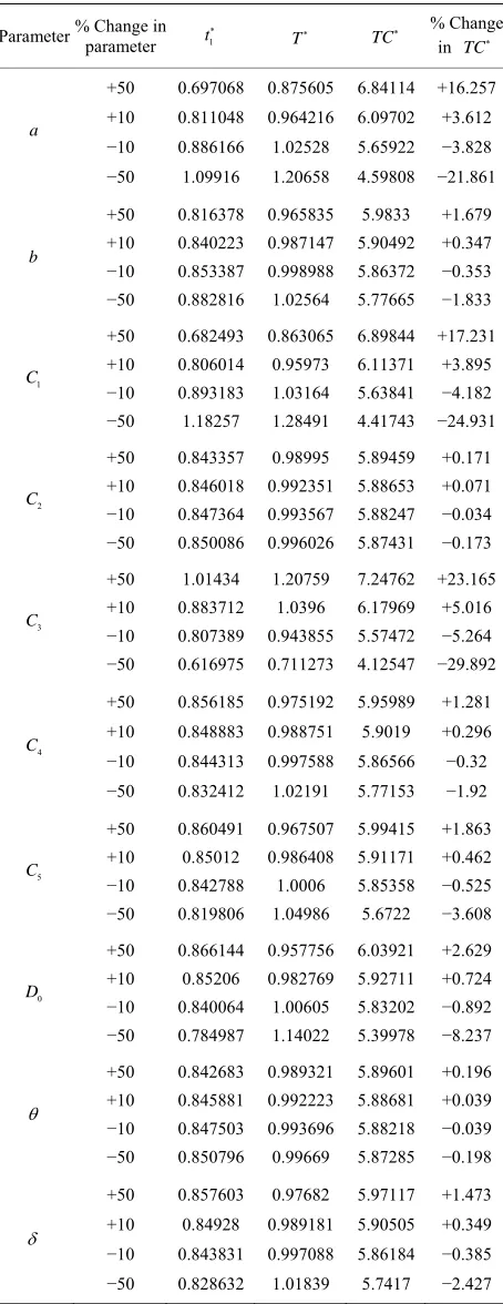
The analysis is based on the Example 1 and the results are shown in Table 1. The following points are observed.

1) t1  _&

T decrease while TC increases with the

increase in value of the parameter a. Both t1 & T are highly sensitivity to change in a and TC

is moderately sensitive to change in a.

2) t1  _&

T decrease while TC increases with the

increase in value of the parameter b. Both t1 &

T are moderately sensitive to change in b and TC is low sensitive to change in b.

3) t1 & T decrease while TC increases with the

increase in value of the parameter C₁. Here t1  _&

T and TC are highly sensitive to change in C1.

4) t1 & T decrease while TC increases with the

increase in value of the parameter C₂. Here t₁, T

and TC are low sensitive to change in C2.

5) t1 , T & TC increase with the increase in value

of the parameter C3. Here t1, T and TC are

highly sensitive to change in C₃.

6) t1  _&

TC increase while T decreases with the

increase in value of the parameter C4. Here t1 & T and TC are moderately sensitive to change in

4 C .

7) t1 & TC increase while T decreases with the

increase in value of the parameter C₅. Here t₁, T

and TC are moderately sensitive to change in C5.

8) t1 & TC

 _{increase while}

T decreases with the

increase in value of the parameter D0. Here t1, T

and TC are moderately sensitive to change in D0.

9) t1  _&

T decrease while TC increases with the

increase in value of the parameter . Here t1, T

[image:4.595.310.537.100.688.2]

and TC are low sensitive to change in .

Table 1. Sensitivity analysis.

Parameter% Change in _parameter t1



T TC % Change _{in TC}

a

+50 +10 −10 −50

0.697068 0.811048 0.886166 1.09916

0.875605 0.964216 1.02528 1.20658

6.84114 6.09702 5.65922 4.59808

+16.257 +3.612 −3.828 −21.861

b

+50 +10 −10 −50

0.816378 0.840223 0.853387 0.882816

0.965835 0.987147 0.998988 1.02564

5.9833 5.90492 5.86372 5.77665

+1.679 +0.347 −0.353 −1.833

1

C

+50 +10 −10 −50

0.682493 0.806014 0.893183 1.18257

0.863065 0.95973 1.03164 1.28491

6.89844 6.11371 5.63841 4.41743

+17.231 +3.895 −4.182 −24.931

2

C

+50 +10 −10 −50

0.843357 0.846018 0.847364 0.850086

0.98995 0.992351 0.993567 0.996026

5.89459 5.88653 5.88247 5.87431

+0.171 +0.071 −0.034 −0.173

3

C

+50 +10 −10 −50

1.01434 0.883712 0.807389 0.616975

1.20759 1.0396 0.943855 0.711273

7.24762 6.17969 5.57472 4.12547

+23.165 +5.016 −5.264 −29.892

4

C

+50 +10 −10 −50

0.856185 0.848883 0.844313 0.832412

0.975192 0.988751 0.997588 1.02191

5.95989 5.9019 5.86566 5.77153

+1.281 +0.296 −0.32 −1.92

5

C

+50 +10 −10 −50

0.860491 0.85012 0.842788 0.819806

0.967507 0.986408 1.0006 1.04986

5.99415 5.91171 5.85358 5.6722

+1.863 +0.462 −0.525 −3.608

0

D

+50 +10 −10 −50

0.866144 0.85206 0.840064 0.784987

0.957756 0.982769 1.00605 1.14022

6.03921 5.92711 5.83202 5.39978

+2.629 +0.724 −0.892 −8.237



+50 +10 −10 −50

0.842683 0.845881 0.847503 0.850796

0.989321 0.992223 0.993696 0.99669

5.89601 5.88681 5.88218 5.87285

+0.196 +0.039 −0.039 −0.198



+50 +10 −10 −50

0.857603 0.84928 0.843831 0.828632

0.97682 0.989181 0.997088 1.01839

5.97117 5.90505 5.86184 5.7417

+1.473 +0.349 −0.385 −2.427

10) t₁ & TC increase while T decreases with the

increase in value of the parameter  . Here t₁, T

7. Conclusions

The economic order quantity (EOQ) model considered above is suited for items having variable deterioration rate, earlier models have considered items having con- stant rate of deterioration. This model can be used for items like fruits and vegetables whose deterioration rate increase with time. Demand pattern considered here is linear demand patterns and the backlogging rate is in- versely proportional to the waiting time for the next re- plenishment. Furthermore, we have used the numerical example by minimizing the total cost by simultaneously optimizing the shortage period and the length of cycle. Finally, we have studied the sensitivity analysis of the various parameters on the effect of the optimal solution.

While this research provides the better solution, fur- ther investigation can be conducted in a number of direc- tions. For instance, we may extend the proposal model to allow for different deterministic demand (constant, qua- dratic, power and others). Also, we could consider the effects of the variable deteriorations (two-parameter Weibull, three-parameter Weibull and Gamma distribu- tion). Finally, we could generalize the model to stochas- tic fluctuating demand patterns and the economic pro- duction lot size model.

8. Acknowledgements

The authors would like to thank the referee for helpful comments.

REFERENCES

[1] P. M. Ghare and G. H. Schrader, “A Model for Exponen- tially Decaying Inventory Systems,” International Jour-

nal of Production and Research, Vol. 21, 1963, pp. 449-

460.

[2] R. B. Covert and G. S. Philip, “An EOQ Model with Weibull Distribution Deterioration,” AIIE Transactions, Vol. 5, No. 4, 1973, pp. 323-326.

doi:10.1080/05695557308974918

[3] Y. K. Shah and M. C. Jaiswal, “An Order-Level Inven- tory Model for a System with Constant Rate of Deteriora- tion,” Opsearch, Vol. 14, No. 3, 1977, pp. 174-184. [4] S. P. Aggarwal, “A Note on an Order-Level Model for a

System with Constant Rate of Deterioration,” Opsearch,

Vol. 15, No. 4, 1978, pp. 184-187.

[5] U. Dave and L. K. Patel, “(T, Si) Policy Inventory Model for Deteriorating Items with Time-Proportional Demand,”

Journal of the Operational Research Society, Vol. 32, No.

2, 1981, pp. 137-142. doi:10.1057/jors.1981.27

[6] R. S. Sachan, “On (T, Si) Policy Inventory Model Dete- riorating Items with Time Proportional Demand,” Journal

of Operational Research Society, Vol. 35, No. 11, 1984,

pp. 1013-1019. doi:10.1057/jors.1984.197

[7] R. H. Hollier and K. L. Mak, “Inventory Replenishment Policies for Deteriorating Items in a Declining Market,”

International Journal of Production Research, Vol. 21,

No. 6, 1983, pp. 813-826. doi:10.1080/00207548308942414

[8] M. Hariga and L. Benkherouf, “Optimal and Heuristic Replenishment Models for Deteriorating Items with Ex- ponential Time Varying Demand,” European Journal of

Operational Research, Vo. 79, No. 1, 1994, pp. 123-137.

doi:10.1016/0377-2217(94)90400-6

[9] H. M. Wee, “A Deterministic Lot Size Inventory Model for Deteriorating Items with Shortages and a Declining Market,” Computers and Operations Research, Vol. 22,

No. 3, 1995, pp. 345-356. doi:10.1016/0305-0548(94)E0005-R

[10] H. M. Wee, “JOINT pricing and Replenishment Policy for Deteriorating Inventory with Declining Market,” In-

ternational Journal of Production Economics, Vol. 40,

No. 2-3, 1995, pp. 163-171. doi:10.1016/0925-5273(95)00053-3

[11] S. K. Goyal and B. C. Giri, “Recent Trends in Modeling of Deteriorating Inventory,” European Journal of Opera-

tional Research, Vol. 134, No. 1, 2001, pp. 1-16.

doi:10.1016/S0377-2217(00)00248-4

[12] G. C. Philip, “A Generalized EOQ Model for Items with Weibull Distribution,” AIIE Transactions, Vol. 6, No. 2, 1974, pp. 159-162. doi:10.1080/05695557408974948 [13] H. J. Chang and C. Y. Dye, “An EOQ Model for Deterio-

rating Items with Time Varying Demand and Partial Back- logging,” Journal of the Operational Research Society,

Vol. 50, No. 11, 1999, pp. 1176-1182. doi:10.1057/palgrave.jors.2600801

[14] L. Y. Ouyang, K. S. Wu and M. C. Cheng, “An Inventory Model for Deteriorating Items with Exponential Declin- ing Demand and Partial Backlogging,” Yugoslav Journal

of Operations Research, Vol. 15, No. 2, 2005, pp. 277-