Munich Personal RePEc Archive
A Sequential Allocation Problem: The
Asymptotic Distribution of Resources
Osorio, Antonio
3 June 2014
Online at
https://mpra.ub.uni-muenchen.de/56690/
A Sequential Allocation Problem: The
Asymptotic Distribution of Resources
Ant´onio Os´orio†
†Universitat Rovira i Virgili, Departament d’Economia and CREIP
Abstract
In this paper, we consider a sequential allocation problem withn individ-uals. The first individual can consume any amount of a resource, leaving the remainder for the second individual, and so on. Motivated by the limitations associated with the cooperative or non-cooperative solutions, we propose a new approach from basic definitions of representativeness and equal treat-ment. The result is a unique asymptotic allocation rule for any number of individuals. We show that it satisfies a set of desirable properties.
Keywords: Sequential allocation rule, River sharing problem, Cooperative and non-cooperative games, Dictator and ultimatum games.
JEL classification: C79, D63, D74.
1. Introduction
We analyze the sequential allocation of a divisible resource amongn indi-viduals that are ordered along a line. A well-known example of this particular situation is the stylized river sharing problem.1 The river flow is analogous
to a resource or endowment and the countries, states or cities through which it passes are the individuals. The first individual (in the upstream) may
1
consume any amount of the available resource, leaving the remaining for the second individual, and so on.
Often, a solution is enforced by third parties, but it can also be the result of negotiations between the individuals. Failures in negotiations are com-mon, and disagreements may eventually end up in international courts.2 In
this respect, the legal perspective on river sharing disputes includes the his-toricalabsolute territorial sovereignty(ATS) principle in which a country has absolute sovereignty over the flow on its territory, regardless of any harm it may cause to other downstream countries. This prior appropriation princi-ple is compatible with non-cooperative and strictly self-interested behavior. It is widely recognized as unfair.3 Limited territorial sovereignty (LTS) has
become the most important principle in international water law. Countries must respect each other’s rights. The doctrine of equitable resources uti-lization applied to our setting includes the equal allocation as a particular case.
Since the first individual can consume the entire resource, there may not be any incentives to negotiate an agreement with the second individual. These disputes or series of negotiations are often deadlocked, i.e., no agree-ment can be reached. The question is: What would be a mutually agreeable solution for both parties?
In the present paper we do not assume explicitly the existence of a third party that can enforce a particular allocation. Our goal is to present a practical and realistic solution built on strong arguments to be sufficiently consensual among the involved parties in order to be naturally enforced. We search for a compromise between a (game theoretic) non-cooperative and a cooperative outcome, or from the legal perspective, a compromise between the ATS and LTS principles. Therefore, we do not excessively restrict the solution design. At the same time, we do not want to induce a particular result. We achieve it through a set of axioms that imply an admissible set of allocations. Moreover, the solution must be unique, representative and treat
2
Ambec et al. (2013) address the vulnerability and monitoring difficulties associated with the compliance of existing water sharing arrangements.
3
every admissible allocation equally. Some of these concepts are ambiguous. For that reason, we axiomatize them for our context.
Mathematically, we consider a discrete action space. This allows for a countable and easier computation of the sum of each individual payoff (the description of the procedure is detailed in Section 4). The sum over the individuals’ payoffs gives the share of each individual on the total endowment. Asymptotically, the relative difference between allocations vanishes. The result is a unique distribution that equally weighs every admissible claim that could possibly be proposed with a continuous action space. Later, we show that it satisfies a set of desirable properties.
Related literature - Approaches based on cooperative game theory have been extensively applied to sequential allocation problems such as the river sharing problem. A study that is sufficiently representative and that has received some attention in the literature is Ambec and Sprumont (2002). They define a core lower bound and an aspiration upper bound on the welfare of a coalition of agents that uniquely determine the ”downstream incremental distribution” to allocate the total welfare among the agents.4 The marginal
contribution of each member of the coalition determines the individual shares. On the contrary, we do not explicitly consider monetary transfers or any other compensation or trade mechanism. For the sake of generality, we do not explicitly define a utility function.5
Ansink and Weikard (2012) treat a river sharing problem as a sequence of two-agent river sharing problems, and show a mathematical equivalence to bankruptcy problems. Their goal is the same as ours; a fair sequential distri-bution without monetary compensations and a unidirectional flow. However, in our setting, claims are not well defined.
Rationing problems, as in Moulin (2000), follow a sequential structure that can be adapted to our setting. Priority rules with ordered individuals, first, allocate resources to the upstream individuals until their claims are
4
See Ambec and Ehlers (2008a) for an extension of downstream incremental distribution for single-peaked preferences. See also Kilgour and Dinar (2001) and Wang (2011), among others.
5
satisfied. In our setting, this implies that the most upstream individual consumes the full endowment.
Herings and Predtetchinski (2012) consider a sequential bargaining pro-tocol, in which each individual endowment share is sequentially determined. The sequential structure can be adapted to our setting. Alternating-offer bargaining models have in common the threat of delay and the equilibrium unanimity requirement. We do not impose unanimity. Instead, we search for a proposal that minimizes the potential of bargaining impasses. Moreover, in real life situations, veto power might have enforcement limitations.
Since we propose an allocation rule and an associated procedure that is new to the literature, the rest of this section is dedicated to further motivate its existence.
The non-cooperative equilibrium is unfair - In a non-cooperative context rational behavior implies that the most upstream individual consumes the full resource and passes nothing to the other individuals. The structure is similar to the well-known dictator game, Kahneman et al. (1986). Similarly, in the well-known ultimatum game (G¨uth et al., 1982), the downstream individual can decline the upstream individual proposal. In that case both parties obtain zero (or asymptotically zero) payoffs. In terms of our setting, this is equivalent to an impasse in the negotiation process. However, reality is not so strict, as further negotiations may take place. The equilibrium is asymptotic, which is similar to the one in the dictator game.
The theoretical predictions are a consequence of the location advantage of the upstream over the downstream individuals, and the ”more is better” property of the utility function. These results are very unequal, and hard to defend. From an equity point of view, every individual must receive some-thing. What is not clear is the value of this share. It motivates the search for this ”something” but without ignoring that an upstream individual has at least a weak advantage over the subsequent individual, and so on.
for contexts like ours, in which decisions are expected to be more carefully considered (taken by groups, countries, governments, etc.), closer to rational behavior and more self-interested than individual decisions (Charness and Sutter, 2012).
The limitations of the cooperative approach -The ”equity theory” of social psychology (Adams, 1963), states that each individual allocation should de-pend on the relation between contributions (inputs) and benefits (outcomes). In our setting this ratio is the same for all individuals. Consequently, each individual should be treated in the same way. This definition ignores strate-gic issues related with the position of the individuals in the sequence which is crucial in our setting. However, this aspect also limits the possibility of considering meaningful coalitions between individuals. For instance, a coali-tion between the second and third individual that ignores the first individual is limited because the flow passes through individual one first. Similarly, a coalition between the first and the third individual is not independent from the second individual. Therefore, some coalitions are restricted because the involved parties cannot agree on splitting something that they do not own or control ex-ante. While in theoretical terms or with further assumptions we can think on solutions to problems of this kind (see, for instance Gengenbach et al. (2010)), in practical terms they may be difficult to implement.
These difficulties motivate the search for an allocation rule outside the cooperative and non-cooperative setup.6
The paper is organized as follows. Section 2 presents the model. Section 3 defines a set of axioms that must be satisfied. Section 4 describes the procedure. Section 5 and 6 present our result and investigate its properties. Finally, Section 7 concludes with some extensions and practical issues.
2. The Sequential Allocation Model
Consider a divisible resource E ∈ R+ to be allocated sequentially to a group of individuals, whose set is denoted by N ={1, ..., n}.Individuals are
6
identified with respect to their relative position. If i < j we say that i is upstream from j or that j is downstream fromi.7 In other words, individual
1 is the first to have access to the endowment and to consume an amount
c1 ∈[0, E]. The remaining resource, E−c1, is passed to individual 2, which
consumes c2 ∈ [0, E−c1] and passes the remaining to individual 3, and so
on. The process ends with the individual n, which consumes the remaining endowment cn=E−Pn−i=11ci.
3. Properties of the solution design
We have pointed out the limitations of game theory as a tool to deal with sequential allocation problems as the one in the present paper. Moreover, we do not assume explicitly the existence of a third party that can enforce a particular allocation. Instead, we search for a compromise between the non-cooperative approach, in which the full resource is consumed by the most upstream individual, and a cooperative agreement in which the resource is equally split. In other words, we do not restrict excessively the solution design to not remove the non-cooperative nature of the problem and the possibility of a potential equal division agreement. At the same time, we do not want to induce a particular result.
So far, from the discussion, we have concluded that individual i ∈ N
cannot get more than individual i−1 and no less than individual i+ 1; an implication of the positional disadvantage and advantage of individualiwith respect to individual i−1 and i+ 1, respectively.
Axiom 1 (Strategic Advantage). If i < j then ci ≥cj for all i, j ∈N.
Individual i knows that it is better positioned than agent j. A proposal that does not reflect this in terms of payoffs (at least weakly) is unacceptable from this individual’s perspective. Therefore, to reach a consensual agree-ment among the involved parties, we must be realistic about the requireagree-ments that we impose.
Moreover, every individual, independently of its position, must receive something. This argument does not ignore equity issues and is based on the idea of fairness and justice.
7
Axiom 2 (Non-zero Payoff Right). ci >0 for all i∈N.
As in the non-cooperative solution of the ultimatum game the proposer must offer some non-zero share of the total resource in order to obtain ac-ceptance from a rational receiver. The axiom imposes that even in the worst case scenario every individual must obtain a measurable non-zero share of the total resource.
Definition 1 (Admissibility). An allocation profile that simultaneously sat-isfies axioms 1 and 2 is called admissible. The set of such allocation profiles is called the admissible set.8
Contrary to most of the literature on allocation problems, we do not have a utility or welfare maximizing objective. Our goal is to obtain a practical and realistic solution that can get consensus among the involved parties. If there are several of these solutions this objective is at risk, as individuals may be split between the available alternatives. The final solution must be unique, representative and treat equally every allocation proposal.
Uniqueness is a desired and well-defined property. However, representa-tiveness and equal treatment can be subjective and object of discussion. In order to avoid this [philosophical] inconclusive debate, we objectively axiom-atize their meaning to our context.9
Representativeness - Under this principle we imagine an uncountable set of solutions suggested by different individuals. Some of these proposals might be more self-interested, while others are more equity-oriented. In our per-spective, axioms 1 and 2 form a sufficient representative basis for any realistic proposal.
8
Axioms 1 and 2 impose the following payoff bounds,
c1∈[E/n, E), ci∈(0, E/i) fori∈ {2, ..., n−1}, andcn ∈(0, E/n].
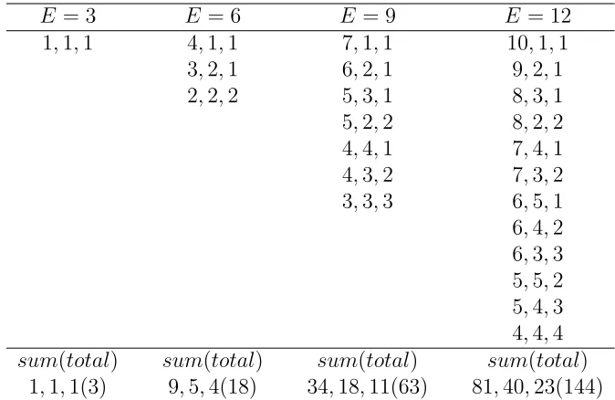
The set of admissible payoff profiles that satisfy these bounds is uncountable. This as-pect leads to some technical issues that are addressed later. Table 1 presents the (unit) discretized set of admissible payoff profiles for n= 3 andE= 3,6,9,12.
9
Axiom 3 (Representativeness). The final allocation is representative if it receives as input every admissible allocation.
Representativeness is framed inside the set of admissible allocations. In technical terms, by representativeness each allocation in this set receives some strictly positive weight.
Equal treatment of allocations - It determines that each admissible allo-cation is equally important. In our setting the equal treatment is over the set of admissible allocations and not over the individuals. There is a duality between individuals and allocations. Intuitively, each allocation could have been legitimately proposed by some individual in some context. Therefore, it is equally weighted - the principle of equal treatment [over proposals].
Axiom 4 (Equal treatment of allocations). The final solution satisfies equal treatment of allocations if every allocation is uniformly weighted.
An equal treatment of allocation proposal removes from the final allo-cation any bias, prejudice, or individual preference that are not founded in the different strategic position of the individuals. Other distributions would have introduced other sort of bias that we cannot justify in general without an underlying theory that supports it.10
4. The description of the procedure
In this section, we describe in detail the construction of our allocation rule. In particular, we describe the mathematical representation of the principles presented in the previous section.
4.1. Continuous versus discrete action space
In a continuous action space, between two admissible allocation profiles that satisfy the bounds in footnote 8 there is an uncountable set of possible allocations. Actually, the meaning of ”between” is not well defined. The
10
E = 3 E = 6 E = 9 E = 12 1,1,1 4,1,1 7,1,1 10,1,1 3,2,1 6,2,1 9,2,1 2,2,2 5,3,1 8,3,1 5,2,2 8,2,2 4,4,1 7,4,1 4,3,2 7,3,2 3,3,3 6,5,1 6,4,2 6,3,3 5,5,2 5,4,3 4,4,4
[image:10.612.135.472.124.343.2]sum(total) sum(total) sum(total) sum(total) 1,1,1(3) 9,5,4(18) 34,18,11(63) 81,40,23(144)
Table 1: The set of admissible allocation profiles forn= 3 andm= 1,2,3,4.
comparison between two profiles always implies that at least some individual fares better at the expense of another individual. In order to express these concepts mathematically, we consider a discrete action space because it is easier to account for all admissible allocation profiles of definition 1. This set is now countably infinite.11 In other words, we move from the usual
continuous space in which resources and allocations are values in R+, to a discrete space in which resources and allocations are values in N1. Finally, we obtain an asymptotic distribution that is valid in the former space. The discretized set of admissible allocations forn = 3 and E = 3,6,9,12 is given in Table 1.
4.2. The construction of the procedure
We start by considering the following example. Suppose that n = 3 and
E = 3. In a discrete decision space case there is one admissible allocation that simultaneously satisfies axioms 1 and 2, i.e., (1,1,1). The allocations (2,1,0) and (3,0,0) fail the non-zero requirement of axiom 2. However, if
11
E = 6 there are three admissible allocations that simultaneously satisfies axioms 1 and 2, i.e., (4,1,1),(3,2,1) and (2,2,2),see Table 1.
This process of generating admissible allocations can be generalized by letting E =nm, where m = 1,2, ..., and n is the number of individuals (see Remark 1 in the end of this section for a technical explanation).12
Subsequently, for a givennandm,we sum vertically the individuali∈N
payoffs and denote this sum assumn
i (m).At the bottom of Table 1, we show
each individual sum of payoffs over all admissible allocations. Every admis-sible allocation contributes equally for the final allocation, i.e., the principle of representativeness and equal treatment, axiom 3 and 4, respectively. The objective is to find a general expression or recursion that characterizes the sum of the values in the sequence for any m.
In the next step we define the ratio of the individuali sum of admissible payoffs, with respect to the total, i.e.,
rin(m)≡sumni (m)/Xn
k=1sum
n k(m).
The result is the share of individual i on the total resources. Finally, we consider the limit of rn
i (m) form ↑ ∞.
For instance, in Table 1 the individual 1 ratio grows from r13(1) = 1/3
for m = 1 to r3
1(4) = 81/144 for m = 4. For m ↑ ∞, the individual 1 ratio
converges tor3
1 ≡r13(∞) = 11/18 (see Proposition 1 below). In other words,
our allocation rules states that the individual located farthest upstream must receive 61.1(1)% of the total resource under dispute. Formally,
Definition 2. The individual i∈N asymptotic allocation is defined as
φni ≡rinE ≡ lim
m→∞
sumn i (m) Pn
k=1sumnk(m)
E, (1)
where rn
i represents the asymptotic share of the total resource.
Note the compromise between cooperative (preferred by the individuals located the farthest downstream) and non-cooperative behavior (preferred by the individuals located the farthest upstream). For instance, if E = 9 (see Table 1), we are considering admissible allocations that can be regarded
12
as the result of a more cooperative motivated agreements, i.e., (3,3,3) or (4,3,2), and admissible allocations that seem to be the result of a more non-cooperative motivated agreement, i.e., (7,1,1) or (6,2,1). In between, there are admissible allocations that may not fall in any of these two extreme cases, i.e., (5,3,1), (5,2,2) and (4,4,1).
Note that as m ↑ ∞ (or equivalently, as E ↑ ∞), the discretization be-comes finer and vanishes. Therefore, we consider every admissible allocation profile that could possibly be built with a continuous action space.
Recall that we started the discussion justifying the passage from a con-tinuous to a discrete consumption space. Now, asymptotically, we move back from the discrete to the continuous space to obtain a unique distribution.
Remark 1. We considerE =n,2n, ..., mn, ...,(forE < nthe admissible set is empty) instead of E = 1,2, ..., k, .... Asymptotically, for m ↑ ∞ or k↑ ∞,
both approaches are equivalent. The chosen approach simplifies the compu-tation of the general expressions that characterize the sum of each individual payoff as a function of m.
5. The Allocation Rule
Our ultimate objective is to obtain a general expression for the total resource asymptotic share φn
i of individual in positioni∈N as a function of
the total number of individuals n.
Proposition 1. The admissible asymptotic allocation is,
φni = 1
nE
Xn
k=i
1
k, (2)
for i= 1, ..., n and n= 1,2, ....
The contribution and equal weight of every allocation that can be de-fended as a possible final agreement (admissible allocation) are some strong points of our allocation rule. The obtained solution is also unique and ana-lytical which is of great relevance for applied work.
φn
i, is then the sum of all feasible values. For instance, in a n = 3 problem,
the individual i = 1 can be located first, second or third, with respective values, 1, 1/2 and 1/3.However, the individual i= 2 cannot be located first because individual i = 1 would not allow it. Consequently, the individual
i = 2 can be located second or third, with respective values, 1/2 and 1/3.
Finally, individual i = 3 has no other possibility than being always in the third position which has a value of 1/3.
There is also an intuitive relation between the allocation proposed in (2) and the Shapley (1953) value of a particular TU game. This issue is discussed in the following Section.
Some comments on empirics
Contrary to most of the literature in allocation problems that focus on welfare or other maximizing objectives, we have a general agreement and easy application objective. Therefore, if the proposed allocation rule replicates av-erage or representative human behavior, even in very challenging and subtle situations, then it is more likely that our consensus objective is reached. In this respect, our results coincide with some controlled experiments and empirical studies.
For instance, in the casen = 2 our admissible asymptotic allocation is,
φ2 = (3/4,1/4)E. (3)
Engel (2011) aggregates information of 129 published papers on the dictator game and found that dictators on average keep a share of 71.65%, which is close to the 75% proposed by our allocation rule. Other papers predict similar values depending on the treatment.
In the case n= 3 our admissible asymptotic allocation is,
φ3 = (11/18,5/18,2/18)E. (4)
offer of individual 2,as a percentage of the offer of individual 1, was around 40%, in the former and around 30%, in the latter case. Our allocation rule predicts 40% of the individual 1 offer.
6. Properties of the Allocation Rule
In this section, we show that the proposed solution satisfies a set of de-sirable properties.
P1: (monotonic decreasing allocation share with i) φn
i > φni+1, for
i= 1,2, ..., n−1.
It is the most natural property. The higher the individual in the stream, the larger is its share on the total resource. This property is connected with the strategic advantage principle of axiom 1.
P2: (monotonic decreasing allocation share with n) φn
1 > φn1+1 and
φn
i > φni+1+1, for i= 1,2, ..., n.
The first part, i.e., φn
1 > φn1+1, states that the allocation to the most
upstream individual, i= 1,decreases as the number of individuals increases. This property should be natural for every individual allocation. However, for the other downstream individuals there is some ambiguity in the comparisons. The addition of one or more new individuals may change the ordering which has strategic implications. For instance, consider the individual i = 3 in
n = 3. If we add a new individual inew the allocation share of individual i
is going to depends crucially on the position that this new individual will occupy in the sequence. If this new individual is positioned at inew ≤3 then
individual i is pushed to the fourth position (i.e., it becomes i = 4) and consequently obtains a lower allocation share. This is what the second part (i.e., φn
i > φni+1+1) of property P2 says; there exists a monotonic decreasing
relation with n in the downward diagonal. Table 2 provides a numerical illustration. Otherwise, if the new individual is positioned at inew = 4, then
n = 2 n= 3 n = 4 n= 5 n = 6
i= 1 0.75000 0.61111 0.52083 0.45666 0.40833
i= 2 0.25000 0.27777 0.27083 0.25666 0.24166
i= 3 0.11111 0.14583 0.15666 0.15833
i= 4 0.06250 0.09000 0.10277
i= 5 0.04000 0.06111
[image:15.612.161.453.123.229.2]i= 6 0.02777
Table 2: Individual asymptotic shares of the total endowment forn= 2,3,4,5,6.
Therefore, careful should be taken when transposing properties standard in static to sequential settings. Not always exist an immediate analogous between these two worlds because of the different strategic considerations.
P3: (monotonic decreasing relative share withi)φn
i/φni+1 > φni+1/φni+2,
for i= 1,2, ..., n−3.
The result states that the individual i allocation is not only larger than that of individual i+ 1 (see property P1) but it is also larger in relative terms than the one thati+ 1 obtains with respect toi+ 2.While in absolute terms the individuals’ allocations decrease as we move downstream, in rela-tive terms they decrease less for the most downstream individuals. In other words, as we move from i = 1 to i = n, the allocation share decreases in a convex fashion. This property favors equity and it is related with property
P6 below.13
P4: (individual n weak relative share) φn
n−2/φnn−1 < φnn−1/φnn.
The monotonic relation ofP3 is not true for the last individual compar-ison. The relative share of individual i = n − 2 over i = n − 1 is lower than the relative share of individual i = n−1 over i = n. This is because individual i = n is the last in the sequence, therefore, in a weak strategic position. There are two factors that play a role in each individual allocation. The first is the equity concerns of the other individuals. The second is the
13
strategic position of each individual with respect to the next one. The last individual in a sequential allocation problem does not benefit from the latter effect. Virtually, it has no strategic influence. For that reason, its allocation falls relative to the allocation of individual i=n−1.14
0.0 0.2 0.4 0.6 0.8 1.0
0.0 0.2 0.4 0.6 0.8 1.0
Cumulative share of individualsHlowest to highest allocationL
Cum
ula
tiv
e
sha
re
of
the
alloc
[image:16.612.188.424.189.428.2]ation
Figure 1: Lorenz curve. perfect equality curve (blue), n= 2 (red),n= 3 (brown),n= 4 (green).
P5: (monotonic decreasing relative share withn)φn
i/φni+1 > φni+1/φni+1+1,
for i= 1,2, ..., n−1.
Similar to property P3, as the number of involved individuals increases, the relative share, measured by the ratio between allocations decreases, in particular for the most upstream individuals.
P6: (Lorenz inequality increases with n)
14
The equity concerns of the other individuals toward individuali= 1 is negative and equals to−(1−φn
1),while the strategic positioning value is maximal and equal to 1.On the
other hand, the strategic positioning value of individualnis minimal and equals to 0,but benefits from positive equity concerns, which has a value ofφn
n. The distinction between
Figure 1 illustrates this property. As the allocation shares are being adjusted for the increasing number of individuals and everybody tends to obtains less, see property P2,it follows that the more upstream individuals’ concessions to the more downstream ones decreases in relative terms. In other words, the most upstream individuals accept a reduction of their share when the number of individuals increase but this concession decreases in relative terms. Consequently, we observe an increase in inequality in Lorenz terms.
We must also note the directional interpretation of this property. For instance, if instead we consider a decrease in the number of individuals then we observe a decrease in Lorenz inequality which would be accepted as pos-itive. Consequently, what the property is actually stating is that it is more difficult to obtain equitable agreements (in Lorenz sense) in larger than in smaller groups.
Finally, we acknowledge the importance of equity. However, it may be a utopic objective. If we constraint the allocation design on this objective, ignoring the positional advantage of the most upstream individuals, then we would have failed with the objective of presenting a practical and realistic solution to be accepted by the involved parties.
P7: (Lorenz geometry)
The edges of the n-Lorenz curve are tangent to the n−1-Lorenz curve, and so on. Figure 1 illustrates this property. Under some conditions, it is an alternative method of obtaining expression (2).
P8: (Shapley value from equal division): The admissible asymptotic allocation is the Shapley value of a particular TU game.
This property establishes the connection between the allocation proposed in (2) and the Shapley (1953) value of a particular TU game with a structure similar to an ordered cost allocation problem, e.g., the airport problem (Lit-tlechild and Owen, 1973; Thomson et al., 2007).15 As an illustration of such
coalition game, suppose that the allocation (E/3, E/3, E/3) is temporally agreed upon between n = 3 individuals ordered sequentially. Then, we can
15
consider what each coalition can achieve by deviating from this agreement. Individual 1 on the upstream can deviate and obtain the full resource, i.e.,
v({1}) =E.However, if individual 1 follows the agreement and getsE/3, in-dividual 2 can deviate to obtain the remaining resource, i.e., v({2}) = 2E/3.
On the other hand, the individual 3 cannot get more than v({3}) = E/3 which only happens if all the other individuals follow the agreement. Sim-ilarly, the coalition between individual 1 and 2 can get the full resource, i.e., v({1,2}) = E. The same happens to the coalition between individual 1 and 3. However, the coalition between individual 2 and 3 can get at most
v({2,3}) = 2E/3 if individual 1 follows the initial equal split agreement. The grand coalition formed by all individuals worth v({1,2,3}) = E. It is easy to show that for the coalition game just described the Shapley value coincides with the allocation proposed in expression (2), see Table 2. This construction can be generalized for arbitrary n.16
In this sense, the proposed allocation can be called the ”Shapley value from equal division” in just the same way as the ”Walrasian allocation from equal division” (Thomson and Varian, 1985). This property is relevant be-cause it links our seemingly unrelated approach and the Shapley value re-sulting from a particular airport problem. Intuitively, our approach averages over the set of admissible allocations while the Shapley value averages over the marginal contributions of individual players across all different orderings of coalition formation, see Footnote 10 above. Moreover, the observed rela-tion suggests that for each variarela-tion of our original model (see Secrela-tion 7) it may exists a particular TU game for which the Shapley value coincides with the solution obtained through our approach.
Consistency and other comments
We have presented and discussed a set of properties associated with the allocation rule proposed in (2). We now consider consistency (Thomson, 2011; Moulin, 2000; among others). In our sequential setting an equal relative treatment among neighbor individuals seems to be a natural consistency requirement.
16
In spite that the Shapley value and our approach agree for the described game, there is no immediate link between the marginal contribution of each different sized coalition with each term in the summationPn
k=i1/k of expression (2) in a general and meaningful
We motivate consistency in relative terms as follows. Suppose thatn = 3,
and note that individual 1 keeps the amount φ3
1 of the available resource E
and passes the remaining to individual 2, subsequently, individual 2 keeps the amount φ3
2 of the available resource E −φ31 and passes the remaining
to individual 3. In our setting, consistency means that in relative terms, individual 3 should be treated in the same way by individual 2 as individual 2 is treated by individual 1. In other words, it imposes thatφ3
1/φ32 =φ32/φ33.
Simultaneously, the allocation must be efficient, i.e., φ3
1+φ32+φ33 =E.
Definition 3 (relative consistency). An allocation rule is consistent in relative terms ifφn
i/φni+1 =φni+1/φni+2and
Pn
i=1φniE =Efori= 1,2, ..., n−2.
As defined, consistency is related with propertyP3 above. Consequently, the allocation rule proposed in (2) does not satisfy this definition of consis-tency. Other interpretations of consistency are possible.
Herings and Predtetchinski (2012) propose an allocation rule that applied in our setting is given by:
φn
i =δi−1/ Xn
k=1δ
k−1,
whereδ∈(0,1) is a common discount factor. We can show that their sharing rule does not satisfy propertiesP3, P4 andP5.The relative bargaining power is constant for varying i and n. An implication is that, on the contrary to our allocation proposal their rule satisfies our definition of consistency.
However, we note that in sequential allocation problems of the kind pre-sented in the current paper, consistency imposes that pairwise allocations must be linked in a predetermined (linear) order, which is mathematically convenient in some class of allocation problems, as for instance bankruptcy problems, see Thomson (2003). Moreover, there is not a unique definition of consistency.
7. Extensions
This paper is the first step in a new class of allocation rules for sequential problems. We have presented the approach that we consider to be the most focal. However, our theory is particularly flexible, the reader is free to redefine the admissible set or to reinterpret the concepts in the axioms 3 and 4, see Footnote 9.
We now consider possible extensions associated with relaxations of axioms 1 and 2, used to define the admissible set of Definition 1. Other extensions associated with variations of the original sequential allocation problem (non-constant resources, unequal weights, asymmetric individuals, satiation levels, etc.) are also possible.
1) One possibility is to keep axiom 2, but replace axiom 1 by its strict version. In other words, an individual located upstream must have a strict advantage over an individual located downstream.
Axiom 5 (Strict Strategic Advantage). If i < j then ci > cj for all
i, j ∈N.
2) The reverse possibility is to maintain axiom 1 but replace axiom 2 by its relaxed version. In this case, allocation profiles in which one or more individuals obtain a zero payoff are possible.
Axiom 6 (Non-Strict Payoff Right). ci ≥0 for all i∈N.
3) We can also consider the strict version of axiom 1 and the relaxed version of axiom 2 simultaneously, i.e., replace these by axioms 5 and 6, respectively.
that are less equitable in Lorenz sense.17’18 In order to see it, consider the
following example.
Example 1. Let n = 3 and m = 2. Under axioms 1 and 2 the admissi-ble set is: (4,1,1), (3,2,1) and (2,2,2). The respective vector of individual shares is: r3(2) = 1
18(9,5,4). In case 1) the admissible set is composed
by a single profile, i.e., (3,2,1). The respective vector of individual shares is: r3(2) = 1
18(9,6,3). In case 2) the admissible set is: (6,0,0), (5,1,0),
(4,2,0), (4,1,1), (3,3,0), (3,2,1)and (2,2,2). The respective vector of in-dividual shares is: r3(2) = 1
18(11.6,4.7,1.7). In case 3) the admissible set
is: (5,1,0), (4,2,0) and (3,2,1). The respective vector of individual shares is: r3(2) = 1
18(12,5,1).
From the example, it is clear that the individual 3 share of the total re-source [in cases 1), 2) and 3)] is always smaller with respect to the admissible set defined in Section 3, see Table 1. The opposite conclusion holds for indi-vidual 1,which never gets into a worse situation. Mixed results are observed for individual 2 (see the discussion after property P2). These conclusions remain valid for larger values of m, in particular for m ↑ ∞.
A Note for Practitioners
Some situations may justify that prior to the distribution of the total resource among the involved parties; every individual receives a minimum
17
In the casen= 2 the asymptotic distribution remains the same as in 3. For isntance, if axiom 1 is replaced by axiom 5, we simply remove the payoff profile (m, m) from the admissible set, which appears only once for anym.If axiom 2 is replaced by Axiom 6, we add the payoff profile (2m,0). Asymptotically, a single term is irrelevant. However, for n≥3 we must have different asymptotic distributions, because the removed and/or added allocation profiles increase withm.
18
amount. For instance, in a river sharing problem, observations of this kind make sense when a minimum flow is required to keep the habitat of certain species protected. Therefore, from the total river flow, only a part of it can be used for consumption. The asymptotic allocation of Proposition 1 can be straightforwardly applied to these situations in which a part of the resource is equally split or distributed according to other procedures. When justified, this kind of procedure may allow distributions that are less asymmetric and more equitable.
Acknowledgements. We would like to thank Sebastian Cano, Jos´e-Manuel Gim´enez-G´omez, Susan Glazer, Wesley Hurt, Juan Pablo R´ıncon-Zapatero, Neil Sloane and Yves Sprumont for their very useful comments. The usual caveat applies. Financial sup-port from Universitat Rovira i Virgili, Ministerio de Ciencia e Innovaci´on under project ECO2011-24200 and the Barcelona GSE is gratefully acknowledged.
Appendix
Proof of Proposition 1.
The strategy of the proof is the following. We start by constructing the general expression associated with a given sequence of numbers to obtain the respective asymptotic ratio for n = 2,3,4. Finally, using the obtained information we construct an algorithm that delivers the asymptotic allocation for any i and n.
Consider n = 2 and let the resource be E = 2m for each m = 1,2, ...,
and i = 1,2. We sum all admissible payoffs until a pattern emerges for each individual sum. The sequence 2, 8, 18, 32, 50,72, ..., that represents the aggregate sum of payoffs over all agents and profiles has the general expression 2m2.The sequence 1,5,12,22,35...,that represents the individual
1 sum of payoffs over all profiles has the general expression sum2
1(m) =
m(3m−1)/2. Therefore, by (1) the asymptotic share of the total resource is,
r12(m) = m(3m−1)/2(2m2)→3/4.
The sequence 1, 3, 6, 10, 15, ..., that represents the individual 2 sum of payoffs over all profiles has the general expression sum2
2(m) = m(m+ 1)/2.
Similarly, the asymptotic fraction of the total endowment is r2
2(m)→1/4.
Now considern = 3 and let the resource beE = 3m for eachm = 1,2, ...,
The set of admissible allocations for n = 3 and m = 1,2,3,4, is given in Table 1. The aggregate sum of payoff profiles for each individual is shown in the last row. The general expression for the sequence 3,18,63,144,285, ...,19
that represents the aggregate sum of payoffs over all agents and profiles is
sum3(m) = 3m m2−
m2/4
= 18m3+ 3m(1−(−1)m)
/8,
where ⌊.⌋ denotes the floor function. The expression for the sequence 1, 9,
24, 81, 163, 282, ..., that represents the individual 1 sum of payoffs over all profiles is
sum31(3, m) = 3m m2−
m2/4
−Xm
k=1 2k 2−
k2/4
−X⌊(m−1)/2⌋
k=1 (m+k) (m−2k)
= 22m3−6m2−(m+ 1)−(3m−1) (−1)m
/16.
Therefore, by (1) the asymptotic fraction of the total resource is
r31(m) = (22m
3−6m2−(m+ 1)−(3m−1) (−1)m
)/16 (18m3+ 3m(1−(−1)m))/8 →
11 18.
The expression for the sequence 1, 5, 18, 40, 80, 135, ..., that represents the individual 2 sum of payoffs over all profiles is
sum32(m) = Xm
k=1k
2+X⌊(m−1)/2⌋
k=1 (m+k) (m−2k)
= 10m3+ 3m(1−(−1)m)
/16,
and the asymptotic fraction of the total resource is
r23(m) = (10m
3+ 3m(1−(−1)m))/16
(18m3+ 3m(1−(−1)m))/8 →
5 18.
Similarly, the expression for the individual 3 sum sequence 1, 4, 11, 23, 42,
69, ..., is given by,
sum33(m) =Xm
k=1 k 2−
k2/4
= 4m3+ 6n2+ 4m+ (1−(−1)m)
/16,
19
and the asymptotic fraction of the total resource is r3
3(m)→2/18.
Now considern = 4 and let the resource beE = 4m.We proceed form= 1,2, ..., until a pattern emerges. This case is more complex, the expressions
sum4
i (m) for i = 1,2,3,4, are given by non-trivial recursions. The general
expression for the sequence 4,40,180,544,1280,2592, ...,that represents the aggregate sum of payoffs over all agents and profiles is given by the recursion,
sum4[m] = m
m−1sum
4[m−1] (.1)
+4m
2m X
k=0
4m−2−k
2
−k
$
sgn 4m−2−k
2 −k + 2 2 % ,
where sum4[m] = P4
i=1sum4i [m], sum4[1] = 4 and sgn denotes the sign
function. The total number of admissible profiles is sum4[m]/nm. The
ex-pression sum4
1(m) for the individual 1 sum sequence 1, 17, 84, 262, 629,
1289, ..., is given by the recursion,
sum41[m] = sum41[m−1] + sum
4[m−1]
4m−4
+
2m X
k=0
⌊4m
−2−k
2 ⌋
X
l=k+1
(4m−2−l−k)
$
sgn 4m−2−k
2 −k + 2 2 % ,
where sum4
1[1] = 1 and sum4[m−1] is given by (.1). The asymptotic
frac-tion of the total resource is obtained numerically and is given by,
r41(m) =
sum4 1(m)
sum4(m) →
25 48. The expression sum4
2(m) for the individual 2 sequence 1, 10, 46, 141, 334,
680, ..., is given by the recursion,
sum42[m] = sum42[m−1] + sum
4[m−1]
4m−4
+
2m X
k=0
⌊4m
−2−k
2 ⌋
X
l=k+1
l
$
sgn 4m−2−k
2 −k + 2 2 % ,
where sum4
2[1] = 1 and sum4[m−1] is given by (.1). The asymptotic
frac-tion of the total resource is obtained numerically and is
For simplicity, we consider the individual 4 expression sum4
4(m) for the sum
sequence 1, 6, 21,55, 119, 227, ..., which is given by the following recursion,
sum44[m] =sum44[m−1] +sum4[m]/(4m),
wheresum4
4[1] = 1 andsum4[m−1] is given by (.1). Note thatsum44(m) =
Pm
k=1sum4[k]/k. The asymptotic fraction of the total resource is obtained
numerically and is r4
4(m) → 3/48. Finally, the expression sum42(m) for the
individual 3 sum sequence 1, 7, 29, 86, 198, 396, ..., and the asymptotic fraction of the total resource are obtained as the residual difference. In resume, the obtained asymptotic allocation is,
φ4 = (25/48,13/48,7/48,3/48)E. (.2)
The construction of recursions sumn
i (m) for general n are impractical.
In spite of this, using the information obtained so far we are able to derive a general expression for each individual i ∈ N asymptotic allocation. The argument is based in the following general algorithm that reproduces the numbers in (3), (4) and (.2), and consequently for any n.For the casen = 2,
we have c1 ∈ [E/2, E) and c2 ∈ (0, E/2], and by efficiency c1 +c2 = E.
Since asymptotically we consider every admissible allocation in a continuous space we can think as if 1/2 of the allocations have associated a high value to individual i = 1, say c1 = E, and a low value to individual i = 2, say
c2 = 0 by efficiency. The other 1/2 of the allocations give an equal value to
both individuals, say c1 = c2 = E/2. Therefore, by uniform continuity [and
axioms 3 and 4], the mean allocation for individual i= 1 can be written as,
φ21 = (E)/2 + (E/2)/2 = 3E/4,
and by efficiency φ2
2 = E/4, as stated in (3). The same reasoning applies to
the case n = 3, in which c1 ∈ [E/3, E), c2 ∈ (0, E/2) and c3 ∈ (0, E/3],
and by efficiency c1+c2+c3 =E. Therefore, we can think as if 1/3 of the
allocations have associated an high value to individuali= 1,sayc1 =E,and
a low value to individuals i= 2,3, say c2 =c3 = 0, by efficiency. Other 1/3
of the allocations have associated a medium value to individuals i= 1,2,say
c1 =c2 =E/2, and a low value to individuali = 3, say c3 = 0 by efficiency.
The last 1/3 of the allocations give an equal value to all three individuals, say
c1 =c2 =c3 =E/3.Again, applying uniform continuity, the mean allocation
for individual i= 1 can be written as,
for individual i= 2 can be written as,
φ32 = (0E)/3 + (E/2)/3 + (E/3)/3 = 5E/18,
and by efficiency φ3
3 = 2E/18, as stated in (4). For n = 4, in this case,
c1 ∈ [E/4, E), c2 ∈ (0, E/2), c3 ∈ (0, E/3) and c4 ∈ (0, E/4], and by
efficiency c1 +c2 +c3+c4 = E. Briefly, the mean allocation for individual
i= 1 is,
φ41 = (E)/4 + (E/2)/4 + (E/3)/4 + (E/4)/4 = 25E/48,
for individual i= 2 is,
φ42 = (0)/4 + (E/2)/4 + (E/3)/4 + (E/4)/4 = 13E/48,
for individual i= 3 is,
φ43 = (0)/4 + (0)/4 + (E/3)/4 + (E/4)/4 = 7E/48,
and by efficiency φ4
4 = 3E/48, as stated in (.2). Therefore, for n we have,
c1 ∈ [E/n, E), ci ∈ (0, E/i) for i ∈ {2, ..., n−1}, cn ∈ (0, E/n], and by
efficiency Pni=1ci = E. The mean allocation for individual i = 1 is φn1 =
Pn
k=1(E/k)/n, for individual i = 2 is φn2 =
Pn
k=2(E/k)/n, for individual
i = 3 is φn
3 =
Pn
i=3(E/k)/n, and so on. Therefore, for general i and n we
have (2).
References
Adams, J. S., 1963. Toward an understanding of inequity–journal of abnormal and social psychology. Washington: American Psychological Association.
Ambec, S., Dinar, A., McKinney, D., 2013. Water sharing agreements sustainable to re-duced flows. Journal of Environmental Economics and Management 66 (3), 639–655.
Ambec, S., Ehlers, L., 2008a. Cooperation and equity in the river sharing problem. London: Routledge.
Ambec, S., Ehlers, L., 2008b. Sharing a river among satiable agents. Games and Economic Behavior 64 (1), 35–50.
Ansink, E., Weikard, H.-P., 2012. Sequential sharing rules for river sharing problems. Social Choice and Welfare 38 (2), 187–210.
Bahr, G., Requate, T., 2014. Reciprocity and giving in a consecutive three-person dictator game with social interaction. German Economic Review 15 (3), 374–392.
Bonein, A., Serra, D., et al., 2007. Another experimental look at reciprocal behavior: indirect reciprocity. MPRA Paper (3257).
Camerer, C., 2003. Behavioral game theory: Experiments in strategic interaction. Prince-ton University Press.
Camerer, C., Thaler, R. H., 1995. Anomalies: Ultimatums, dictators and manners. The Journal of Economic Perspectives 9 (2), 209–219.
Carraro, C., Marchiori, C., Sgobbi, A., 2007. Negotiating on water: insights from non-cooperative bargaining theory. Environment and Development Economics 12 (02), 329– 349.
Charness, G., Sutter, M., 2012. Groups make better self-interested decisions. The Journal of Economic Perspectives 26 (3), 157–176.
Dinar, A., Ratner, A., Yaron, D., 1992. Evaluating cooperative game theory in water resources. Theory and decision 32 (1), 1–20.
Engel, C., 2011. Dictator games: A meta study. Experimental Economics 14 (4), 583–610.
Gengenbach, M. F., WEIKARD, H.-P., Ansink, E., 2010. Cleaning a river: An analysis of voluntary joint action. Natural Resource Modeling 23 (4), 565–590.
G¨uth, W., Schmittberger, R., Schwarze, B., 1982. An experimental analysis of ultimatum bargaining. Journal of economic behavior & organization 3 (4), 367–388.
Herings, P. J.-J., Predtetchinski, A., 2012. Sequential share bargaining. International Jour-nal of Game Theory 41 (2), 301–323.
Houba, H., 2008. Computing alternating offers and water prices in bilateral river basin management. International Game Theory Review 10 (03), 257–278.
Kahneman, D., Knetsch, J. L., Thaler, R. H., 1986. Fairness and the assumptions of economics. Journal of business, S285–S300.
Kilgour, D. M., Dinar, A., 2001. Flexible water sharing within an international river basin. Environmental and Resource Economics 18 (1), 43–60.
Moulin, H., 2000. Priority rules and other asymmetric rationing methods. Econometrica 68 (3), 643–684.
Parrachino, I., Dinar, A., Patrone, F., 2006. Cooperative game theory and its application to natural, environmental, and water resource issues: 3. application to water resources. Application to Water Resources (November 2006). World Bank Policy Research Work-ing Paper (4074).
Shapley, L. S., 1953. A value for n-person games. In Contributions to the Theory of Games, volume II, by H.W. Kuhn and A.W. Tucker, editors. Annals of Mathematical Studies (28), 307–317.
Thomson, W., 2003. Axiomatic and game-theoretic analysis of bankruptcy and taxation problems: a survey. Mathematical social sciences 45 (3), 249–297.
Thomson, W., 2011. Consistency and its converse: an introduction. Review of Economic Design 15 (4), 257–291.
Thomson, W., Varian, H., 1985. Theories of justice based on symmetry. Chapter 4. In: Hurwicz, L., Schmeidler, D., Sonnenschein, H. (eds.) Social Goals and Social Organiza-tions: Essays in Memory of Elisha Pazner 126.
Thomson, W., et al., 2007. Cost allocation and airport problems. Rochester Center for Economic Research, Working Paper (538).