On Optimal Non Overlapping Segmentation and Solutions of Three Dimensional Linear Programming Problems through the Super Convergent Line Series

http://www.scirp.org/journal/ajor ISSN Online: 2160-8849

ISSN Print: 2160-8830

On Optimal Non-Overlapping Segmentation and

Solutions of Three-Dimensional Linear

Programming Problems through the Super

Convergent Line Series

Thomas Ugbe

1

, Polycarp Chigbu

2

1_{Department of Statistics, University of Calabar, Calabar, Nigeria}

2_{Deparment of Statistics, University of Nigeria, Nsukka, Nigeria}

Abstract

The solutions of Linear Programming Problems by the segmentation of the cuboidal response surface through the Super Convergent Line Series method-ologies were obtained. The cuboidal response surface was segmented up to four segments, and explored. It was verified that the number of segments, S, for which optimal solutions are obtained is two (S = 2). Illustrative examples and a real-life problem were also given and solved.

Keywords

Average Information Matrix, Experimental Space, Line Search Algorithm, Support Points, Optimal Solution

1. Introduction

Linear Programming (LP) problems belong to a class of constrained convex op-timization problems which have been widely discussed by several authors: see [1] [2] [3]. The commonly used algorithms for solving Linear Programming problems are: the Simplex method which requires the use of artificial variables and surplus or slack variables, and the active set method which requires the use of artificial constraints and variables. Over the years, a variety of line search al-gorithms have been employed in locating the local optimizer of response surface methodology (RSM) problems: see [4] and [5]. Similarly, the active set and simplex methods which are available for solving linear programming problems also belong to the class of line search exchange algorithms.

How to cite this paper: Ugbe, T. and Chig-bu, P. (2017) On Optimal Non-Overlapping Segmentation and Solutions of Three-Dimen- sional Linear Programming Problems through the Super Convergent Line Series. American Journal of Operations Research, 7, 225-238. https://doi.org/10.4236/ajor.2017.73015 Received: January 28, 2017

Accepted: May 21, 2017 Published: May 24, 2017

Copyright © 2017 by authors and Scientific Research Publishing Inc. This work is licensed under the Creative Commons Attribution International License (CC BY 4.0).

http://creativecommons.org/licenses/by/4.0/

Open Access

The line search algorithm, which is built around the concept of super con-vergence, has several points of departure from the classical, gradient-based line series. These gradient-based line series do often times fail to converge to the optimum but the Super Convergent Line Series (SCLS) which are also gra-dient- based techniques locate the global optimum of response surfaces with certainty. Super Convergent Line Series (SCLS) was introduced by [6], and later used by [7] and [8]. [9] modified the Super Convergent Line Series (SCLS) and used it to solve Linear Programming Problems, [10] applied Quick Convergent Inflow Algorithm to solve Constrained Linear Programming Problems on Segmented region, and [11] modified the “Quick Convergent In-flow Algorithm” and used it to solve Linear Programming Problems based on variance of predicted response. In [12], it was verified and established that the best number of segments is two (S = 2) for Linear Programming Problems, four (S = 4) for Quadratic Programming Problems, and eight (S = 8) for Cubic Programming Problems, for non-over- lapping segmentation of the response surface. The above algorithms compared favourably with other Line Search algorithms that utilize the principles of experimental design.

Other recent studies on line search algorithms for optimization problems are: [13] in which a modified version of line search for global optimization was proposed. The line search here uses a technique for the determination of ran-dom- generated values for the direction and step-length of the search. Some numerical experiments were performed using popular optimization functions involving fifty dimensions; comparison with standard line search, genetic al-gorithms and differential evolution were performed. Empirical results illu-strate that the modified line search algorithm performs better than the stan-dard line search and other techniques for three or four test functions consi-dered. [14] focused on line search algorithms for solving large-scale uncon-strained optimization problems such as quasi-Newton methods, truncated Newton and conjugate gradient. [15] proposed a line search algorithm based on the Majorize-Minimum principle; here, a tangent majorant function is built to approximate a scalar criterion containing a barrier function, which leads to a simple line search ensuring the convergence of several classical descent op-timization strategies, including the most classical variants of non-linear con-jugate gradient. [16] presented the fundamental ideas, concepts and theorems of basic line search algorithm for solving linear programming problems which can be regarded as an extension of the Simplex method. The basic line search algorithm can be used to find an optimal solution with only one iteration. [17] presented a performance of a one-dimensional search algorithm for solving general high-dimensional optimization problems which uses line search algo-rithm as subroutines.

2. Preliminaries

2.1. Three Dimensional Non-Overlapping Segmentation of the

Response Surface

The space, _Xˆ _{, (the shape of a cube) is partitioned into subspaces called}

seg-ments. These segments are non-overlapping with common boundaries. The space, _Xˆ_{, is partitioned into S non-overlapping segments as follows:}

In Figure 1(a), the cube (experimental space) is partitioned into two seg-ments, S1 andS2, while in Figure 1(b) and Figure 1(c), the cubes are partitioned

into three and four segments, respectively. From the above Figures and their re-spective segments, support points will be picked to form their rere-spective design matrices. The number of support points per segment, according to [18], should not exceed 1 2p p

(

+ +1

)

1, where p is the number of parameters of the

regres-sion model under consideration. Therefore, p≤ ≤n 1 2p p

(

+ +1

)

1, where n is

(a)

[image:3.595.62.533.286.693.2]

(b) (c)

Figure 1. (a): A vertical line, Ƨ, drawn through the middle of a Cube [Two segments (S = 2)]. (b): A vertical line, Ʈ, and a hori-zontal line, ƥ, draw through the middle of a cube [Three Segments (S = 3)]. (c): A vertical line, Δ, and a horihori-zontal line, Ԓ, drawn through the middle of a cube [Four Segments (S = 4)].

the maximum number of support points per segment. The number of support points per segment as given by [6] is

n

+ ≤

1

N

_k

≤

1 2

n n

(

+ +

1

)

1

, where n is the number of variables in the model, Nk is the number of support points in Nk

seg-ment. The support points per segment are arbitrarily chosen provided they sa-tisfy constraint equations and do not lie outside the feasible region.

2.2. Rationale of the Segmentation

Design matrices are formed from the support points obtained from each of the segments created above. The segmentation of the response surface according to [6] is a rapid way of improving the average information matrix and obtaining the optimum direction vector. This is achieved by obtaining the linear combina-tion of the informacombina-tion matrices from the different segments. The improved av-erage information matrix (resultant matrix) is used to compute the optimum di-rection vector, which locates the optimum didi-rection and the optimizer in a very short period or with one iteration. Without segmentation, information leading to the optimizer would have been obtained from only a fraction of the entire re-sponse surface.

With segmentation, more support points are available at the boundary of the feasible region. [18] [19] [20] have shown that a design formed with support points taken at the boundary of the feasible region is better than any other de-sign with support points taken at the interior of the feasible region.

Theorem: The average information matrix resulting from pooling the seg-ments using matrices of coefficients of convex combination is

( )

T T

1

,

s

n k k k k

k

M ζ H X X H

=

=

∑

Proof:

{

}

T T T T

1 1 2 2

T 1 1

T 2 2

T

diag , , ,

0 0 0 0 , 0 0 S S S S

X X X X X X X X

X X X X X X =       =                

where Hk is the matrix of coefficient of convex combination, X XKT K is the

T T T T 1 1 2 2

1

2 2 2

01 02 0

2 2 2

11 12 1

2 2 2

1 2

2 2 2

01 02 0

2 2 2

11 12 1

0 0 0 0 0 0

0 0 0 0 0 0

0 0 0 0 0 0

0 0

0 0

0 0

s

K K S S

k

s

s

n n ns

s

s

n H H H H H H H H

h h h

h h h

h h h

h h h

h h h

h = = + + +                   =_{  }+ _+ +_{ }                   + + + + + + =

∑

      _                        

 2 2 2

1 hn2 hns

          + + +     

Therefore, T 1

1 0 0

0 1 0

1

0 0 1

s K K k H H =       = =      

∑

      

, since 2 0 1 1 n s ik i k h = = =

∑∑

Therefore,

( )

T T

1 s

n K K K K

k

M ζ H X X H

=

=

∑

3. Methodology

3.1. The Theory of Super Convergent Line Series

3.1.1. Definitions and Preliminaries

The Super Convergent Line Series (SCLS) is defined by [6] as

X

= −

X

ρ

d

_(1.1)

X is the vector of the optimal values,

1 N

m m m X w x

=

=

∑

is the optimal starting points, where wm>0; 1 1 N m m w = =

∑

, 1 1 1 m m N m m a w a − − = =

∑

, T

, 1, 2, , .

m m m

a =X X m=  N

d is the direction vector defined as d MA1

( ) ( )

ζN Z .

−

= _{, where}

( ) (

)

T

0 1

. , , , _n

Z = Z Z  Z is an n-component vector of responses; Z_i = f m

( )

_i , is

the ith row of the average information matrix, MA

( )

ζ

N , where

( )

1

A N

M− ζ is

the inverse of the average information matrix;

ρ

_{is the step-length defined as} min Ti _T i i

C X b

C d

ρ = _ − _

 

 , where d is the di- rection vector; T

i

C

is the vector which represents the parameter of linear

in-equalities; X is the starting point and b_i is a scalar of the linear inequalities;

N

ζ _{is an N-point design measure whose support points may or may not have} equal weights;

Support points are pairs of points marked on the boundary and interior of the partitioned space which are picked to form design matrices;

X is the experimental space of the response surface that can be partitioned

into segments such that every pair of support points in the segment is a subset of X ;

( )

(

T

)

nk k k

M ζ = X X is the information matrix, 1

( )

(

T

)

1 nk k k

M− ζ = X X − is the inverse information matrix;

S1 is segment 1, S2 is segment 2,

( )

det

M

ζ

_nk is the determinant of the information matrix;

Hi is the matrix of the coefficients of convex combination and is defined as

(

1 2 , 1

)

diag , , , , 1, 2, , ;

i i i i n

H = h h  h ₊ i=  k

With i = 1, 2 segments, the coefficients of convex combinations, Hi, of the

segments are:

{

}

133

111 122

1 11 12 13

111 211 122 222 133 233

diag V , V , V diag , ,

H h h h

V V V V V V

 

=  _{+ + +} =

  (1.2)

for the inverse information matrix in segment 1,

{

}

233

211 222

2 21 22 23

111 211 122 222 133 233

diag V , V , V diag , ,

H h h h

V V V V V V

 

= _{ }=

+ + +

  (1.3)

for the inverse information matrix in segment 2,

where V111, V122, V133 are the variances of the inverse information matrix of

seg-ment 1 and V211, V222, V233 are variances of the inverse information matrix of

segment 2, respectively.

The average information matrix, MA

( )

ζ

N , is the sum of the product of the k

information matrices and the k matrices of the coefficients of convex combina-tions, thus

( )

T T

1

;

s

A N k k k k

k

M ζ H X X H

=

=

∑

see [6] (1.4)

Segmentation is the partitioning of the experimental space, X , into segments. Segmentation can be non-overlapping and overlapping, and support points are selected from each segment to form design matrices.

An unbiased response function is defined by

(

1

,

2

)

00 10 1 20 2

f x x

=

a

+

a x

+

a x

(1.5) 3.1.2. Algorithm for Super Convergent Line Series

The algorithm follows the following sequence of steps:

1) Partition the experimental space (Cube) into k=1, 2,,s segments and select Nk support points from the kth segment; hence, make up an N-point design,

( )1 1 2

1 1 2

, , , , , ,

; .

, , , , ,

s n n

N k

k n n

x x x x

N N

w w w w

ζ

=

 

=_{ } =

 

∑

 

 

2) Compute the vectors, X∗,d∗,ρ∗.

3) Move to the point, X∗=X∗−ρ∗ ∗d .

4) Is

X

∗

=

Xf

∗? (where

Xf

∗ is the optimizer of f

( )

⋅ ).

Yes: stop,

5) Identify the segment in which the optimal solution is obtained.

3.2. The Average Information Matrix, the Direction Vector, the

Starting Point and the Step-Length

3.2.1. The Average Information Matrix

The average information matrix, M

( )

ζ

n , is the sum of the product of the k

in-formation matrices, and the k matrices of the coefficients of convex combina-

tions given by

( )

T T

1

,

s

n K K K K

k

M ζ H X X H

=

=

∑

for two segments, the average information matrix is

( )

T T T T 11 21 31

1 1 1 1 2 2 2 2 12 22 32

13 23 33

A N

m m m

M H X X H H X X H m m m

m m m

ζ

∗ ∗ ∗ ∗

    = + _{=  }     .

3.2.2. The Direction Vector

The direction vector defined in Section 3.1.1 is computed as follows:

If f(x) is the response function, then the response vector, Z, is given by

0 1 2 n z z Z z z         =        

 , where

(

)

(

)

(

)

0 12 13 1, 1

1 22 23 2, 2

1,2 1,3 2, 1

, , , ,

, , , ,

, , , .

n

n

n n n n

z f m m m z f m m m

z f m m m

+ + + + + = = =    

Hence, the direction vector defined in Section 3.1.1 is computed as

( )

0 1 1 2 A N n d d d M Z d

d ζ −         = =          .

By normalizing such that *T *

1

d d = , we have

1

2 2 2

1 2

2

* 2 2 2

1 2

2 2 2

1 2 n n n n d

d d d

d

d d d d

d

d d d

   _{+ + +}          = + + +          _{+ + +}        ,

where d0 = 1 is discarded.

3.2.3. Optimal Starting Point

The optimal starting point is obtained from the design matrices of the segments

considered. The optimal starting point defined in Section 3.1.1 is obtained as follows:

1

1 1

1

; 0; 1. , 1, 2, , .

N N

m

m m m m m N

m m

m m

a

X w x w w w m N

w

−

= =

=

=

∑

≥

∑

= = =

∑



T

, 1, 2, , .

m m m

a =x x m=  N

Using a 4-point design matrix, 8 8 1 1 1

1

, m , 1, 2, ,8.

m m m m

m m

a

X w x w m

a

−

− =

=

=

∑

= =

∑



3.2.4. The Step-Length The step-length is defined by

T

T

min i i

i C X b

C d ρ

∗ ∗

∗

 ′ ₋ 

 

=  _′ 

 

 , where

ρ

∗ _{is the optimal step-length and}

d∗ is the

normalized direction vector, T

i

C

is the vector which represent the parameter of

linear inequalities, X∗ is the starting point while bi is a scalar of linear

in-equalities.

4. Results and Discussion

4.1. Comparison of Results Obtained Using the Segmentation

Procedure with Existing

Results in the Literature

Problem 1: [[21], Problem 7.2B, Question 2b, pp. 304] Maximize Z=2x1+x2+2x3

Subject to 4x1+3x2+8x3 ≤12

1 2 3

4x +x +12x ≤8

1 2 3

4x −x +3x ≤8

1, 2, 3 0

x x x ≥

Support points are picked from the boundaries of the partitioned segments (Figure 2) provided they do not violate the constraint equations.

Thus X1=

{

(

0,1, 0 , 0,1,1 , 0, 0,1 , 1 2 , 0, 0 ,

) (

) (

) (

)

, 1 4 , 0, 0

(

)

}

and

(

) (

) (

) (

) (

)

(

)

{

}

2 1, 0,1 , 0, 0,1 2 , 1, 0, 0 , 1,1 2 , 0 , 1,1, 0 , , 1 2 , 0, 0

X =  ,

where X1 and X2 is obtained from S1 and S2 respectively.

Thus, the design and inverse matrices are given as follows (from Figure 2):

1

1 0 1 0

1

1 0 0

2 1

1 0 0

2 1

1 0 0

2

X

 

 

 

 

 

=

 

 

 

 

 

; 2

1 1 1 0

1

1 1 0

2 1

1 0 0

2 1

1 0 0

2

X

 

 

 

 

 

=  

 

 

 

 

 

[image:9.595.209.536.72.575.2]

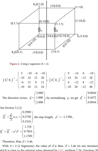
Figure 2. Using 2 segments (S = 2).

(

_T

)

1 1 1

5 10 6 10

10 24 12 20 6 12 8 12 10 20 12 24

X X −

− − −

 

₋ 

 

=

− 

 

−

 

;

(

_T

)

1 2 2

9 14 6 18

14 24 12 28

6 12 8 12

18 28 12 40

X X −

− −

 

_{− −} 

 

=

 − − 

 

− −

 

The direction vector,

2.000

1.000 2.000

d

 

 

=  

 

 

; by normalizing d, we get

0.8944

0.4472 0.8944

d∗

 

 

=  

 

 

,

(See Section 3.2.2)

1

0.2990

0.2758 0.1516

N i i i

X∗ w x

=

 

 

= _{=  }

 

 

∑

, the step-length,

ρ

∗= −1.1396,

1.318

0.7854 1.1709

X∗ X∗

ρ

∗ ∗d

 

 

= − _{=  }

 

 . Therefore, Max Z = 5.46.

With S = 2 (2 Segments), the value of Z is Max. Z = 5.46 (in one iteration) which is close to the optimal value obtained by [21], problem 7.2b, Question 2b, pp. 304, as Max Z = 5.00 (in 3 iterations). The maximum values of Z for this problem using 3 and 4 segments are: 5.81 for (x1, x2, x3) = (1.265, 0.7891, 1.2431),

and 5.77 for (x1, x2, x3) = (1.0008, 0.6606, 1.5523). These values are not optimal

because they do not compare favourably with the existing solution got by [21] using the simplex method.

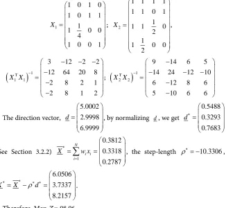
Problem 2: [[22], Ex. 2.4, Q. 14(ii), p. 215] Maximize Z=5x1+3x2+7x3

Subject to x1+x2+2x3 ≤26

1 2 3

3x +2x +x ≤26

1 2 3 18

x +x +x ≤

1, 2, 3 0

x x x ≥

Support points are picked from the boundaries of the partitioned segments (from Figure 3) provided they do not violate the constraint equations.

Thus X1=

{

(

0,1, 0 , 0,1,1 , 0, 0,1 , 1 2 , 0, 0 ,

) (

) (

) (

)

, 1 4 , 0, 0

(

)

}

and

(

) (

) (

) (

) (

)

(

)

{

}

2 1, 0,1 , 0, 0,1 2 , 1,1,1 , 1,1 2 , 0 , 1,1, 0 , , 1 2 , 0, 0

X =  ,

Thus, the design and inverse matrices are given as follows (from Figure 3):

1

1 0 1 0 1 0 1 1

1

1 0 0

4 1 0 0 1

X

 

 

 

=  

 

 

 

 

; 2

1 1 1 1 1 1 0 1

1

1 1 0

2 1

1 0 0

2

X

 

 

 

 

=  

 

 

 

 

,

(

_T

)

1 1 1

3 12 2 2

12 64 20 8

2 8 2 1

2 8 1 2

X X −

− − −

 

₋ 

 

=

 − 

 

−

 

;

(

T

)

1 2 2

9 14 6 5

14 24 12 10

6 12 8 6

5 10 6 6

X X −

−

 

_{− − −} 

 

=

 − 

 

−

 

The direction vector,

5.0002 2.9998

6.9999

d

 

 

=  

 

 

, by normalizing d, we get

0.5488 0.3293

0.7683

d∗

 

 

=  

 

 

(See Section 3.2.2)

1

0.3812

0.3318 0.2787

N i i i

X∗ w x

=

 

 

= _{=  }

 

 

∑

, the step-length

ρ

∗ = −10.3306,

6.0506

3.7337 8.2157

X∗ X∗

ρ

∗ ∗d

 

 

= − _{=  }

 

 

.

Therefore, Max Z = 98.96.

[image:10.595.213.540.183.483.2] [image:10.595.244.505.520.715.2]

With S = 2 (2 Segments), the value of Z is Max Z = 98.96 which is close to the

optimal value (in one iteration) obtained by [22], Ex. 2.4, Q 14(ii), p. 215, as Max Z = 98.80 (in two iterations), using the simplex method. The maximum value of Z for this problem using 3 and 4 segments are: 99.06 for (x1, x2, x3) = (6.0213,

3.725, 8.2537) and 99.15 for (x1, x2, x3) = (6.0746, 3.675, 8.2503).

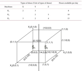
4.2. Illustrative Problem and Application

A producer of leather shoes makes three types of shoes, X, Y and Z, which are processed on three machines, K1, K2 and K3. The daily capacities of the machines

are given in Table 1 as follows.

The profit gained from shoe X is ₦3 per unit, shoe Y is ₦5 per unit and shoe Z is ₦4 per unit. What is the maximum profit for the three types of shoe pro-duced?

Solution: Let X1 be the unit of type X, X2 be the unit of type Y and X3 be the

unit of type Z.

Maximize Z=3x1+5x2+4x3

Subject to 2X1+3X2≤8

2 3

2X +5X ≤10

1 2 3

3X +2X +4X ≤15

1, 2, 3 0

X X X ≥

[image:11.595.208.540.429.716.2]

In a similar manner, the design and inverse matrices are given as follows [from Figure 4].

Table 1. The daily capacity of the machines.

Types of shoes (Unit of types of shoes) Hours available per day

Machines X Y Z

K1 2 3 8

K2 2 5 10

K3 3 2 4 15

Figure 4. Using 2 segments (S = 2).

1

1 0 1 0 1 0 1 1

1

1 0 0

4 1 0 0 1

X       =          

; 2

1 1 1 1 1 1 0 1

1

1 1 0

2 1

1 0 0

2 X         =           ,

(

)

1

T 1 1

3 12 2 2

12 64 8 8

2 8 2 1

2 8 1 2

X X −

− − −   ₋    =  −    −  

;

(

T

)

1 2 2

9 14 6 5

14 24 12 10

6 12 8 6

5 10 6 6

X X −

−   _{− − −}    =  −    −   .

The direction vector,

3 5 4 d     =      

; by normalizing d, we get

0.4243 0.7071 0.5657 d∗     =       , 1 0.3027 0.2953 0.2483 N i i i

X∗ w x

=     = _{=  }    

∑

, step-length

ρ

∗

= −

2.1916

,

1.2326

1.845 1.4881

X∗ X∗

ρ

∗ ∗d

 

 

= − _{=  }

 

 

. Therefore, the maximum value of Z is

₦18.88. This value in one iteration is close to the optimum value got by using the simplex method approach (in three iterations). When 3 and 4 segments were used, the maximum values of Z for this problem are ₦21.25 with corresponding values (X1, X2, X3) = (1.37, 2.08, 1.68) and ₦21.03 with corresponding values (X1,

X2, X3) = (1.43, 2.01, 1.67). These values are not optimal because they do not

compare favourably with the simplex method solution which is Max Z = ₦_18.66.

5. Conclusion

Three dimensional Linear Programming problems have been solved using the line search equation, X∗−ρ∗ ∗d , of the Super Convergent Line Series, by seg-menting the cuboidal response surface into 2, 3 and 4 segments. A real-life problem was also used to achieve the desired result. It was found that the optim-al solution is attained at 2 segments (S = 2) and in one iteration or move even though up to 4 segments (S = 4) were considered. But comparing the solution with the simplex method’s result, a close result was obtained in 2 and 3 itera-tions. Hence, as the name implies, the Super Convergent Line Series (SCLS) lo-cates the optimizer in one iteration and better still with segmentation.

References

[1] Gass, S.I. (1958) Linear Programming Methods and Applications. McGraw-Hill, New York.

[2] Dantzig, G.B. (1963) Linear Programming and Extension. Princeton University Press, Princeton. https://doi.org/10.1515/9781400884179

Press, London.

[4] Wilde, D.J. and Beightler, C.S. (1967) Foundations of Optimization. Prentice Hall Inc., Upper Saddle River.

[5] Myers, R.H. (1971) Response Surface Methodology. Allyn & Bacon, Boston. [6] Onukogu, I.B. and Chigbu, P.E. (2002) Super Convergent Line Series (in Optimal

Design of Experiment and Mathematical Programming). AP Express Publishing, Nsukka.

[7] Chigbu, P.E. and Ugbe, T.A. (2002) On the Segmentation of the Response Surfaces for Super Convergent Line Series Optimal Solutions of Constrained Linear and Quadratic Programming Problem. Global Journal of Mathematical Sciences, 1, 27- 34.

[8] Chigbu, P.E. and Ukaegbu, E.C. (2007) On the Precision and Mean Square Error Matrices Approaches in Obtaining the Average Information Matrices via the Super Convergent Line Series. Journal of Nigerian Statistical Association, 19, 4-18. [9] Etukudo, I.A. and Umoren, M.U. (2008) A Modified Super Convergent Line Series

Algorithm for Solving Linear Programming Problems. Journal of Mathematical Sciences, 19, 73-88.

[10] Iwundu, M.P. and Hezekiah, J.E. (2014) Algorithmic Approach to Solving Linear Programming Problems on Segmented Regions. Asian Journal of Mathematics and Statistics, 7, 40-59. https://doi.org/10.3923/ajms.2014.40.59

[11] Iwundu, M.P. and Ebong, D.W. (2014) Modified Quick Convergent Inflow Algo-rithm for Solving Linear Programming Problems. International Journal of Probabil-ity and Statistics, 3, 54-66. https://doi.org/10.5539/ijsp.v3n4p54

[12] Ugbe, T.A. and Chigbu, P.E. (2014) On Non-Overlapping Segmentation of the Re-sponse Surfaces for Solving Constrained Programming Problems through Super Convergent Line Series. Communications in Statistics—Theory and Methods, 43, 306-320. https://doi.org/10.1080/03610926.2012.661510

[13] Grosan, C. and Abraham, A. (2007) Modified Line Search Method for Global Opti-mization. Proceeding of the 1st Asia International Conference of Modeling and Simulation, Phuket,27-30 March 2007, 415-420.

https://doi.org/10.1109/AMS.2007.68

[14] Andrei, N. (2008) Performance Profiles of Line Search Algorithm for Uncon-strained Optimization. Research Institute for Informatics. Centre for Advance Modeling and Optimization, ICI Technical report.

https://www.ici.ro/neculai/p12a08

[15] Chouzenoux, E., Moussaoui, S. and Idier, J. (2009) A Majorize-Minimize Line Search Algorithm for Barrier Function Optimization. 17th European Signal Proc-essing Conference,Glasgow, 24-28 August 2009, 1379-1383.

[16] Zhu, S., Ruan, G. and Huang, X. (2010) Some Fundamental Issues of Basic Line Search Algorithm for Linear Programming Problems. Optimization, 59, 1283-1295.

https://doi.org/10.1080/02331930903395873

[17] Gardeux, V., Chelouah, R., Siarry, P. and Glover, F. (2011) EM323: A Line Search Algorithm for Solving High Dimensional Continuous Non-Linear Optimization Problems. Soft Computing, 15, 2275-2285.

https://doi.org/10.1007/s00500-010-0651-6

[18] Pazman, A. (1987) Foundation of Optimum Experimental Design. D. Riedel Pub-lishing Company, Dordrecht.

[19] Onukogu, I.B. (1997) Foundation of Optimal Exploration of Response Surfaces. Ephrata Press, Nsukka.

[20] Smith, W.F. (2005) Experimental Design for Formulation (ASA-SIAM Series on Statistics and Applied Probability). SIAM, Philadelphia, ASA, Alexandria, VA. [21] Taha, H.A. (2006) Operations Research: An Introduction. 7th Edition, Macmillan

Publishing Company, New York.

[22] Gupta, P.K. and Hira, D.S. (2008) Operations Research. S. Chand and Company Limited, New Delhi.

Submit or recommend next manuscript to SCIRP and we will provide best service for you:

Accepting pre-submission inquiries through Email, Facebook, LinkedIn, Twitter, etc. A wide selection of journals (inclusive of 9 subjects, more than 200 journals)

Providing 24-hour high-quality service User-friendly online submission system Fair and swift peer-review system

Efficient typesetting and proofreading procedure

Display of the result of downloads and visits, as well as the number of cited articles Maximum dissemination of your research work