Munich Personal RePEc Archive
A generalized panel data switching
regression model
Malikov, Emir and Kumbhakar, Subal C.
Department of Economics, State University of New York at
Binghamton, Department of Economics, St. Lawrence University
28 May 2014
Online at
https://mpra.ub.uni-muenchen.de/56770/
A Generalized Panel Data Switching Regression Model
Emir Malikov∗1,2 Subal C. Kumbhakar1
1Department of Economics, State University of New York at Binghamton, Binghamton, NY 2
Department of Economics, St. Lawrence University, Canton, NY
First Draft: March 20, 2014 This Draft: May 28, 2014
Abstract
This paper considers a generalized panel data model of polychotomous and/or sequential switch-ing which can also accommodate the dependence between unobserved effects and covariates in the model. We showcase our model using an empirical illustration in which we estimate scope economies for the publicly owned electric utilities in the U.S. during the period from 2001 to 2003.
Keywords: Correlated Effects, Multinomial Logit, Nested Logit, Panel Data, Polychotomous, Selection
JEL Classification: C33, C34
∗(Corresponding author)E-mail address: [email protected].
1
Introduction
Sample selection is a common problem in empirical work. Unobserved heterogeneity among units in the data poses a further challenge for practitioners. However, the increased availability of panel data and some recent developments in the literature have alleviated these challenges. In the case of strictly exogenous covariates, Wooldridge (1995), Kyriazidou (1997) and Rochina-Barrachina (1999) offer several ways to tackle both the selectivity and unobserved effects that are allowed to be correlated with covariates in the model. For a comparison of these methods, see Dustmann and Rochina-Barrachina (2007).
The above panel data models, as well as their generalizations that followed later [see Semykina and Wooldridge (2010) and the references therein], largely focus on binary sample selection. How-ever, in many instances researchers face selection (or regime switching) of polychotomous and/or sequential nature. Examples include production technology studies of the industries which contain fully specialized, partly specialized and integrated firms, studies of higher education decisions and many others.
To fill this void, we contribute to the literature by considering a generalized panel data model of polychotomous switching which also allows for the dependence between unobserved effects and covariates in the model. The model we consider can be thought of as a generalization of a standard switching regression model. We show that Wooldridge’s (1995) estimator can be readily extended to the case of polychotomous and/or sequential selection. For consistency, our method requires strict exogeneity of covariates conditional on unobserved effects. We showcase our model using an empirical illustration in which we estimate scope economies for the publicly owned electric utilities in the U.S. during the period from 2001 to 2003.
2
Model
Consider a generalized panel data switching regression model with correlated unobserved effects:
yitr =
(
xritβr+αri +urit if Dit=r
− otherwise (2.1a)
Drit∗=writγrt +ξir+vitr , i= 1, . . . , N; t= 1, . . . , T; r= 1, . . . , R (2.1b) wherexrit andwritare 1×Kr and 1×Lr vectors of exogenous covariates (which may overlap)1 with
corresponding conformable parameter vectorsβrandγrt. (αri, ξir) are individual-specific unobserved effects that are allowed to be correlated with right-hand-side covariates. The outcome variableyr
it is
observed only if the rth regime is selected. The regime selection (switching) is governed by a latent variable Dr∗
it with observable categorical realizations: Dit =r if the rth regime is selected. While
the disturbances ur
it and vitr are orthogonal to (xrit,writ), their distributions are however allowed to
be correlated, namelyE[uritvrit|xrit,witr]6= 0.
We first formalize the regime switching equation (2.1b). For convenience, definexri ≡(xri1, . . . ,xriT) and wri ≡(wr
i1, . . . ,wriT).
Assumption 1. For i = 1, . . . , N, t = 1, . . . , T and r = 1, . . . , R, the conditional mean of unob-served effectsξirin a regime switching equationris a linear projection onwri, i.e.,ξir=L[ξir|wir]+asi,
1
While our model does not require exclusion restrictions and can accommodate the case ofxr
it=w r
it, in practice it is
helpful to have some elements ofwitr excluded fromxrit.
where E[as
i |xri,wri] = 0. The composite error erit ≡ vitr +asi is identically and independently
dis-tributed, conditional on (xri,wri), with the type I extreme value distribution over i. Specifically, we let the linear projection L[ξir|wri] take Chamberlain’s (1980) form, i.e.,2
L[ξir|wir] =wri1δrt1+· · ·+wriTδrtT ≡wriδrt . (2.2) Thus, our model allows for dependence between unobserved effectsξr
i and right-hand-side covariates
writ. This formulation of correlated effects is essentially the one used in (Wooldridge, 1995, p.124).3 One may alternatively permit L[ξir|wri] to take a more restrictive, but parsimonious, specification `
a la Mundlak (1978) which restricts δrt1 =· · · =δrtT (e.g., Semykina and Wooldridge, 2010).4 We
also note that, unlike Wooldridge (1995) who assumes a normally distributed error in the selection equation, we assume the extreme value distribution, which is dictated by a polychotomous nature of the choice set.
The latent variable Drit∗ in (2.1b) can naturally be thought of as measuring an individual’s propensity to select the regimer. Hence, the rth regime is said to be selected if and only if
Dit=r ⇔ Ditr∗> Dj
∗
it ∀ j = 1, . . . , R(j6=r) . (2.3)
While one can treat the regime switching as a system of (R−1) dichotomous decision rules, we follow an alternative approach by considering the former in the random utility framework. That is,
Dit=r ⇔ Ditr∗> max j=1,...,R(j6=r)
n
Ditj∗o . (2.4)
After substituting for Dr∗
it in (2.4) from (2.1b) and making use of Assumption 1, we let ǫrit ≡ max
j=1,...,R (j6=r) n
wjitγjt+wjiδtj+ejito−erit . (2.5)
From (2.5) it then follows that
Dit=r ⇔ ǫrit <witrγrt+wriδrt . (2.6)
Given that erit is extreme value distributed, it follows thatǫrit is multinomial logistically distributed overi with the corresponding marginal distribution Λr(·):
Pr [Dit =r|xri,wri] = Λr(writγrt +wirδrt) =
exp (wr
itγrt+wirδrt) P
jexp
wjitγjt+wjiδjt
. (2.7)
For some strictly positive monotonic transformation Jr(·), condition (2.6) is equivalent to
Dit=r ⇔ Jr(ǫrit)<Jr(writγrt +wriδrt) . (2.8)
We can now look at model (2.1) as a binary selection model, for each given regimer. That is, we can essentially replace the regime switching equation (2.1b) for eachr = 1, . . . , Rwith its equivalent under Assumption 1:
e
Ditr∗= Jr(writγrt +wirδrt)−Jr(ǫrit) , (2.9) 2
Clearly,δr
ttis not identified here.
3
The formulation of equation (2.1b) under Chamberlain’s (1980) specification (2.2) is also equivalent to a reduced form of the followingdynamic regime switching equation: Dr∗
it =ρrDitr∗−1+writγr+vrit.
4
where Der∗
it is a transformed latent variable such that Dit=r if and only if Deitr∗>0, i.e., condition
(2.8) is satisfied. We follow Lee (1982, 1983) and consider Jr(·) ≡ Φ−1[Λr(·)], where Φ(·) is the
standard normal cdf. The advantage of such a transformation is that the random error Jr(ǫrit) in
(2.9) is standard normal by construction, which would later enable us to make use of the truncated moments of the standard normal. Incidentally, the use of Lee’s (1982, 1983) transformation as means of relaxing the normality in the selection equation has also been pointed out but not further developed in the panel data setting by Rochina-Barrachina (1999).
We next formalize the treatment of unobserved effects in the outcome equations of interest as well as the dependence between the two disturbances in (2.1a) and (2.9), where the latter enables us to correct for selectivity bias in the outcome equations.5 For convenience, we defineeǫr
it ≡Jr(ǫrit).
Assumption 2. Fori= 1, . . . , N,t= 1, . . . , T and r= 1, . . . , R: (i) E[ur
it|xri,wri,eǫitr] =E[urit|eǫitr] =L[urit|eǫitr]
(ii) E[αri|xir,wir,eǫitr] =L[αir|xri,wir,eǫitr] .
Assumption 2 states that the disturbance urit is mean independent of (xri,wir) conditional on eǫitr. The latter holds if urit and eǫitr are orthogonal to (xri,wri), a standard assumption made in the sample selection models in the presence of strictly exogenous covariates. Unlike Wooldridge (1995), we also condition the expectation of urit on wri, which is necessary because outcome and selection equations are permitted to have different covariates and non-zero cross-equation correlation between unobserved effects. Further, Assumption 2 does not impose any restrictions on temporal dependence of urit or in the relationship between urit andeǫitr.
We specify the linear projection of urit on eǫitr as
L[urit|eǫitr] =πtreǫitr, (2.10) where πrt is time-varying to allow for temporal dynamics in the relationship between the two dis-turbances. A common alternative to (2.10) is the assumption of bivariate normality of the two errors which also implies linearity of the conditional mean of urit (e.g., Lee, 1983). Our assumption is however less restrictive.
In order to account for correlated effects in outcome equations, Assumption 2 (ii) specifies the structure of unobserved heterogeneity. We follow Wooldridge (1995) and consider the following Chamberlain-type specification
L[αri |xri,wri,eǫitr] =xri1ϕr1+· · ·+xriTϕrT +wi1rωr1+· · ·+wriTωrT +ψtreǫitr
≡xriϕr+wriωr+ψtreǫitr . (2.11) We now derive the selection bias corrected outcome equations. Taking the conditional mean of yitr
from (2.1a) for each regime r, we obtain
E[yitr|xri,wri, Dit =r] =xritβr+xriϕr+wriωr+ (ψtr+πtr)E[ǫeitr|xri,wri, Dit=r]
=xritβr+xriϕr+wriωr+ρrtE[eǫitr|eǫitr <Jr(writγrt +wriδrt) ] , (2.12)
where we have used (2.10) and (2.11) in the first equality, and (2.8) and strict exogeneity of (xr i,wir)
in the last equality. ρrt ≡(ψrt+πrt). Given thateǫitris standard normal by construction, the expected value term in (2.12) equals the negative of the inverse Mills ratio, i.e.,
E[eǫitr|eǫitr <Jr(·) ] =−
φ[Jr(·)]
Φ [Jr(·)]
=−φ[Jr(·)]
Λr(·)
, (2.13)
5
For a counterpart in Wooldridge (1995), see his Assumption 3′on p.126.
where φ(·) is the standard normal pdf.
The model can be consistently estimated in two stages. In the first stage, we estimate γrt
(and δrt) via maximum likelihood as specified in (2.7) performed for each time periodt separately. The obtained estimates γbrt are then used to compute the selection bias correction term. In the second stage, we consistently estimate the main parameters of interest βr via pooled least squares performed on (2.12) that includes predicted inverse Mills ratios (for each regime r, separately). Remark 1. One needs to account for the use of the predicted regressors in the second stage when computing standard errors forβr. Also, it may be of particular interest to conduct inference across equations for different regimes. We suggest following Newey (1984) and casting the model in a multiple-equation system GMM framework which permits the derivation of an asymptotic variance-covariance matrix for our two-stage estimator. Alternatively, paired (nonparametric) bootstrap can be employed.
Remark 2. For expository purposes, the covariates writ and parameters γrt in the regime switch-ing equation (2.1b) are both assumed to be regime-varyswitch-ing. In practice, one needs to impose an identifying restriction on parameters to be regime-invariant for regime-varying covariates unless the latter vary with individuals only. That is, depending on the empirical application, the first stage is to be estimated via conditional, multinomial or mixed logit.
Remark 3. An obvious drawback of the regime switching formulation in (2.1b) is the independence of irrelevant alternatives (IIA) which may be hard to justify in a given application. The latter can be easily relaxed by reformulating the regime switching as a nested (sequential) process. For instance, consider a two-tier regime switching. Redefine equation (2.1b) as6
Ditjr∗ =wj1,itγj1,t+wjr2,itγ2,tjr +ξjri +vitjr , j= 1, . . . , J; r = 1, . . . , Rj
where wj1,it and wjr2,it are partitioned sets of covariates: those varying across the first-tier limbs indexed byj and those varying across the second-tier branches indexed byr, respectively.
Then, make a modified Assumption 1 where (an appropriately defined) vjrit can be assumed to be identically and independently distributed, conditional on (xjri ,wj1,i,w2,ijr), with the generalized
extreme value distribution over i. It is easy to show that the “nested logit” counterpart of (2.7) then takes the following form
Pr [Dit=rj] =
expwj1,itγj1,t+wj1,iδj1,t+̺jIj
PJ m=1exp
w1,itm γm1,t+w1,imδm1,t+̺mIm×
expwjr2,itγjr2,t+wjr2,iδjr2,t/̺j
PRj
k=1exp
wjk2,itγjk2,t+w2,ijkδjk2,t/̺j ,
where Ij ≡ logPRj
k=1exp
wjk2,itγjk2,t+wjk2,iδjk2,t/̺j is the so-called “inclusive value”, and ̺j
is the scale parameter which captures the dissimilarity between second-tier regimes and can be shown to equal 1−Corr[vjrit, vitjk]1/2. For more on the estimation of nested logit models, see Wooldridge (2010). The modified switching regression model can then be estimated under the remaining assumptions in two stages as above.
6
3
Empirical Illustration
To showcase our generalized model, we estimate scope economies for an unbalanced sample of 117 electric utilities owned by local governments in the U.S. in 2001–2003. The data include firms of three types: (i) upstream – utilities that generate electricity, (ii) downstream – utilities that distribute electricity, and (iii) integrated – utilities that both generate and distribute electricity. All power generators use fossil fuel only.
In order to quantify scope economies, we first need to estimate production technologies for the industry. We employ the dual approach and estimate the underlying production technology using the cost function in which all covariates are exogenous as justified by economic theory. Given the nature of product and the government regulation, it is widely accepted that electric utilities treat output quantities, input (and output) prices as fixed.
We define the following two outputs: net electricity generated (y1) and peak demand (y2). The
inputs are physical capital (x1), fuel (x2) and others (x3) (including labor) with the corresponding
vector of prices (w1, w2, w3). Here we opt for a parsimonious specification to avoid multicollinearity
and to conserve degrees of freedom given a small sample size. The price of capital (w1) is the sum of
the interest rate on long-term liabilities and the depreciation rate. We compute the fuel price (w2)
by dividing the fuel expenses by the fuel consumption measured in British thermal units (BTU). We follow Arocena et al. (2012) and proxy the price of other inputs (w3), which includes labor and
other operating expenses, by the state index of average wages for all employees from the U.S. Census Bureau. Lastly, the cost (C) is defined as the sum of capital, fuel and operating expenses, where the latter includes generation, distribution, administrative and general operation and management expenses, customer accounts, customer service and sales expenses.
Given the three types of utilities, not all firms produce both outputs and make use of all three inputs in their operations. The three technological processes can be summarized as follows.
upstream: T1 :{(x1, x2, x3)→y1}
downstream: T2 :{(x1, x3)→y2}
integrated: T3 :{(x1, x2, x3)→(y1, y2)}
That is, there are many observations in the data in which upstream and downstream utilities report zero values for some combination of x2,y1 and y2. The latter is a “zero-value observation”
problem common to studies of electric utilities that estimate a common technology (cost function) for all types of utilities (e.g., Arocena et al., 2012).
However, the assumption of a common technology shared by utilities of all three types is quite unrealistic and unlikely to hold in practice. We relax it by allowing technologies to be type-specific and estimating the cost function for each of the three utility types separately: C1(w
1, w2, w3, y1;β1)
for upstream, C2(w1, w3, y2;β2) for downstream and C3(w1, w2, w3, y1, y2;β3) for integrated firms.
Note that our approach does not suffer from the problem of having to deal with zero-value variables because they do not appear in the equations.
Lastly, we recognize that the utility type is likely to be a product of an endogenous choice made by firms, which we model explicitly. We condition the choice of the utility type on (the log of) regime-invariant total sales (S) and total revenues (R) to capture (exogenous to firms) demand.
We estimate the first stage via multinomial logit, where we restrict γ1t = 0 (upstream type) for the identification. We have explored relaxing the IIA assumption by formulating a (partly degenerate) nested two-tier selection: (i) specialized (upstream/downstream) vs. (ii) integrated utilities. We however have consistently failed to reject the null of multinomial logit, i.e.,̺i =̺ii= 1.
Figure 1: Kernel Densities of Scope Economies Estimates
In the second stage, we use the translog form for the dual cost function, onto which we impose the symmetry and linear homogeneity (by dividing input prices by w3) restrictions. To conserve
degrees of freedom, we define correlated effects in both stages using Mundlak’s (1978) specification, as discussed in Section 2.
We use the fitted generalized model to compute scope economies exhibited in the electric utility industry. Unlike what is customarily done in the literature, we do not compute the statistic at some arbitrarily chosen data point (such as mean or median) but rather compute scope economies using actual data for integrated firms. The observation-specific scope economies are computed as
SE = C
1(w
1, w2, w3, y1;β1) +C2(w1, w3, y2;β2)−C3(w1, w2, w3, y1, y2;β3) C1(w
1, w2, w3, y1;β1) +C2(w1, w3, y2;β2)
. (3.1)
Figure 1 plots kernel densities of the scope economies estimates from our generalized model (solid) as well as of the estimates obtained using two auxiliary (misspecified) models: (i) a model of heterogeneous technologies which estimated separate cost functions but ignores endogenous selection (dashed); and (ii) a model of common technology which fits one cost function for all types of utilities with zero-value observations set equal to 0.0001, as widely practiced in the literature (dot-dashed). The figure suggests that the models that fail to account for technological heterogeneity and en-dogenous switching tend to underestimate scope economies: kernel densities based on both auxiliary models are to the left from that based on our generalized model. We attribute this to selectivity and misspecification biases present in the former models. We also formally test for the presence of endogenous switching via a joint Wald test of H0 : ρr1 = · · · = ρrT = 0 for r = 1,2,3. The
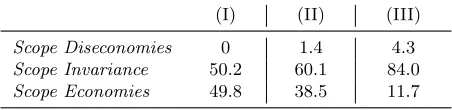
Table 1: Scope Economies Categories, %
(I) (II) (III)
Scope Diseconomies 0 1.4 4.3
Scope Invariance 50.2 60.1 84.0
Scope Economies 49.8 38.5 11.7
NOTE: Model (I) – generalized model of heterogeneous technologies with endogenous selection; Model (II) – aux-iliary model of heterogeneous technologies which ignores selection; Model (III) – auxiliary model of common tech-nology.
of a power generator and a power distributor reduces cost by a median of 31%. The distribution of our estimates is consistent with findings reported in the literature (e.g., Kwoka, 2002).
However, kernel densities of the scope economies estimates in Figure 1 do not account for sam-pling errors associated with the estimation of models. Table 1 reports the breakdown of integrated electric utilities into three categories: Scope Diseconomies (SD), Scope Invariance (SI) and Scope Economies (SE). We classify a utility as exhibiting SD/SI/SE if its scope economies point estimate is statistically less/equal/greater than zero at the 95% significance level. Here we use a bootstrap two-stage, multiple-equation variance-covariance matrix obtained using 9,999 replications.
Based on our preferred generalized model, we find that as many as 50% of integrated electric utilities enjoy scope economies. The cost of the remaining half is invariant to the scope. The two auxiliary models however document a far worse picture, according to which 61% to 88% of integrated utilities exhibit scope invariance or, at worst, significant diseconomies of scope.
4
Conclusion
We consider a generalized panel data model of polychotomous switching which also allows for the dependence between unobserved effects and covariates in the model. We contribute to the literature by extending Wooldridge’s (1995) estimator to the case of polychotomous and/or sequential selec-tion. The model is showcased using an empirical illustration in which we estimate scope economies for the publicly owned electric utilities in the U.S. during the period from 2001 to 2003.
References
Arocena, P., Saal, D. S., and Coelli, T. (2012). Vertical and horizontal scope economies in the regulated US electric power industry. Journal of Industrial Economics, 60(3):434–467.
Chamberlain, G. (1980). Analysis of covariance with qualitative data. Review of Economic Studies, 47(1):225–238.
Dustmann, C. and Rochina-Barrachina, M. E. (2007). Selection correction in panel data models: An application to the estimation of females’ wage equations. Econometrics Journal, 10(2):263–293.
Kwoka, J. E. (2002). Vertical economies in electric power: Evidence on integration and its alterna-tives. International Journal of Industrial Organization, 20:653–671.
Kyriazidou, E. (1997). Estimation of a panel data sample selection model. Econometrica, 65(6):1335–1364.
Lee, L. (1982). Some approaches to the correction of selectivity bias. Review of Economic Studies, 49(3):355–372.
Lee, L. (1983). Generalized econometric models with selectivity. Econometrica, 51(2):507–512.
Mundlak, Y. (1978). On the pooling of time series and cross section data. Econometrica, 46:69–85.
Newey, W. K. (1984). A method of moments interpretation of sequential estimators. Economics Letters, 14(2):201–206.
Rochina-Barrachina, M. E. (1999). A new estimator for panel data sample selection models.Annales
d’Economie et de Statistique, 55-56:153–181.
Semykina, A. and Wooldridge, J. M. (2010). Estimating panel data models in the presence of endogeneity and selection. Journal of Econometrics, 157(2):375–380.
Wooldridge, J. M. (1995). Selection corrections for panel data models under conditional mean independence assumptions. Journal of Econometrics, 68(1):115–132.