Munich Personal RePEc Archive
Derivatives Pricing on Integrated
Diffusion Processes: A General
Perturbation Approach
Li, Minqiang
Bloomberg LP.
8 March 2014
Online at
https://mpra.ub.uni-muenchen.de/54595/
Derivatives Pricing on Integrated Diffusion Processes:
A General Perturbation Approach
Minqiang Li
∗†March 19, 2014
Abstract
Many derivatives products are directly or indirectly associated with integrated diffusion processes. We develop a general perturbation method to price those derivatives. We show that for any positive diffusion process, the hitting time of its integrated process is approxi-mately normally distributed when the diffusion coefficient is small. This result of approximate normality enables us to reduce many derivative pricing problems to simple expectations. We illustrate the generality and accuracy of this probabilistic approach with several examples in the Heston model, including variance derivatives, European vanilla options, timer forwards, and timer options. Major advantages of the proposed technique include extremely fast com-putational speed, ease of implementation, and analytic tractability.
Keywords: Integrated diffusion process; Asymptotic expansion; Hitting time; Derivative pricing; Timer options
JEL Classifications: C02; G12; G13
The contents of this article represent the authors’ views only and do not represent the opinions of any firm or institution.
∗Derivatives Research, Bloomberg LP, 731 Lexington Avenue, New York, NY, 10022. E-mail:
min-qiang.li@gmail.com.
†I thank seminar participants at Bloomberg, Brooklyn College, and Rutgers University for comments and
1
Introduction
There are many financial derivatives whose payoff or pricing is related to an integrated diffusion process. Here by anintegrated diffusion process, we mean a continuous-time stochastic process that is a time integral of a diffusion process. For example, virtually all variance derivative products are associated with the accumulated realized variance, which is often modeled as the time integral of the instantaneous variance for high accumulating frequency. Another example is the continuous-time average price Asian option in which the payoff is a function of the integrated stock process. A third example is interest rate derivatives pricing using short-rate models, in which the integrated short-rate process plays an important role.1
A common technique for pricing derivatives is through solving the corresponding pricing PDE, either analytically or numerically. Financial derivatives related to integrated diffusion processes pose a challenge for this approach. The reason is that the PDE is usually of high dimension. For example, in pricing variance derivatives, in order to form a Markovian sys-tem, one usually has to include simultaneously the instantaneous variance process and the accumulated variance process. Therefore, the pricing PDE also includes both variables. On the other hand, the final payoff of a variance derivative never depends explicitly on the unob-servable instantaneous variance. For example, in the case of a volatility swap, to get the fair volatility swap rate today, we just need to compute the expectation of the square root of the accumulated variance at expiry. If we have the explicit probability density of the accumulated variance at expiry, the computation becomes just a simple one-dimensional integration.
The above discussion highlights the potential usefulness of the probabilistic approach based on the risk-neutral expectation since often fewer variables are involved using this approach than the PDE approach. In practice, however, it is not easy to compute the probability densities. Analytical results are only known for a very limited set of models and even in those cases multiple dimensional Fourier inversion is often involved. Therefore, under many circumstances, in order to use the probabilistic approach effectively, it is useful to have the probability density available through analytical approximation means such as perturbation.
The current paper is one step in this direction. The central object of interest in this paper is the random time that the integrated process first exceeds a fixed budget. We study this hitting time directly rather than the integrated process itself for several reasons. First, for a positive diffusion process, once we have the distribution function of the hitting time, by a duality result, we immediately have the distribution function for the integrated process. Second, a technical but important motivation for the current paper is that the PDEs for functionals of the hitting
1
time are sometimes easier to deal with than those for the integrated process itself. Third, in practice, there are derivative securities whose final payoffs are explicit functions of the hitting time. For example, Soci´et´e G´en´erale Corporate and Investment Banking introduced a new type of variance derivative products called “timer options” in 2007. See Sawyers (2007, 2008). A timer option is similar to a plain-vanilla option, except that it can only be exercised when the accumulated realized variance reaches a given budget. Major banks have since traded timer options. Sawyers (2008) also reports that more complex derivatives with timer features such as timer swaps have been introduced to the over-the-counter derivatives market.
The basic assumption we use is that the diffusion coefficient of the diffusion process is small. We perform an asymptotic perturbation analysis on the moment generating function of the hitting time of the integrated diffusion process. We show that under small diffusion coefficient, the hitting time is approximately normally distributed since its moment generating function has an asymptotic form similar to that of a normal random variable. For many common models including the popular square-root process, the approximate mean and variance can be easily obtained in simple closed form. We also generalize the result to the time integral of functions of diffusion processes. The result of approximate normal distribution is very convenient in approximating derivative prices. We give several examples in the paper using the Heston model, including generic variance derivative pricing, plain-vanilla European-style options, timer forwards, and timer options. In all these examples, the final approximated price is either a simple one-dimensional integration or in closed form. Numerical analysis shows that these approximations are fairly accurate when the volatility coefficient is not too large, in addition to being extremely fast and easy to implement.
There have been studies in the literature on integrated diffusion processes. For example, Dufresne (2001) studies the integrated square-root process. Forde and Jacquier (2010) consider the integrated geometric Brownian motion process to price Asian options. The approach we take here is different. While existing literature focuses mostly on exact properties of specific processes, we study the approximate properties of general integrated processes. These two branches of research directions are therefore complementary to each other.
The use of perturbation technique in derivative pricing has a long history and it is difficult to list all the references. The two references which are most closely related to the current paper are Lewis (2000) and Lipton (2001), where the authors consider volatility of volatility expansion for plain-vanilla European-style option prices in the Heston model. One difference is that in this paper we perform an expansion for the moment generating function of the hitting time of any integrated diffusion process and then use it to price many different derivative products.
methods such as Monte Carlo or PDE. First, the computation usually takes well below one second or even below one millisecond for computing each derivative price, compared with Monte Carlo or PDE which can take many orders of magnitude more computational time. The benefit in computational time is much greater than it first seems when looking at pricing a single option price. Below I elaborate on this point because it is often overlooked and under-appreciated. Take for example, the computation of credit value adjustment (CVA) required by Basel II and III (see, for example, Gregory (2012)). Roughly speaking, CVA is a time-average of conditional exposure up to a future horizon, weighted by the default time probability density. In a Monte Carlo setup, for each future time grid and each realized intermediate state variable configuration, one needs to run a Monte Carlo to get a price as a function of the state variables. These intermediate future prices are in turn fed into the time-averaging formula. The number of simulations needed in such a nested Monte Carlo is the usual number of simulations needed for a single price, multiplied by the number of scenarios (usually taken to be at least 1000, but can require a lot more if number of factors involved is large), and also by the number of time steps (usually taken to be somewhere from 20 to 100). Furthermore, hedging analysis, stress testing, risk analysis, real-time pricing, and greek computations all exacerbate the Monte Carlo simulation burden. For example, to compute the greek gamma through bumping and repricing, one needs to repeat the Monte Carlo simulations three times. Related, the availability of closed-form approximations allows us to examine the price sensitivity to model parameters more easily. For example, suppose one wants to study the price of a certain derivative as a function of the long-run mean and the mean-reverting strength in the Heston model. In a Monte Carlo setup, we can sample 10 different values of the mean and the mean-reverting strength. If each Monte Carlo takes 1 minute which is easily exceeded in the cases of exotic derivatives such as timer options, then we will need 100 minutes of computational time since each parameter combination requires a separate Monte Carlo simulation. To contrast, it usually takes less than one second to compute 1000 prices with an analytic approximation.
make heuristic hedging and other decisions based on this observation.
Third, the approximations developed from the perturbation technique are very easy to implement. As we will see from the examples, most of the approximations involve only a one-dimensional numerical integration on the real line. This is to contrast other numerical methods such as the timer option pricing formula in Liang, Lemmens and Tempere (2011) which is a high-dimensional numerical integration in the complex plane involving complicated functions such as modified Bessel functions. These integrals are often very tricky to evaluate numerically due to oscillatory integrand and slow decaying near ends of integration region. Even without these difficulties, multi-dimensional numerical integration is still very expensive computationally.2 For example, Li (2013) reports a computing time of about 60 seconds for pricing one perpetual timer option. Another alternative, PDE method, also requires a lot of expertise and care, especially when a high dimension is encountered. To contrast, valuing one perpetual timer option using the proposed perturbation technique takes less than 10−4
seconds.
There are limitations with the perturbation technique developed in this paper which a potential user should be aware of. First, only a limited number of models have been solved in this paper, and we have only tested the numerical accuracy in the Heston model for some limited set of parameters.3 The Heston model is used in the testing because it is one of the most popular models for derivatives pricing. Also, while the method applies to generic Heston-like stochastic models, not all models possess simple closed-form formulas. Second, the perturbation technique developed in this paper requires the presence of a small parameter, which might not be available in some real-life applications. Third, other methods such as Monte Carlo might be more versatile in the sense that it is easier to incorporate additional features such as American feature into the pricing engine. However, we believe that these limitations do not diminish the advantages of numerical approximations. It is also our hope that future research will address and overcome some of these limitations.
The rest of the paper is organized as follows. Section 2 develops the approximation for the moment generating function of the hitting time of a general integrated diffusion process. We show that under small diffusion coefficient, the hitting time is approximately normally dis-tributed. Section 3 illustrates the usefulness and accuracy of this probabilistic approach using several examples, namely, generic variance derivatives, European options, timer forwards, and timer options. Section 4 concludes.
2
This is not to say that they are not useful. In fact, they are extremely useful because they can provide definite benchmarks to examine the accuracy of approximations or Monte Carlo.
3
2
Approximating the Hitting Time Distribution
2.1
The Setup
We consider a time-homogeneous one-dimensional diffusion processXt whose dynamics is as
follows
dXt=a(Xt) dt+ηb(Xt) dWt. (1)
Here Wt is a standard Brownian motion. Notice that we have singled out a nonnegative
constant η for the diffusion function and will refer to it as the volatility coefficient. The drift and diffusion functions a(Xt) and b(Xt) are assumed to be functions of Xt only. We
assume that the state space of Xt is (0,∞) and that the process does not explode to either
zero or infinity in finite time. Despite its simplicity, this specification covers many important models in finance, including the Black-Scholes model for stock price movement, the Vasicek and Cox-Ingersoll-Ross models for the short rate movement, and the Heston model for the instantaneous variance movement, among many others.
We use ξt to denote the time-integrated process ofXt, defined as follows
ξt=ξ+
∫ t
0
Xudu. (2)
Here ξ0 = ξ is the value of the integrated process at time 0. We assume that ξ ≥ 0.4
Notice that ξt is nonnegative and increasing in t. As motivated by the reasons listed in the
introduction, the central object of interest is the hitting time τB for the process ξt to hit a
certain level B where B≥ξ. That is,
τB≡inf{t≥0 :ξt=B}= inf
{ t≥0 :
∫ t
0
Xudu=B−ξ
}
. (3)
We are interested in the distribution of the random time τB. Therefore, we consider its moment generating function:
MτB(λ)≡E0
[
eλτBξ0 =ξ, X0 =X]. (4)
We assume that the processXtis such thatMτB(λ) is well-defined and exists for a continuous range of real values ofλ.
4
Since (Xt, ξt) is jointly Markovian which is sufficient to determine whether B is exceeded
or not, MτB(λ) is a function of ξ and X only, and not a function of the current time t. This situation is similar to that of perpetual American options in the Black-Scholes model. Therefore, we let
Π(ξ, X;λ)≡MτB(λ). (5)
For notational ease, we will often omit the parameterλin Π(ξ, X;λ) and just write Π(ξ, X). We can interpret Π(ξ, X) as the price of a zero-coupon timer bond which pays 1 dollar when the budgetB is exceeded with the risk-free rate being constant and equal to−λ.
By the Feynman-Kac theorem applied to the random exit time τB, Π(ξ, X) satisfies the
following partial differential equation
XΠξ+a(X)ΠX +
1 2η
2b2(X)Π
XX+λΠ = 0, (6)
with the boundary condition
Π(B, X) = 1. (7)
In the PDE above, we have used subscripts to denote partial derivatives. For general a(X) and b(X) functions, the above PDE is difficult to solve exactly. Therefore, below we take a perturbation approach.
2.2
The Approximation
We approximate the moment generating function ofτBunder the assumption that the volatil-ity coefficient η is small. Small η expansion is considered for plain-vanilla options in Lewis (2000) and Lipton (2001). In Li and Mercurio (2013a), it is shown that for the Heston model and the 3/2 model,τB is approximately normally distributed for smallη in the sense that the asymptotic expansion of MτB(λ) is exactly in the form of the moment generating function of a normal random variable. Below we show that this is true for any time-homogeneous one-dimensional diffusion process.
We make an important remark that by “smallη” here, we do not require thatη is smaller than 1. Rather, we mean that the effect ofη should be small. This could be measured by the long-run variance of the process Xt, for example. Ifb(Xt) is small, then it is possible that η
is much larger than 1 even though the effect ofηis still very small. It is the effect of η on the variability of the processXt that matters.
It is useful for developing perturbation series purpose to have a constantly zero boundary condition. Therefore, we define the functionp(ξ, X) by
Because Π(ξ, X) > 0, this is well-defined. The quantity p(ξ, X) is actually the cumulant generating function of the random variableτB conditioning on that the current process value
is X and the current integrated process value is ξ. From Equation (6), p(ξ, X) satisfies the nonlinear partial differential equation below
Xpξ+a(X)pX +λ+
1 2η
2b2(X)[p
XX+ (pX)2]= 0, (9)
with the boundary condition
p(B, X) = 0. (10)
The above partial differential equation is exact. We can solve it approximately by asymp-totically expanding inη. It is clear that whenη= 0, we get an ordinary first-order differential equation which can be solved exactly by method of characteristics. This gives us the zeroth-order expansionp0(ξ, X) inη2. The first-order expansion in η2 (second-order in η) can then
be obtained by replacing[pXX+ (pX)2
]
with[p0,XX + (p0,X)2
]
. This second-order expansion ofp(ξ, X) in turn gives a second-order expansion for Π(ξ, X). It turns out that because of the special structure of the PDE forp(ξ, X), the first-order expansion inη2 forp(ξ, X) is actually quadratic inλ, as Proposition 1 below states. This is very interesting because it means that in a certain sense,τB is approximately normally distributed for smallη. This is true regardless
of the functional forms ofa(X) and b(X). A detailed proof is given in Appendix.
Proposition 1. Assume that E0eλτB
, E0[eλτB
τB] and E0[eλτ
B
τ2
B] are finite for some range
of λ values in R containing 0. The moment generating function of τB has the following
asymptotic expansion form
MτB(λ)≡E0eλτ B
=eλ(T0+η2H0)+λ2η2H1+o(η2), (11)
where T0, H0 and H1 are not functions of λ or η.5 Furthermore, T0 ≥ 0 and H1 ≥ 0 with
equality if and only if B =ξ. Therefore, for B > ξ, in the sense above, τB is approximately normally distributed with mean µ and variance σ2, where µ and σ2 are given by
µ=µ(B) =T0+η2H0, (12)
σ2 =σ2(B) = 2η2H1. (13)
5
Explicit expressions for evaluatingT0,H0 andH1 are given in Equations (110), (114) and (115) in Appendix.
However, in practice, it is usually easier to directly solve the PDE perturbatively than to use these integral equations. Once the PDE is solved perturbatively to first order in η2
, we can use Proposition 1 to read off T0, H0 and H1
because by Proposition 1 they are multiplied byλ, λη2
and λ2
η2
We make a few remarks below. First, it is useful to take a look at Proposition 1 for the degenerate case η = 0. In this case, the process Xt evolves deterministically according to
dXt/dt = a(Xt). The time τB to hit the budget B becomes exactly T0 = T0(ξ, X), which
satisfies the first-order PDE below:
XT0,ξ+a(X)T0,X+ 1 = 0, (14)
with the boundary condition
T0(B, X) = 0. (15)
Therefore, the moment generating function MτB(λ) degenerates to that of a Dirac delta function atT0, that is, eλT0. This provides a sanity check for Proposition 1.
The approximate mean µ(B) and variance σ2(B) are functions of B, ξ and X as well as
other model parameters. For notational simplicity, we only emphasize their dependence onB
in Proposition 1. They actually depend on ξ and B through the difference B −ξ, but later on we will always assume without loss of generality that ξ = 0. The quantities µ and σ2
are also approximations in the following sense. If we letm1(ξ, X) and m2(ξ, X) be the true
first and second moments of τB when the initial integrated process value isξ and the initial
state variable value isX, then it is easy to see that they satisfy the following PDEs: (see, for example, Chapter 15 of Karlin and Taylor (1991) for a derivation)
Xm1,ξ+a(X)m1,X +
1 2η
2b2(X)m
1,XX + 1 = 0, (16)
Xm2,ξ+a(X)m2,X+1
2η
2b2(X)m
2,XX + 2m1= 0. (17)
By formally differentiating Equation (6) with respect to λonce and twice and settingλ= 0, we can easily see thatµsatisfies Equation (16) asymptotically to order η2. Similarlyµ2+σ2
satisfies Equation (17) asymptotically.6
In many actual applications, the final payoff of the derivative is a function of ξT instead
of τB. Therefore, it is useful to have an approximation for the distribution function of ξT.
LetFZ(·) denote the distribution function of a random variableZ. For simplicity we assume
without loss of generality thatξ = 0. Then, for T > 0, we can approximate the cumulative distribution functionFξT(x) as:
FξT(x)≡P(ξT < x) = 1−Fτx(T)≈N
(
µ(x)−T σ(x)
)
, (18)
6
In fact, all raw moments and central moments ofτB can be approximated to second order inη in the sense of
where N(·) is the cumulative normal distribution function. The first equality in the above statement is easily seen by noticing the following duality betweenτx andξ
T:
{τx> T}={ξT < x}. (19)
Therefore, we have
P(ξT < x) =P(τx > T). (20)
The last approximate equality in Equation (18) is due to Proposition 1. Although it is difficult to show analytically, for reasonable parameter values we have tried using the Heston model, we always observe numerically that FξT(0
+) = 0, F
ξT(+∞) = 1, and that FξT(x) is monotonically increasing inx. For smallη, the above approximation is very good and captures some important features of the simulated distribution ofξT.
2.3
Examples
The proof in Appendix shows a procedure to computeµ(B) andσ(B) needed in Proposition 1. We first compute the characteristic coordinates, and thenT0,H0andH1 needed forµ(B) and
σ(B) are simply given by integrals. For models with simple a(X) and b(X) functions, the integrals can be performed analytically. We give a few examples below. Readers interested in the details of the calculations are referred to Li and Mercurio (2013a). For simplicity, we assume that currently ξ = 0 so that the quantity B in formulas below should be interpreted as the remaining budgetB−ξ.
Example 1: (Square root process where dV =κ(θ−V)dt+η√V dW)
Here the state variableXtisVt. We will interpretVtas the instantaneous variance as in the
Heston (1993) model. It is worth mentioning that this square-root process is also frequently used to model short rates, as in Cox, Ingersoll and Ross (1985). For notational ease, we will assume that the current time is 0. We use V0 to denote the current instantaneous variance,
which is more natural thanV. By solving the PDE forp(ξ, V) to second order inη, the final
T0,H0 andH1 are given by7
T0 =
1
κlogR, (21)
7
We can also use the integral equations in the Appendix. However, it’s much more straightforward to solve the PDE perturbatively and then eyeball the results to getT0,H0 and H1. We can do it because T0 is multiplied by
λ,H0 is multiplied byλη2 andH1 is multiplied byλ2η2 by Proposition 1. In fact, our implementation to get the
results for the Heston model only takes a few lines of code in Mathematica. The first line solves the zero-order PDE. The built-in function DSolve is perfect for this purpose. The second line solves the first-order PDE in η2
and
H0 =
(R−1)[2R2z2+R(2−5z−2z2)−2−z]
4κ2R2(1 +z)3θ +
3zlogR
2κ2(1 +z)3θ, (22)
H1 =
(R−1)(1 + 2R2z+R(2z−3)) 4κ3R2(1 +z)2θ −
(2z−1) logR
2κ3(1 +z)2θ , (23)
with
R=ez−z0+κB
θ, (24)
z0 ≡
V0−θ
θ , (25)
z≡W(z0ez0 ·e
−κB
θ
)
, (26)
where W(·) is Lambert’s product-log function defined implicitly as x = W(x)eW(x). See
Corless et al (1996) for information on product-log function. We refer readers to Li and Mercurio (2013a) for more details on the derivation of the above formulas.
Since R≥1, T0 is nonnegative. Notice also thatT0 is the implicit solution of
θT0+ (V0−θ)
1−e−κT0
κ =B. (27)
This is exactly the deterministic time when ξT0 =B for η = 0. The easiest way to see that
H1 ≥ 0 is through numerical plotting. A three-dimensional plotting is possible because the
denominators of bothH0 andH1 are positive, and the numerators of bothH0 andH1 can be
[image:12.612.94.533.92.258.2]written as a function of the two variablesz0 andκB/θ.
Figure 1 plots the probability density function and cumulative distribution function ofξT in
the Heston model using our approximation as well as the histogram and empirical cumulative distribution function from Monte Carlo simulation. Here the process ξt is the accumulated
realize variance process. Parameters used here are: V0 = 0.087, κ = 2, θ = 0.09, T = 1.5
years, and η = 0.250. As we see, the approximation is fairly good when compared to the histogram from simulation. Both graphs show almost zero mass in the regionsξT <0.06 and
ξT >0.4, and both are left skewed. The theoretical expectation of ξT is given by
E0ξT =θT+ (V0−θ)
1−e−κT
κ . (28)
Notice that it does not depend on η. With the given parameters, the expectation is about 0.1336. Numerical integration shows that the approximate density gives the expectation ofξT
Example 2: (3/2 model where dV =κV(θ−V) dt+ηV32 dW)
Here the state variable Xt is Vt. See Ahn and Gao (1999) for some univariate analysis
on the 3/2 model. This model has been used to model both short rate and instantaneous variance. In this model,T0,H0 andH1 are given by
T0 =
1
κθlog (
V0+θ(eκB−1)
V0
)
, (29)
H0 =
4V0[1 +(logR−1)R]+θ[−3 + (4−4 logR)R+ (2 logR−1)R2]
4κ2[V
0+θ(R−1)]2
, (30)
H1 =
4R−[3−2 logR]R2−1
4κ3[V
0+θ(R−1)]2
, (31)
withR=eκB.Since R≥1, it is very easy to check that T0 ≥0 and H1 ≥0.
Example 3: (Geometric Brownian Motion where dS = (r−δ)Sdt+ηS dW)
Here the state variable is S. For simplicity, we assume r ̸=δ. The degenerate caser =δ
is simpler and can be solved similarly. We solve the PDE ofp(ξ, S) to second order inη. The functionsT0,H0 and H1 can then be read off as
T0 =
1 ˆ
r logR, (32)
H0 =
Brˆ(Bˆr+ 2S)−2(Bˆr+S)2logR
4ˆr2(Bˆr+S)2 , (33)
H1 =
2(Bˆr+S)2logR−Brˆ(3Brˆ+ 2S)
4ˆr3(Brˆ+S)2 , (34)
whereR= (S+Brˆ)/S and ˆr=r−δ.It is easy to verify thatT0>0 andH1>0 ifB >0.
2.4
A Generalization
We now discuss an interesting generalization of the previous setup.8 The result in this sub-section is not used in the numerical study sub-section, and readers interested in the applications of the previous results can skip this subsection completely.
It turns out that the hitting time of the following integrated diffusion process is also approximately normally distributed (to be shown below):
∫ t
0
f(Xu) du, (35)
where Xt is any diffusion process not necessarily living on (0,∞), and f(·) is any
second-order differentiable function. The only requirement is thatf(·) is positive andXthas a small
8
parameterηin its diffusion function. Such a setup has been considered in Cui (2013). Notice that in this casef might not be one-to-one, and the filtration generated by f(Xu) might be
strictly smaller than that ofXu. One example in point is the Sch¨obel-Zhu (1999) stochastic
volatility model where instead of modeling the instantaneous variance Vt, one models the
“signed volatility”vt (so here Xt≡vtis the state variable):
dSt=rStdt+vtStdWtS, (36)
dvt=κ(θ−vt)dt+ηdWtv. (37)
The “signed volatility”vtfollows an Ornstein-Uhlenbech process and has a state space (−∞,∞).
The instantaneous variance is given by Vt=v2t. The joint state variables are (St, vt). Notice
that vt contains strictly more information than Vt sinceVt does not contain the information
about the sign of vt. In this case, the hitting time of the integrated variance∫0tvu2du(rather
than∫0tvudu) is of interest in finance.
Following Cui (2013), we writef(x) =m2(x) for some function mto emphasize that f is
positive. The integrated process we are interested in is
ξt=ξ+
∫ t
0
m2(Xu)du. (38)
Notice that dξt=m2(Xt)dt. The hitting time τB is the first time a budget B is reached by
theξt process:
τB≡inf{t≥0 :ξt=B}= inf
{ t≥0 :
∫ t
0
m2(Xu) du=B−ξ
}
. (39)
Since (Xt, ξt) is a Markovian system sufficient to determine whether B is exceeded or not,
the moment generating function ofτB is again a function of the current statesξ and X. By Feynman-Kac theorem Π satisfies the slightly more general PDE below:
m2(X)Πξ+a(X)ΠX +
1 2η
2b2(X)Π
XX+λΠ = 0, (40)
with the boundary condition
Π(B, X) = 1. (41)
Whenm(x) =√x, the PDE above reduces to the one in the case we have considered previously. The same method of characteristics we have used in the Proof of Proposition 1 applies with little modification.9 The upshot is that τB is still approximately normally distributed. All 9
Specifically, we need to modifyz to be
z= Φ
(
B−ξ+
∫ X
X∗
m2
(u)
a(u) du
)
three equations in Proposition 1 are still valid. The exact formulas for the mean and variance can be obtained, similar to what we have done in Appendix. However, as we have remarked previously in the footnote, in practice it is much easier to directly perturb the PDE in Equation (40) and read off the functionsT0,H0 and H1 from the results.
In some sense, we have already seen one example in this generalized setup. The 3/ 2-model studied in Example 2 is the reciprocal of the Heston 2-model in Example 1, as can be verified using Ito’s lemma. If we let Xt follow the Heston model, then our generalized
result immediately says that the hitting time of ∫0t1/Xudu is also approximately normally
distributed.
The Sch¨obel-Zhu (1999) model, unfortunately, does not give simple formulas when solving it using our perturbation approach.10 The reason is that in this model we cannot obtain the zeroth-order solution T0 in an explicit form. The instantaneous variance when η= 0 is given
by
Vt=vt2 =
(
θ+ (v0−θ)e−κt)2. (44)
The deterministic timeT0 to reach a variance budget B is the solution of
∫ T0
0
(
θ+ (v0−θ)e−κt)2dt=B−ξ. (45)
Unfortunately, it’s not possible to write T0 as an explicit function of ξ and v0 easily unless
θ= 0, orκ= 0, orv0=θ. All special cases are of considerably less interest in practice. Since
the derivatives ofT0 need to be fed into the first-order perturbed PDE for Π, the lack of an
explicit expression forT0 prevents an explicit formula for Π.
There are, nonetheless, some interesting new models that are explicitly solvable in this generalized setup, and we discuss two of them below. The first model is similar to the Sch¨ obel-Zhu (1999) model, except that the volatility process follows a 3/2-process:
dSt=rStdt+vtStdWtS, (46)
dvt=κvt(θ−vt) dt+ηvt3/2dWtv. (47)
Equation (106) then changes to
m2
(X)zξ+a(X)zX= 0. (43)
Modifications to other equations are straightforward.
10
We emphasize that this by no means implies that our perturbation technique is no longer valid. The procedure still works. The distribution ofτB is still approximately normal. It is just that the generalized versions of Equations
We are interested in the distribution ofτB, which is the first time for the process ∫0tVudu to
exceed the remaining budgetB−ξ. Following the PDE convention, we letv0 =v. The PDE
for its moment generating function Π(ξ, v) is given by
v2Πξ+κv(θ−v)Πv+1
2η
2v3Π
vv+λΠ = 0, (48)
with the boundary condition Π(B, v) = 1. This equation can be solved perturbatively to first order inη2. The functionT
0 can be read off from the zeroth-order solution. It is given by (for
simplicity, we letξ = 0 in the following)
T0= 1
κθlog (
z0(1 +z)
z(1 +z0)
)
, (49)
where
z0 =
v−θ
θ , (50)
z=W(z0ez0 ·e
−κB
θ
)
. (51)
Here W(·) is the product-log function. The functions H0 and H1 can be read off from the
first-order solution inη2 by Proposition 1 and are given by
H0=
(
1 +z(14 +z))log(z0/z)
2κ2(1 +z)4θ
+
(z−z0)
[
−3z0+z
(
5 +z(4 +z) + 24z0+z(17 + 4z)z0−2(8 +z)z02−2z02
)]
4κ2(1 +z)4z2 0θ
, (52)
and
H1=
(
2−z(2 +z))log(z0/z)
κ3(1 +z)4θ2 +
8z(2 +z)z0−12(1 +z)z02+ 8z03+z04−z2(2 +z)2
4κ3(1 +z)4z2 0θ2
. (53)
It can be quickly checked that whenB = 0, H0 =H1 = 0, as we would expect from
Proposi-tion 1.
In the 3/2 model we above, since vtis always positive, the function m2(x) =x2 is
one-to-one. Therefore, another approach we could have taken is to use Ito’s lemma to write down the dynamics ofVtand use the result in Proposition 1.11 This is a valid alternative approach. 11
The dynamics ofVtis given by
dVt=Vt(2κθ−(2κ−η2
)√Vt)dt+ 2ηV5/4
dWtv. (54)
Notice that both the drift and diffusion functions involveη. Also, the drift is not mean-reverting unless 2κ > η2
The current approach of using vt as the state variable is slightly simpler because both the
drift and diffusion functions of Vt involve the parameter η, and therefore the perturbation
usingVt as the state variable is a little bit more involved. In general, however,m2 might not
be one-to-one, and the filtration generated by Xt might be strictly larger than m2(Xt). In
these cases, we will have to use the generalization above and Equation (40) since the filtration generated by m2(Xt) might not be sufficient to determine τB. Below we consider such a
model.
This second model we consider is a “signed” stochastic volatility in the same spirit of Stein and Stein (1991) and Sch¨obel and Zhu (1999). The “signed” volatility vt is modeled as
dvt=κvt(θ2−v2t) dt+ηdWtv, (55)
whereκ >0,θ >0 and η are constant parameters. This process has a state space (−∞,∞). We see that the drift function is positive for very negative vt, and is negative for very
pos-itive vt. Therefore, the process is globally mean-reverting. However, the drift function has
three zeros at −θ, 0, and θ. It has a tendency to return to either −θ or θ when |vt| > θ,
and has a tendency to further drift away from 0 when |vt|< θ. The stationary density of vt
is bimodal with the two modes at −θ and θ. Similar processes have been used to study the bifurcation behavior in nonlinear dynamics.12 Let v
0 = v. If η = 0, the process is always
nonnegative or nonpositive and is given by the solution:
vt=v
√
θ2
v2+ (θ2−v2)e−2κθ2t. (56)
Astgoes to infinity, it either goes to−θorθdepending on the sign ofv. We are still interested in the hitting time of integrated variance process ξt where dξt= v2tdt. The function T0 can
be obtained by solving the following ODE:
v2T0,ξ+kv(θ2−v2)T0,v+ 1 = 0, (57)
with the boundary condition T0(B, v) = 0. Or it can be solved by inverting the relation
∫ T0
0
vu2du=B−ξ. (58)
In any case, the result is given by (for simplicity, we letξ= 0 soB is the remaining budget)
T0 =
1
2κθ2 logR, (59)
12
Readers with a physics background will recognize that the drift is the negative of the gradient of double-well potentialU(r) =κr4
/r−κθ2
r2
where
R ≡ v
2+ (e2κB−1)θ2
v2 . (60)
Notice that R≥1 so T0 ≥0. The functionsH0 and H1 are given by
H0 =
(R−1)((1−R)v2+ (R−2)θ2)+((R−1)v2+θ2)RlogR
4κ2R2v2θ6 , (61)
H1 =
(R−1)(2(1 +R)θ2−(1 + 5R)v2)+ 2R((2 +R)v2−2θ2)logR
8κ3R2v2θ8 . (62)
As a quick sanity check, we see thatH0 =H1 = 0 whenB = 0. The approximate mean and
variance ofτB are then given by the last two equations in Proposition 1.
3
Applications to Derivatives Pricing
In what follows, we consider several examples to illustrate the potential usefulness of the dis-tributional approximation developed in the previous section. We consider a general stochas-tic volatility framework. The types of derivative securities we consider include: a variance derivative whose payoff is a function of the realized variance, plain-vanilla European option, a perpetual timer forward contract, and a perpetual timer option. We reduce the prices of these derivatives to either a simple one-dimensional numerical integration or a closed-form expression. Numerical study using the Heston model is also carried out to demonstrate the accuracy of the approximations.
3.1
Variance Derivatives Pricing
Variance derivatives are derivatives written on the realized accumulated variance, which is usually computed as
N
∑
i=1
[
log
( Sti
Sti−1
)]2
, (63)
whereN is the number of days until maturityT, andStj’s are the stock prices on dayj. Notice that the summation goes from 1 to N since we set TN = T. One standard approach is to
model the underlying and instantaneous variance as following a standard stochastic volatility model in the risk-neutral measureQ:
dSu= (r−δ)Sudu+
√
VuSudWuS, (64)
wherer is the constant risk-free interest rate, δ is the constant dividend yield, and WuS and
WV
u are two standard Brownian motions with a constant correlationρ. The daily accumulated
variance is usually modeled using its continuous counterpart ξt, which is defined as
ξt=
∫ t
0
Vudu. (66)
We are interested in computing quantities of the following form
G=E0[g(ξT)]. (67)
For example, forg(x) =x/T org(x) =√x/T,Gis the annualized variance swap rate or the volatility swap rate. Without loss of generality, we assume thatg(0) = 0. Otherwise, we can always definege(x) =g(x)−g(0) and G=g(0) +E0[eg(ξT)]. We also assume thatg satisfies
suitable integrability and differentiability conditions.
If we assume thatηis small, we can approximate Gusing Proposition 1. After integration by parts, the result is given as a one-dimensional numerical integration
G=
∫ ∞
0
(1−FξT(B))g
′
(B) dB≈ ∫ ∞
0
N (
T−µ(B)
σ(B)
)
g′(B) dB. (68)
Given a stochastic volatility model with drift and diffusion functionsa(V) andb(V), the task is then to compute the approximate meanµ(B) and approximate standard deviationσ(B) of the hitting time in Proposition 1. For the Heston model and the 3/2 model, these expressions can be computed easily fromT0,H0 and H1 given in Examples 1 and 2.
Below we examine the accuracy of the above approximation for the volatility swap rate in the Heston model. That is,g(x) =√x/T. To remove the singularity at B= 0 in g′
(B), it is useful to perform a change of variabley=√B in Equation (68) to get
GApprox=
1 √ T ∫ ∞ 0 N (
T −µ(y2)
σ(y2)
)
dy. (69)
The above approximation is valid for any a(V) and b(V) functions. In our numerical analysis, we consider the popular Heston model. In this model, the volatility swap rate can be computed using the known moment generating function ofξT which provides us a benchmark
to check for accuracy. Specifically, we have
GNI=
1
√ TE0
[√ ξT
]
= 1 2√π√T
∫ ∞
0
1−MξT(−λ)
λ3/2 dλ, (70)
where the subscriptNIstands for numerical inversion, andMξT(−λ) is the moment generating function MξT(−λ) ≡E[e
−λξT
that the usual Laplace inverse transformation will involve contour integration in the complex plane. Equation (70) is very nice because it is an inversion on the real line. This is a well-known result in mathematics and has connections to fractional calculus, see Wolfe (1975). In finance, this inversion trick has been popularized by Sch¨urger (2002) and subsequently by Gatheral (2006), among others. In the Heston model, MξT is given explicitly by (see Cox, Ingersoll and Ross (1985))
MξT(−λ) =e
φ−λψV0
, (71)
with
φ=φ(λ) =κθ
η2(κ+γ)T −
2κθ η2 log
(
1 +(γ+κ)(e
γT−1)
2γ
)
, (72)
ψ=ψ(λ) = 2(1−e
−γT
) (γ+κ)(1−e−γT
) + 2γe−γT, (73)
and
γ =γ(λ) =√κ2+ 2λη2. (74)
While theoretically very pleasing, in the actual implementation, some care is needed for the numerical integration in Equation (70) because of the singularity at λ= 0 and the slow decay rate as λgoes to infinity. This slow decay becomes very challenging in practice when
V0 orψ is small because a very wide integration region needs to be used to approximate the
positive half real line. In these cases, one needs to either come up with some transformation which regularizes the integral, or dramatically increase the number of evaluation points used in the integration which has a negative impact on the computational speed. In contrast, the numerical integration in Equation (69) is more well-behaved. The integrand is bounded from 0 to 1. Also, although the integration region is from 0 to ∞, in practice only a small region needs to be integrated over because the cumulative distribution function is very close to 0 for relatively largey. Of course, Equation (70) is exact theoretically, while Equation (69) is an approximation that is accurate whenηis small. We note also that somewhat ironically a na¨ıve implementation of Equation (70) will break down for very small η since φ in Equation (72) can evaluate to infinity for zero η. In this case, one needs to treat the η dependence of φ
[image:20.612.125.535.187.349.2]very carefully in Equation (72) for smallη. Alternatively, Equation (69) can act as a drop-in replacement for Equation (70) whenη is small.
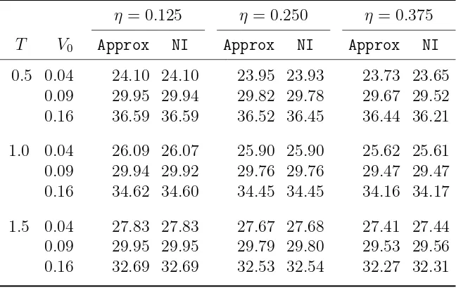
method, and quadgk which uses the adaptive Gauss-Kronrod quadrature method. To the accuracy reported in Table 1, all three routines give identical results. We vary the maturityT, the current instantaneous variance V0, and the volatility coefficient η. The mean-reversion
strength κ is fixed at 2.0, and the long-run variance θ is fixed at 0.09. Feller’s condition requires η < 0.6. Therefore, we consider the three η values in the table. All volatility swap rates reported are in percentage terms. It is interesting to notice that the volatility swap rate in the Heston model with the given parameters is a decreasing function of the volatility coefficientη.13 As we see, the approximation is very accurate in general, and especially when the volatility coefficientη is small or when the maturityT is large.
3.2
European Option Pricing
We now consider the pricing of European-style options under general stochastic volatility models specified in Equations (64) and (65). We consider the special case of ρ = 0. The current approximation technique does not readily generalize itself to nonzeroρ. By the mixing technique in Hull and White (1987), the price of a European call option with strike K and maturityT can be computed as
Cvanilla =
∫ ∞
0
CBS(S0, K, r, δ, T, x) dFξT(x), (75)
whereCBS is the Black-Scholes price given by
CBS(S0, K, r, δ, T, x) =S0e−δTN(d1(x))−Ke−rTN(d2(x)), (76)
with
d1(x) =
log(S0e(r−δ)T/K)
√
x +
√ x
2 , (77)
d2(x) =
log(S0e(r−δ)T/K)
√
x −
√ x
2 . (78)
By integration by parts, we can rewrite Cvanilla as
Cvanilla=
( S0e
−δT
−Ke−rT)++S0e
−δT ∫ ∞
0
(
1−FξT(y
2))n(d
1(y2))dy, (79)
where n(·) is the standard normal probability density function. The above formula is exact and expresses Cvanilla as the sum of two components. The first component is the value of
the option if the price process is deterministic and grows to the forward price. The second component is a strictly positive adjustment due to the fact that the stock process is stochastic.
13
By using the approximation for the cumulative distribution function FξT(·) in the last section, we can approximate the European call option price as
Cvanilla ≈
( S0e
−δT
−Ke−rT)++S0e
−δT ∫ ∞
0
N (
T −µ(y2)
σ(y2)
)
n(d1(y2))dy. (80)
The above approximation works for any Heston-like stochastic volatility model as long as we can compute the functions µ(·) and σ(·). In the case of the Heston model, it offers an alternative to the volatility of volatility expansion in Lewis (2000) and Lipton (2001). It is interesting to notice that the expansion there was developed using complex Fourier inversion while we have worked strictly in the original real space. Also, while it is possible for the price expansion in Lewis (2000) and Lipton (2001) to be negative, the approximate price above is always positive. The integrand is also very well-behaved and decays very fast. A shortcoming is that the current approximation only works for zero correlation.
The complex Fourier inversion is theoretically exact, but its implementation has a number of pitfalls and is far from trivial, especially when maturity is very short or very large, or when the option is far-away from the money. See for example, Carr and Madan (1999), and Kahl and J¨ackel (2005). One advantage of Equation (80) is that it is a very simple integral in the real space. The integrand is bounded in value, and in practice only a limited region needs to be integrated over due to the fact that the integrand decreases exponentially for largey. Our implementation shows that it is extremely fast with a computational time well below one second. Of course, the downside is that it is an approximation, accurate whenη is small.
We use the Heston model to test the accuracy of the approximation for the European call price in Equation (80). The parameters used are: κ = 2.0,θ= 0.09, S0 = 100,r= 0.03, and
δ = 0. We vary the option maturity T, the instantaneous variance V0, the strike price K,
and the volatility coefficient η. The results are reported in Table 2. The exact prices (FI) are computed from numerical Fourier inversion using the known characteristic function for the log stock price under the Heston model. See for example, Lewis (2000). Again, three numerical integration routinesquad,quadl andquadgkin MATLAB are used to cross-verify the numerical integration results. As we see from Table 2, the approximation is very accurate for all parameter combinations of (T, V0, K, η) we have considered.
3.3
Perpetual Timer Forward Pricing
Here we illustrate the usage of the perturbation result obtained in previous section with a perpetual timer forward. This is a contract to exchange one share of the underlying with K
units of cash at a random future date τB at which the daily accumulated realized variance
We use the same general stochastic volatility framework in the last subsection. By risk-neutral pricing, the price Π of the timer forward contract is given by
Π = Π(S0, ξ, V) =E0[e
−rτB
(SτB −K)]. (81)
Notice that because of the perpetual nature, Π does not depend on the calendar timet. In Appendix, we show that we can simplify the above expectation to be the following
Π = Π(S0, ξ, V) =S0Ee0[e−δτ
B]
−KE0[e−rτB]
, (82)
whereEe0 is taken under the measure Qe in which the instantaneous variance process follows
dV =ea(V)dt+ηb(V)dfW . (83)
Here the modified drift function is given by
e
a(V)≡a(V) +ρη√V b(V), (84)
and fW is a Brownian motion under measureQe.
Equation (82) is exact and allows us to use the asymptotic expansion in Proposition 1. This gives the following approximation for Π:
Π≈S0e
−δeµ(B)+1 2δ
2eσ2(B)
−Ke−rµ(B)+12r 2σ2(B)
, (85)
whereµ(B) and σ2(B) are the approximate mean and variance ofτB under measureQ, and
e
µ(B) and eσ2(B) are the approximate mean and variance of τB under measure Qe. All four
quantities can be computed using the method of characteristics illustrated in Appendix. For practical purposes, it is often easier to assume thatea(V) has no explicitη dependence. That is, we absorb the η dependence into other model parameters in ea(V). In many cases, ea(V) turns out to be formally identical to a(V) so no additional effort is needed to compute µe(B) and eσ2(B). This absorbing approach will produce a generalized asymptotic expansion series
instead of the usual power series asymptotic expansion. It gives slightly different formulas for µe(B) and σe2(B), but to second order in η the results are equivalent. Notice that by
Proposition 1, Π given above satisfies the pricing PDE to second order inη:
VΠξ+a(V)ΠV +
1 2η
2b2(V)Π
V V + (r−δ)SΠS+ρη
√
V b(V)ΠSV +
1 2V S
2Π
SS−rΠ =o(η2),
(86)
above, the advantage of Equation (85) is obvious. While a typical implementation of a three-dimensional PDE can take multiple seconds14, the approximation in Equation (85) takes less
than 10−4
seconds given the access of a fast algorithm for the product-log function needed in the Heston model. Fast algorithms for the product-log function are readily available in many software products. For example, in Mathematica, a single evaluation of the product-log functionProductLogtakes about the same time as a cumulative normal distribution function.
From the above approximation, we can approximate the fair delivery priceK∗ as
K∗=S0e
−δµe(B)+1
2δ2σe2(B)erµ(B)− 1
2r2σ2(B)+o(η2). (87)
This is the delivery price that makes the forward contract to have value Π = 0 today.
For the Heston model and the 3/2 model, the computation ofµe(B) andσe2(B) requires no
extra effort once we have computedµ(B) andσ2(B), which are given in Examples 1 and 2 in the last section. This is becauseea(V) takes exactly the same parametric form as a(V) once we absorb theη dependence. For example, in the Heston model, we have
ea(V) =κ(θ−V) +ρηV =eκ(θe−V), (88)
whereκe=κ−ρη,andθe=κθ/eκ.The adjustment for the 3/2 model turns out to be identical. This is not a coincidence since the instantaneous variance process in the 3/2 model is the reciprocal of that in the Heston model. Sinceea(V) is formally identical to a(V) except with different parameters, µe(B) and eσ(B) are also formally identical to µ(B) and σ(B). All we need to do to get µe(B) andeσ(B) is to replaceκ with eκ, andθ with θein Examples 1 and 2. By absorbing a linear η term into ea(V), µe(B) and eσ(B) are now in the form of generalized asymptotic series.
We again carry out a numerical study for the accuracy of the timer forward fair delivery price using the Heston model. For simplicity we assume δ = 0. The reason we choose this special case is that in this case we do not need to solve the three-dimensional PDE in Equation (86). Instead, the exact fair delivery price is computed by numerically solving the PDE that the quantity Υ(ξ, V)≡E0[e−rτB
] satisfies:
VΥξ+a(V)ΥV +
1 2η
2b2(V)Υ
V V −rΥ = 0, (89)
with the boundary condition Υ(B, V) = 1. The fair delivery price is given by
K∗ =
S0
Υ. (90)
14
This is easy to show from Equation (81) since in this zero-dividend caseE0[e−rτB
SτB] =S0. To avoid implementation errors, we employ the standard routine NDSolve in Mathematica, which uses many different methods to numerically solve PDEs, including method of lines, implicit backward differentiation, Runge-Kutta methods, etc. We use a precision goal of 10−8
. Parameters such as step size are automatically chosen by the internal algorithms ofNDSolve. The results are reported in Table 3. We varyr,V0andηas in the table. Other parameters
we use are S0 = 100, κ = 2.0, θ = 0.09, and B = 0.09. For each combination of parameter
values (r, V0, η), we report both the exact fair delivery price (PDE) and the approximated one
(Approx) in Equation (87). As we see in Table 3, the approximation is very accurate for all combinations of parameter values (r, V0, η).
3.4
Perpetual Timer Option Pricing
The perturbation developed in the last section can also be used to price more complicated derivatives. Here we demonstrate this by considering the pricing of perpetual timer call options in the Heston model with ρ = 0. We consider this special case since this is a nice application of the approximation we have developed.15
A perpetual timer call option pays (SτB −K)+ and is only exercisable at time τB, where
B is a contractual variance budget. Timer options have been studied in Bick (1995), Bernard and Cui (2011), Liang, Lemmens, and Tempere (2011), Li (2013), and Li and Mercurio (2013a, 2013b).
By risk-neutral pricing, the price of a timer call is given by
Cperp=E0
[ e−rτB
(SτB −K)+
]
. (91)
By Ito’s lemma, we have
logSt= logS0+ (r−δ)t−
1 2
∫ t
0
Vudu+
∫ t
0
√
VudWuS. (92)
LetFV be the filtration generated by the stochastic processV
u. That is, FV =σ(Vu:u≥0).
Notice τB is measurable in FV. Conditioning on FV, logSτB is normally distributed with mean logS0+ (r−δ)τB−12B and variance B. Integrating out the randomness due toWuS in
Equation (91) then gives
Cperp=E0
[
E0[e−rτB(SτB −K)+| FV
]
=E0[CBS(S0, K, r, δ, τB, B)], (93)
15
whereCBS is the Black-Scholes price defined in Equation (76).
So far the analysis is exact. We can now approximate Cperp by using the approximate
distribution forτB in Proposition 1 to get
Cperp ≈
∫ ∞
−∞
CBS(S0, K, r, δ, u, B) n(u;µ(B), σ2(B)) du. (94)
This integral can be evaluated in closed form to get (see, for example, Appendix of Li, Deng and Zhou (2008) for evaluating the integral)
Cperp≈S0·J(a+, b,−δ, µ(B), σ2(B))−K·J(a−, b,−r, µ(B), σ2(B) )
, (95)
where
a± =
log(S0/K)
√
B ±
√ B
2 , (96)
b= r√−δ
B , (97)
and the functionJis given by
J(a, b, s, m,Σ) =ems+Σs2/2·N (
a+b(m+sΣ)
√
1 +b2Σ
)
. (98)
Interestingly, the timer call price approximation in Equation (95) resembles the Black-Scholes formula for plain-vanilla European-style options. It also has many attractive properties. First, whenr=δ= 0, the formula reduces to known exact result for timer call price. Second, when
η = 0 so that the exercise time is deterministic, the formula reduces to the Black-Scholes formula for plain-vanilla options. Third, the Black-Scholes form makes it easier to compute the Greeks of the timer call option due to the following symmetry:
S0
∂ ∂S0
J(a+, b,−δ, µ(B), σ2(B))=K
∂ ∂S0
J(a−, b,−r, µ(B), σ2(B) )
. (99)
This can be verified by tedious but straightforward calculation. For example, by using the above symmetry, the Delta is given by the following simple expression
∆Cperp ≈J
(
a+, b,−δ, µ(B), σ2(B)). (100)
Notice that the right-hand-side is always positive. Therefore, the approximated timer call price is always positive and strictly increasing inS0, as it should be. Similarly, the Gamma can also
be easily computed and seen to be positive. Finally, we emphasize that our formula is in closed form and therefore extremely fast to evaluate. When implemented in both Mathematica and MATLAB, our program takes less than 10−4
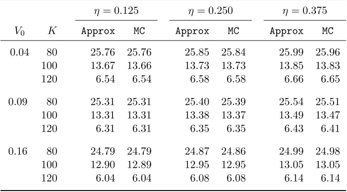
We test the accuracy of the timer call price approximation in Equation (95) using the Heston model. The results are reported in Table 4. The fixed parameters are: r = 0.03,
δ = 0, S0 = 100, κ = 2.0, θ = 0.09, and B = 0.09. We vary the instantaneous variance V0,
the strikeK, and the volatility coefficientη. We use Monte Carlo prices (MC) as benchmarks. The standard errors from Monte Carlo simulations are all in the order of 10−3
or smaller. We use 4 million sample paths with a time step of every two hours. Only the instantaneous variance process needs to be simulated since the Brownian motionWS
u can be integrated out.
See Bernard and Cui (2013) for more details and for a more sophisticated implementation. The integrated variance ξT is used as a control variate for variance reduction, whose mean
is given analytically in the Heston model. Our implementation takes about 30 minutes for each simulation with the desired accuracy goal. As we see, for all parameter combinations (V0, K, η), the approximation is extremely accurate. Unlike some approximation method such
as moment matching, the approximation in Equation (95) is accurate for all values ofK. In fact, when δ= 0, the approximation goes to the correct limit 0 when K goes to infinity, and goes to the correct limit S0 when K goes to 0.
4
Conclusion
Many derivatives products are directly or indirectly associated with integrated diffusion pro-cesses. The hitting time of such an integrated diffusion process plays an very important role in pricing those derivative products. Through perturbation technique, we show that for any diffusion processes, this hitting time is approximately normally distributed when the diffusion coefficient is small. This distributional approximation of the hitting times enables us to reduce many pricing problems to simpler one-dimensional expectations. We illustrate the generality and accuracy of this probabilistic approach using several examples.
The approach has several limitations which we acknowledge here. It cannot handle time-varying drift and diffusion functions right now. It also cannot handle jumps. It also requires that the diffusion coefficient be small which might not be satisfied in some practical applica-tions. Also, although the method in principle works for any drift and diffusion functions, to render it effective in practice we still needs these functions to be simple to obtain closed-form formulas. Also, only Heston model with a limited set of parameters has been tested in this paper. To implement our approximation in product-quality code, extensive testing needs to be carried out beforehand, especially on the greeks.
Appendix
Proof of Proposition 1:
LetX∗
>0 be an arbitrary integration limit. Define two dimensionless variables z0 and z as
follows
z0 =
X−X∗
X∗ , (101)
z= Φ
(
B−ξ+
∫ X
X∗
u a(u)du
)
. (102)
We remark that in a concrete model, it might be easier to just usez0 =X−X∗ without the
scaling or simplyz0 =X. The function Φ is most conveniently chosen to be
Φ(x) = f
−1
(x)−X∗
X∗ , (103)
wheref−1
(x) is the inverse of the function
f(X) =
∫ X
X∗
u
a(u)du. (104)
With this choice of Φ, it is easy to see that z=z0 when ξ =B. This allows us to write the
solution of the ordinary differential equation in simple integral form, as we will see below. The purpose of the above definitions is to change the coordinates from (ξ, V) to the characteristic coordinate (z0, z). Let us express pin terms of the characteristic coordinates z
and z0:
p(ξ, X) =pe(z, z0). (105)
It is easy to check that
Xzξ+a(X)zX = 0. (106)
By utilizing the above equation and chain differential rule, to zeroth-order inη, the PDE for
p(ξ, X) simplifies to an ODE for pe(z, z0) due to cancelation of thepez terms:
e
a(z0)pez0 +λ= 0, (107)
whereea(z0)≡a(X), and with the boundary condition
e
p(z0, z0) = 0. (108)
Therefore, the zeroth-order approximation is given by a simple integral
p0(ξ, X) =ep(z, z0) =
∫ z
z0
λ
Whenη= 0, the processXtis deterministic, and the quantityT0(ξ, X) is just the deterministic
time to exceed the budgetB. Therefore, we haveT0(ξ, X) ≥0 withT0(ξ, X) = 0 if and only
ifξ=B. Notice that the solution ofT0 is given by
T0(ξ, X) =
∫ z
z0
1
e
a(u)du. (110)
To second order in η, the second-order PDE for p(ξ, X) can be approximated by a first-order ODE forpe(z, z0) as follows
e
a(z0)pez0 +λ+
1 2η
2eb2(z
0)[pe0,XX + (pe0,X)2]= 0. (111)
Here eb(z0) ≡ b(X), and pe0,X denotes the partial derivative of p0(ξ, X) with respect to X,
but expressed in terms of the characteristic coordinates z and z0. Similarly for pe0,XX. The
solution ofp(ξ, X) to second order inη is then given by a simple integral
p(ξ, X) =pe(z, z0) =
∫ z
z0
λ+12η2eb2(u)[λTe
0,XX+λ2(Te0,X)2
]
ea(u) du+o(η
2) (112)
≡λ[T0+η2H0] +λ2η2H1+o(η2). (113)
By comparing the last two equalities, the functions H0 and H1 are given by the following
integrals
H0 =
∫ z
z0
eb2(u)Te 0,XX
2ea(u) du, (114)
H1 =
∫ z
z0
eb2(u)(Te 0,X)2
2ea(u) du. (115)
This proves thatE0[eλτB] possesses an asymptotic expansion as follows
E0[eλτB] =eλ[T0+η2H0]+λ2η2H1 +o(η2). (116)
Since by assumptionE0[eλτBτB] andE0[eλτ
B
τB2] are finite for a range of realλvalues containing 0, differentiating the above expansion series once and twice and setting λ = 0 gives the asymptotic expansion series for the first two moments ofτB as follows
E0[τB] =T0+η2H0+o(η2), (117)
E0[(τB)2] = (T0+η2H0)2+ 2η2H1+o(η2). (118)
Therefore, the variance ofτB has the following asymptotic expansion series
Dividing both sides byη2 and taking the limit ofη→0+, we see that H1 ≥0. Furthermore,
H1 = 0 if and only if Var(τB) = 0.
Proof of Equation (82):
This is essentially a change of measure technique. See Li and Mercurio (2013a). However, because random time is involved, it is more elementary to prove the equation from the PDE perspective. To show Equation (82), let
Φ(S, ξ, V) =SΨ(ξ, V)≡E0[e−rτB
SτB
]
. (120)
Notice that Ψ does not depend onS because of the homogeneity of the payoff e−rτB
SτB and the homogeneity of the stock process. By the Feynman-Kac theorem applied using the exit timeτB, Φ(S, ξ, V) satisfies the following PDE
VΦξ+a(V)ΦV +
1 2η
2b2(V)Φ
V V + (r−δ)SΦS+ρη
√
V b(V)ΦSV +
1 2V S
2Φ
SS−rΦ = 0,
(121)
with the boundary condition Φ(S, B, V) = S, and where we use subscripts to denote par-tial derivatives. Since Φ(S, ξ, V) = SΨ(ξ, V), we can easily show that Ψ(ξ, V) satisfies the following PDE
VΨξ+ea(V)ΨV + 1
2η
2b2(V)Ψ
V V −δΨ = 0, (122)
with the boundary condition Ψ(B, V) = 1. A reverse application of the Feynman-Kac theorem using again the exit timeτB now shows that
References
Ahn, D-H., B. Gao. 1999. A parametric nonlinear model of term structure dynamics.Review of Financial Studies12(4), 721–762.
Bernard, C., Z. Cui. 2011. Pricing timer options. Journal of Computational Finance 15(1), 69–104.
Bick, A. 1995. Quadratic-variation-based dynamic strategies.Management Science41(4), 722– 732.
Carr, P., and D.B. Madan. Option valuation using the fast Fourier transform. Journal of Computational Finance2(4), 61–73.
Corless, R.M., G. H. Gonnet, D. E. G. Hare, D. J. Jeffrey, D. E. Knuth. 1996. On the LambertW function.Advances in Computational Mathematics5(1), 329–359.
Cox, J.C., J.E. Ingersoll, and S.A. Ross. 1985. A theory of the term structure of interest rates.
Econometrica53(2), 385–408.
Cui, Z. 2013. Martingale property and pricing for time-homogeneous diffusion models in fi-nance. Ph.D. Dissertation, University of Waterloo.
Dufresne, D. 2001. The integrated square-root process. Working paper, University of Montreal.
Forde, M., and A. Jacquier. 2010. Robust approximations for pricing Asian options and volatil-ity swaps under stochastic volatilvolatil-ity.Applied Mathematical Finance 17(3), 241–259.
Gatheral, J. 2006. The Volatility Surface: A Practitioner’s Guide. John Wiley & Sons.
Gregory, J. 2012. Counterparty Credit Risk and Credit Value Adjustment: A Continuing Challenge for Global Financial Markets. John Wiley & Sons.
Heston, S.L. 1993. A closed-form solution for options with stochastic volatility with applica-tions to bond and currency opapplica-tions.Review of Financial Studies6(2), 327-343.
Hull, J., and A. White. 1987. The pricing of options on assets with stochastic volatilities.
Journal of Finance 42(2), 281–300.
Kahl, C., and P. J¨ackel. 2005. Not-so-complex logarithms in the Heston model. Wilmott Magazine19(9), 94–103.
Karlin, S., and H.M. Taylor. 1991. A Second Course in Stochastic Processes. Academic Press.
Lewis, A.L. 2000. Option Valuation Under Stochastic Volatility. Finance Press, Newport Beach, California.