Liquidity Issues in Indian Sovereign Bond Market

Munich Personal RePEc Archive

Liquidity Issues in Indian Sovereign

Bond Market

Nath, Golaka

CCIL

18 May 2013

Online at

https://mpra.ub.uni-muenchen.de/51633/

Liquidity Issues in Indian Sovereign Bond Market

Golaka C Nath1

Abstract

Liquidity is one of the most important factors after credit risk that affects the bond yields. The

paper uses various measures of liquidity to understand their determinants in Indian sovereign

bond market. The Liquidity measured by parameters like Turnover Ratio and Amihud Illiquidity

Indicator show that these parameters not only have instantaneous relationship with bond yield

but contemporaneous relationship with themselves. Impact Cost is not found to have any

explanatory power. Financial crisis had marginal impact on the Indian sovereign bond market. It

functioned well during the crisis period without much deterioration in general market liquidity

condition as RBI injected large amount of liquidity to the system within a limited time period to

ensure stability in the financial markets in India. However, the notion of flight to safety was

evident as traders started investing largely in Government bonds shunning credit products as the

credit quality in general started to dip. This was duly supported by large issuances of

Government bonds. The study also finds that the electronic order matching system for

government bonds has been successful in improving liquidity and reducing volatility in the

market.

Keywords: liquidity, liquidity premium, bond yield, Indian Sovereign Bonds, Impact Cost, Turnover Ratio, NDS-OM, Liquidity Adjustment Facility

JEL Classification: G12, C58, E43

Liquidity Issues in Indian Sovereign Bond Market

Golaka C Nath2

Liquidity is a major issue in bond markets in emerging countries like India. Corporate bond

markets suffer from higher level of illiquidity vis-à-vis Government bond market in emerging

market economies. Liquidity may have many different things for interpretation. For financial

market, we generally define liquidity as the ease of trading a financial product. If the trading

results in substantial value loss for the asset vis-à-vis its intrinsic value, then we consider the

market for the security as illiquid. If the price loss is marginal or negligible, we consider the

market for the product as liquid. There are many measures of liquidity – volume traded, number

of trades, frequency of trades, bid-ask spread, transaction-by-transaction market impact, etc.

However, finer liquidity estimation using some of these concepts will require high frequency

microstructure data that may not be easily available. Hence, we need to use some simple concept

to measure liquidity over a long period of time.

There are several factors that affect the liquidity – information availability, reliability and quality

of transaction costs, price impact, and search costs, among others. Liquidity affects the asset

prices as investors would require additional compensation to have the inventory of the illiquid

assets which have higher transaction cost vis-à-vis a liquid asset. Amihud and Mendelson (1986,

1989) have demonstrated that lower liquidity in assets resulted in significantly higher average

returns, after controlling for risk and other factors.

The current study examines the liquidity of the Government securities market in India. The

Government securities market is viewed as one of the most important financial market as it links

economic activity to interest rate. Central banks use the market to perform domestic monetary

operations like infusing liquidity to the system or absorbing excess liquidity in the system

through Repo windows or Open Market Operations (OMO). They use the market to extract

information on forward interest rates and inflation expectations. The market also provides

benchmarks to the traders to use it for corporate credit. Liquidity of this market is important to

all stake holders. The market liquidity has an impact on a central bank’s policy making

specifically when the central bank has additional responsibility of ensuring the smooth

borrowing programme for the Government. There are three distinct channels through which we

can study this impact. (a) Liquidity has an impact on monetary policy formulation of the central

bank as the decision to follow a tight or easy monetary policy depends on the available liquidity

in the system. Financial asset price information (Bond prices) provide valuable clue not only on

current market condition, they also provide vital information on future monetary conditions and

hence this can be used in the formulation and implementation of monetary policy by the central

bank. Market liquidity affects price of assets as illiquid securities add significant cost of holding

an asset inventory to its price. As liquidity has cost, its gets built into the price. Liquidity

condition in the market also affects the transmission of monetary policy actions. Central Banks

conduct OMO to easy liquidity condition in the market so that the interest rate is moderated to

targeted levels. Market liquidity has a more direct impact on monetary policy implementation.

(b) Market liquidity may at times cause systemic disruption and put pressure on Governments

and central banks to act. Financial crisis of 2007-09 was accentuated more due to tight market

liquidity as funds dried up in the market and many firms had to face liquidation as they did not

have sufficient liquidity options to survive the tight condition. Depending on the level of market

liquidity, at times, liquidity issues give rise to solvency problems at key financial intermediaries.

The liquidity problems can lead to systemic failure in payment systems (liquidity risk) and lead

to the collapse in credit allocation. During recent financial crisis, most of the central banks

around the world worked overtime to inject liquidity to the financial system through banking and

near-banking channels to avoid systemic payment collapse. Hence, insufficient market liquidity

will have resultant impact on a central bank’s activities both as a lender of last resort and in its

supervision of financial stability. An inadequate liquidity situation may lead to inaccurate

estimation of market risk and may create disruption in the market discipline posing serious

challenge to the central bank’s ability to supervise through prudential regulation. (c) In the aftermath of financial crisis, it was observed that most of the Governments around the world

have very high level of outstanding debt because of their support to the financial system during

Governments. A central bank would always work in close coordination with the Government to

enhance the integrity and efficiency of the Government securities market. Central banks around

the world released funds to the monetary system by following easy monetary policy regimes so

that transmission effect results in smooth credit and market risk environment and to obviate

bankruptcy issues. Most of the central banks used bond buying programmes to pump liquidity to

support the market.

A market is liquid if traders can execute their trades immediately, and where large deals have

little impact on current and subsequent prices or bid-ask spreads. The market liquidity is better

explained over four dimensions: immediacy, depth, width (bid-ask spread), and resiliency. All

these dimensions of liquidity interact with each other and makes market liquidity a complex

issue. A market is generally considered to be liquid if it is possible for a trader to sell or buy

large amounts of securities in a minimum number of transactions with little impact on prices.

Gravelle (1999a) explained liquidity according to four dimensions: (a) immediacy, or the speed

of doing a transaction; (b) depth, which refers to the maximum amount of a security which can

be traded at a given price; (c) width, or the bid-ask spread3, which is the cost of accessing

liquidity indicating a wider spread means lower liquidity; and (d) resiliency, which captures how

fast prices revert to their equilibrium after a transaction.

Price impact explains the depth of the market. In a liquid market, large quantities of securities

can be traded without affecting the price. But in many markets – specifically in emerging

markets, it might be difficult to find a counterparty who is willing to buy or sell a specific

security and the holder of the bond need to provide higher capital to maintain the inventory. The

liquidity of a specific bond may affect the price. If the investor wants an immediate execution of

a sell order, he will have either to sell at a discount, or take the risk of waiting to realize the

price. Liquidity is an important determinant of bond yield and returns. The liquidity component

of bonds can explain a larger fraction of the yield than the default component itself. The size and

the turnover volume of the secondary market affect the liquidity of the bonds. If a market has

sufficient buyers and sellers to facilitate trading of a bond, its ability to respond to market events

is higher. Illiquid bonds respond less quickly to market events due to low depth and hence they

3 _{Bid-Ask spread is the difference between Best Buy Price and Best Sell Price. The spread is the compensation}

are more likely to see wide swings in prices. The traders will penalize higher volatility and

demand high yield which will be reflected in the bond’s price.

Liquidity in the bond market can be enhanced in a market with improvement in market’s

institutional structures by introduction of electronic dealing platforms, improving the depth of

the market by bringing in new participants like Primary Dealers along with market making

mechanism, improved disclosure standards, tax factors including withholding taxes, increasing

floating stocks in the market, providing hedging instruments for risk management like

derivatives, well-functioning clearing and settlement systems, introduction of STRIPS Program

for government securities, Open Market Operations by the Central Bank, structured buyback

programmes, regular re-opening of issues to ensure availability of comfortable level of floating

stocks, etc. Size indicators like transaction volumes cannot be used as reliable liquidity measure

as it does not capture any age-induced declines in liquidity. In many markets, introduction of

electronic platforms have provided ease in trading and have helped in reducing cost of trading. In

India, the experiment with the NDS-OM4 trading system for Government bonds has paid rich

dividend for all stake holders. However, market participants still preferred using conventional

trading channel for off-the-run bonds and other sovereign securities like T-bills and State

Development Loans5 (SDL) even though NDS-OM provides better electronic order book

options. In most countries, liquid secondary markets are based on the following cornerstones: (i)

higher incidence of issuance in critical tenors like benchmark points; (ii) well-functioning repo

and short sell markets; (iii) well-functioning derivatives (both OTC and exchange traded)

markets to hedge risks; (iv) facilitating price discovery mechanism; and (v) supporting a network

of primary dealers.

The concept of liquidity is complex, although empirically, a single dimension such the ability to

trade a security with minimal impact on its price is considered while measuring liquidity in

quantitative terms. The liquidity in Indian Government bond market could be enhanced to some

extent in recent years by using the key building-blocks like: (i) sound institutions and macro

4 _{Negotiated Dealing Platform – Order Matching (NDS-OM) system is owned by Reserve Bank of India and}

facilitates secondary market deals in Government Securities including T-Bills and State Development Loans (SDL) among banks and Institutions sans intermediaries.

5 _{Federal States in India issue securities to fund the deficit of the respective States at market determined rates}

policies; (ii) an efficient and robust infrastructure; (iii) a well-functioning repo market; (iv)

adequate information flows; and (v) a diversified investor base including facilitating foreign

investment in Government bonds.

Indian Treasury bond market has gone through major changes during last one decade or so.

Introduction of primary dealer system, well-structured auction mechanism with auction calendar,

structured clearing and settlement mechanism with CCP6 provisions, availability of OTC Rupee

derivatives products, anonymous trading platform like NDS-OM providing efficient price

discovery, well developed repo and repo-variant market7, provisions of short selling, etc. have

been instrumental in improving the market microstructure in Indian Government bond market.

The Government bond market is a unique experiment with enabling provisions for execution of

trades using brokers, directly talking to a counter party over telephone and online anonymous

order matching mechanism.

The present paper makes an attempt to understand the issues related to liquidity behavior of

Indian Government securities market as well as tries to find out how various indicators of

liquidity is used in the market. It also tries to understand how realistically the liquidity indicators

are used in the market and what factors are considered as determinants of the liquidity indicators.

The paper is arranged into following – Section 1 deals with Indian market microstructure;

Section 2 discusses some stylized facts; Section 3 deals in liquidity measurement and

determinants; Section 4 deals with volatilities and Section 5 gives concluding remarks.

Indian Market Microstructure

Indian bond market is dominated by Government securities – in both primary and secondary

markets. Government bond market includes the securities issued not only by the Government of

India8 but also the securities issued by various federal States. The primary market auctions for

6 _{Central Counter Party (CCP) – providing guarantee of settlement of the trades executed by the traders.}

7 _{Collateralized Borrowing and Lending Obligations (CBLO) is a tradable repo but the security is held with third}

party (held-in-custody).

both Government securities and Treasury Bills are conducted through electronic auction system

and the said system also facilitates “When Issued Market”.

Table – 1: Snapshot of the Indian Government Securities Market

M9_{2009 M2010 M2011 M2012 M2013}

No. of Outstanding stock 132 128 122 121 118

Outstanding stock (` In billion) 17,061 20,335 23,500 27,830 32,445

Outstanding stock as ratio of GDP (%)* 38.63 42.44 44.37 49.42 56.28

Turnover/GDP (%)* 468.66 628.68 418.02 391.23 629.64

Average maturity of the securities issued during the year (Years) 13.82 11.17 11.63 12.67 13.60

Weighted average cost of the securities issued during the year (%) 7.69 7.23 7.91 8.52 8.36

Minimum and maximum maturities of stock issued during the year (Years) 4 - 30 2 - 30 2 - 30 5 - 30 4 - 30

PD's share in the Outright turnover - Secondary Market 18.77 15.84 18.98 26.35 17.22

Transactions on CCIL (Face value ` In billion)# 62,545 89,867 69,702 72,521 119,948

Turnover Ratio (%) 0.9606 0.6188 0.6450 0.6641 1.7881

10-Year Yield (%)@ 7.01 7.79 7.98 8.53 7.96

Outstanding Treasury Bills (` In billion) 1,503 1,375 1,413 2,670 2,998

Issuances of Cash Management Bills (` In billion) - - 120 930 -

91 Day T-bill cut-off Yield (%)$ 4.95 4.38 7.31 9.02 8.19

Notes: * - GDP at market price (at 2004-05 prices). Q4 of 2012-13 is the approximation of Q3 with 5% p.a. GDP growth.

# - Transaction on CCIL comprises of total outright and repo value settled.

@ - Last trading day of the financial year.

$ - Last Auction of the financial year. Turnover ratio is daily average trades volume divided by Face Value outstanding for Gilts Source: CCIL

During last few years, Government of India has been steadily increasing its market borrowing

and funds almost 90% of its fiscal deficit through such market borrowings. In FY2011-12, large

amount were raised by issuing T-bills of various durations. During FY2011-11 and FY2011-12,

some Cash Management Bills10 were also issued to raise funds from the system. As these large

borrowings have put pressure in the market liquidity, RBI has to resort to Open Market

Operations (OMO) on various occasions to infuse liquidity to the system. This liquidity infusion

is in addition to the daily LAF Repo conducted by RBI to moderate money supply in the system.

9 _{March is the typical Financial Year End (FY 2011-12 mean Year ended March 2012).}

Table -2: Government Borrowing Details (` Crore11₎

FY G-Sec SDL T-Bill

Gross Net Gross Net Gross Net

2007-08 194050 146112 67779 56224 314496 -33155

2008-09 277000 219302 118138 103766 360912 31827

2009-10 428306 327369 131122 114883 385875 -13274

2010-11 437000 322677 104039 88398 343765 327

2011-12 510000 426025 158632 136643 630813 132193

2012-13 558000 467384 177279 146657 802830 32743

Source: CCIL

The high borrowing level has to be managed by the Reserve Bank of India (RBI) through

uniform price based auctions as well as through infusion of liquidity to the system. The liquidity

shortage has been continuing for a long time in India (since July’10) and this has resulted in RBI

injecting good amount of liquidity to the system using daily LAF. On many occasions, OMOs

have to be conducted just before the auctions for Government securities. This has helped to

ensure smooth sailing of auctions as well as helping to moderate yield.

Unlike US and other developed markets, Government bond market in India is a wholesale

market with very little or negligible participation from retail investors. The secondary market

microstructure underwent dramatic change after introduction of NDS-OM system which

facilitated anonymous trading in Government bonds like equities with an efficient price

discovery mechanism but without any intermediary. Brokers or intermediaries which facilitated

about 80% of the trading before introduction of NDS-OM system in Aug 2005 did not have

access to the new system as the new system was owned by Reserve Bank of India and directly

allows traders to trade accessing large market provided they have Constituent Gilts Accounts12.

The web-based application within NDS-OM system allows direct market access to constituents

to trade in the wholesale institutional market with efficient price discovery. The participants had

three options to choose: (a) directly negotiating with each other for a deal; (b) taking the help of

a broker to identify the counter party to trade a security; (c) directly becoming a member of the

11 _{1 crore is equivalent to 10 million.}

12 _{An electronic demat account maintained by an investor with a service provider like a bank to hold the balances}

new order driven system which was STP13 enabled from the start. However, the new system captured about 60% of the market immediately after its introduction. The market share of the

new trading system is steady at about 80%. Broking companies have very little role with about

8% market share.

The new trading system, NDS-OM, provided higher liquidity to the system with an active order

book management system and efficiency in price discovery. The traders could see the depth of

the market anytime with buy and sell orders coming to the system with time stamp. Proprietary

deals by Banks and Institutions accounted for about 87% in terms of value (90% in terms of

number of deals). Participation in trading was also linked to a bank’s total holding of

Government securities. Typically a major part of a bank’s holding of Government securities is in

Held to Maturity (HTM) category as banks are allowed to put a part of the security (currently

upto 23% of the Net Demand and Term Liabilities (NDTL) which is exactly equal to the

Statutory Liquidity Ratio (SLR)) in the said category which does not envisage any provision for

mark-to-market losses as it is expected to be held till its redemption. The remaining part of the

securities holding balance can be held in Available for Sale or Held for Trading which will

require regular provisioning and mark-to-market.

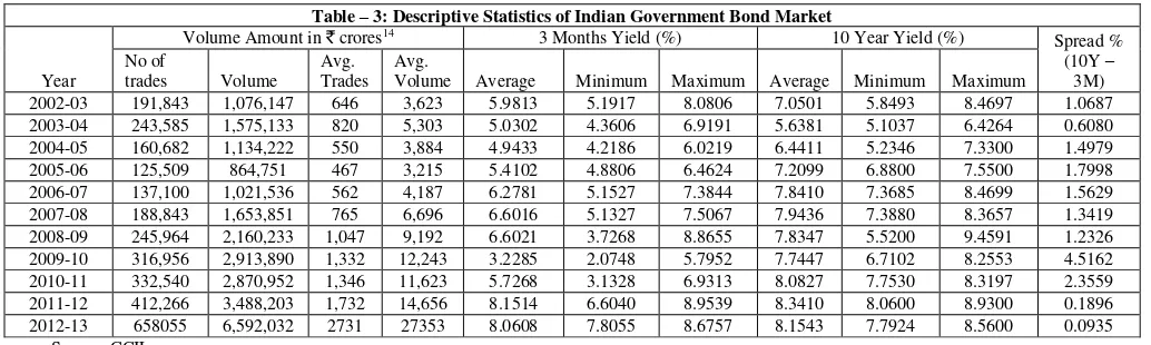
Table – 3: Descriptive Statistics of Indian Government Bond Market

Year

Volume Amount in ` crores14 _{3 Months Yield (%) 10 Year Yield (%)}

Spread % (10Y –

3M) No of

trades Volume Avg. Trades

Avg.

Volume Average Minimum Maximum Average Minimum Maximum

2002-03 191,843 1,076,147 646 3,623 5.9813 5.1917 8.0806 7.0501 5.8493 8.4697 1.0687 2003-04 243,585 1,575,133 820 5,303 5.0302 4.3606 6.9191 5.6381 5.1037 6.4264 0.6080 2004-05 160,682 1,134,222 550 3,884 4.9433 4.2186 6.0219 6.4411 5.2346 7.3300 1.4979 2005-06 125,509 864,751 467 3,215 5.4102 4.8806 6.4624 7.2099 6.8800 7.5500 1.7998 2006-07 137,100 1,021,536 562 4,187 6.2781 5.1527 7.3844 7.8410 7.3685 8.4699 1.5629 2007-08 188,843 1,653,851 765 6,696 6.6016 5.1327 7.5067 7.9436 7.3880 8.3657 1.3419 2008-09 245,964 2,160,233 1,047 9,192 6.6021 3.7268 8.8655 7.8347 5.5200 9.4591 1.2326 2009-10 316,956 2,913,890 1,332 12,243 3.2285 2.0748 5.7952 7.7447 6.7102 8.2553 4.5162 2010-11 332,540 2,870,952 1,346 11,623 5.7268 3.1328 6.9313 8.0827 7.7530 8.3197 2.3559 2011-12 412,266 3,488,203 1,732 14,656 8.1514 6.6040 8.9539 8.3410 8.0600 8.9300 0.1896 2012-13 658055 6,592,032 2731 27353 8.0608 7.8055 8.6757 8.1543 7.7924 8.5600 0.0935

Source: CCIL

Banks alone account for about 72%15 of total trading in Government securities while Primary

Dealers account for about 17% of trading and other Institutions like Mutual Funds and Insurance

13 _{Straight Through Processing (STP) – a process through which a trade executed in the NDS-OM system will}

directly go for multilateral netting through the clearing house and final settlement in central bank money. Other deals have to be reported to RBI within a certain prescribed time after execution. Broker driven deals have to be reported by selling Bank to the RBI and Broker has also to report the same deal to the Stock Exchange.

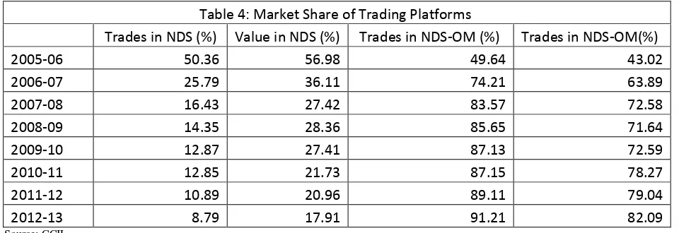
companies account for about 9% of trading. Indian Government bond market is divided into two

distinct systems – (i) an anonymous order driven system (NDS-OM) introduced in Aug 2005 and

(ii) a trade reporting system where trades are executed over phone by market participants and

then reported to the central server managed by Reserve Bank of India (RBI) within a particular

time frame (30 minutes)16. Market participants, mainly institutions, are free to choose any of the

above two systems for their deals in Government securities and T-bills. The NDS-OM system

contributes a significant part of the market transactions in number of deals as well in terms of

value of deals and has established itself as the most preferred platform for executing trades.

Table 4: Market Share of Trading Platforms

Trades in NDS (%) Value in NDS (%) Trades in NDS-OM (%) Trades in NDS-OM(%)

2005-06 50.36 56.98 49.64 43.02

2006-07 25.79 36.11 74.21 63.89

2007-08 16.43 27.42 83.57 72.58

2008-09 14.35 28.36 85.65 71.64

2009-10 12.87 27.41 87.13 72.59

2010-11 12.85 21.73 87.15 78.27

2011-12 10.89 20.96 89.11 79.04

2012-13 8.79 17.91 91.21 82.09

Source: CCIL

Some Stylized Facts Liquidity Infusion

Liquidity in the market depends on many factors. The most important issue in liquidity is the

support from the central bank to the banking system to access liquidity from the monetary

system. RBI uses daily Liquidity Adjustment Facility (LAF) to moderate money supply in the

system – if the banking system has excess liquidity, it can be parked at the central bank with a

fixed return using policy reverse repo rate through LAF and if the banking system faces shortage

of liquidity, RBI injects liquidity to the system using a fixed policy repo rate through LAF. In

case the bank is not able to cover its position and still faces shortage, RBI supports the bank with

a Marginal Standing Facility using a special LAF window at the end of the business day. The net

LAF indicates the liquidity condition in the market. During financial crisis period, we find that

liquidity shortage in the market resulted in RBI injecting funds to the system in mid-2008 and in

15 _{As of Dec’12 statistics.}

Sep-Oct’08, the shortage was more than 1% of the NDTL. Further, in order to fight the effect of the financial crisis, RBI reduced the policy Repo Rate on multiple occasions, reduced CRR and

SLR and infused liquidity in the system. This substantial injection of liquidity resulted in excess

funds with the banking system as credit delivery started sinking due to the crisis. Banks started

parking these excess funds with RBI at policy reverse repo rate. The liquidity infusion helped the

market to increase their participation in bond market as interest rate started dipping due to

infusion of huge liquidity to the system coupled with reduction in policy rates and drop in credit

delivery.

Table 5: Actual/Potential Release of Primary Liquidity (since mid-September 2008 (till Mar 2009))

Measure/Facility Amount (`. Crore)

Monetary Policy Operations (1 to 3)

1. Cash Reserve Ratio (CRR) Reduction 1,60,000

2.Open Market Operations 68,835

3. MSS Unwinding/De-sequestering 97,781

Extension of Liquidity Facilities (4 to 8)

4. Term Repo Facility 60,000

5. Increase in Export Credit Refinance 25,512

6. Special Refinance Facility for SCBs (Non-RRB) 38,500

7. Refinance Facility for SIDBI/NHB/EXIM Bank 16,000

8. Liquidity Facility for NBFCs through SPV 25,000

Total (1 to 8) 4,91,628

Memo:

Statutory Liquidity Ratio (SLR) Reduction 40,000

Source: RBI

The liquidity infusion also helps banking system to invest in bonds thereby increasing the bond

turnover in the market. Since mid-2010, Indian market is going through a tight liquidity

condition for which RBI has been injecting liquidity through LAF repo window and occasional

OMO. The proactive policy initiatives were taken by RBI to avoid contraction of the RBI

balance sheet and the same aimed at ensuring non-inflationary growth of money supply in the

Table 6: LAF Support as a percentage of NDTL

Year 2005 2006 2007 2008 2009 2010 2011 2012 2013

LAF 0.92% 0.90% 0.10% -0.11% 2.23% -0.13% -1.12% -1.44% -1.49%

TR17 0.53 0.63 0.70 1.05 1.22 0.97 0.84 1.30 2.34

Source: CCIL, RBI

Trading Activity

Though there are large numbers of securities (there are 110 securities including special securities

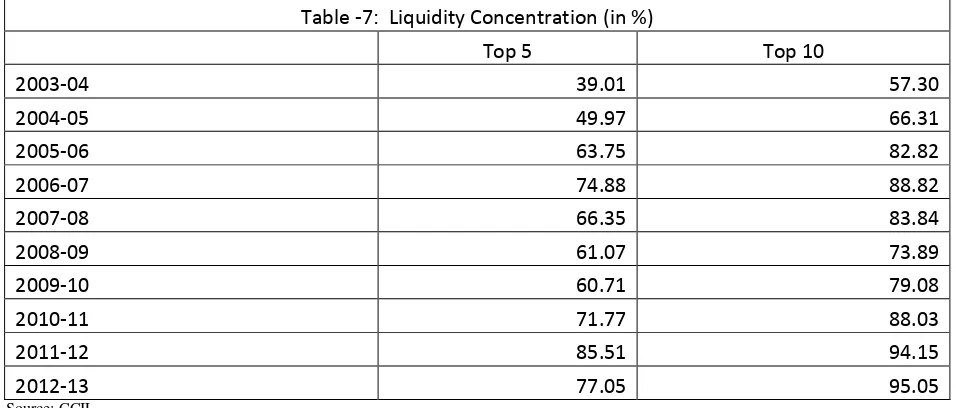
but excluding floating rate bonds as on March’13) extending maturity upto 30 years issued by the Government and available for trading in the market, trading is concentrated on few securities.

Indian Government bond market faces high concentration in benchmark securities like 10-year

and 5-year maturities. Though there are large number of securities issued by the Government,

trading in 10 securities constitute about 95% of the trading in terms of value. Hence most of the

securities are relatively illiquid. Trading level in the market is also sensitive to the net LAF level.

The correlation between Net LAF and Trading volume is -0.39. There is liquidity concentration

in few securities like 10-year benchmark. The concentration of liquidity in few securities has

increased in recent years.

Table -7: Liquidity Concentration (in %)

Top 5 Top 10

2003-04 39.01 57.30

2004-05 49.97 66.31

2005-06 63.75 82.82

2006-07 74.88 88.82

2007-08 66.35 83.84

2008-09 61.07 73.89

2009-10 60.71 79.08

2010-11 71.77 88.03

2011-12 85.51 94.15

2012-13 77.05 95.05

Source: CCIL

17 _{Turnover Ratio (TR) is the average daily trading in Government securities as a proportion to the outstanding Face}

Trading concentration in benchmark securities has been hallmark of the Indian Government

securities market. After the financial crisis, market interest in long term bonds have come down

significantly.

Table – 8: Maturity Bucket Trading Distribution

Category M2003 M2004 M2005 M2006 M2007 M2008 M2009 M2010 M2011 M2012 M2013 Current

upto 5 Years 7.08 9.07 23.64 26.44 27.68 22.81 19.46 27.15 19.57 3.49 6.81 15.29

5 to 10 Years 54.42 36.75 45.05 29.10 58.61 53.08 54.43 59.07 39.68 75.19 41.22 34.95

10 to 20 Years 35.54 52.53 29.35 39.78 4.62 8.88 13.69 11.58 39.20 20.34 49.81 48.53

20 to 30 Years 2.96 1.65 1.95 4.68 9.09 15.24 12.41 2.21 1.55 0.98 2.16 1.22

Source: CCIL

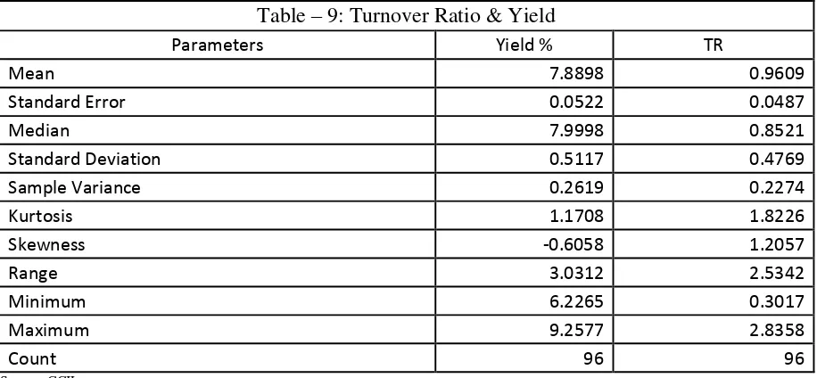
Liquidity Measurement and Determinants Turnover Ratio

Bond Market liquidity can be measured by Bonds Turnover Ratio (TR). The ratio shows the

extent of daily trading volume in the secondary market (buy and sell) relative to the amount of

bonds outstanding measured in terms of Face Value. This ratio is computed for securities using

only outright purchases / sales andexcludes repo / repurchases transactions. A secondary market

is said to be active when the TR is high.

Table – 9: Turnover Ratio & Yield

Parameters Yield % TR

Mean 7.8898 0.9609

Standard Error 0.0522 0.0487

Median 7.9998 0.8521

Standard Deviation 0.5117 0.4769

Sample Variance 0.2619 0.2274

Kurtosis 1.1708 1.8226

Skewness -0.6058 1.2057

Range 3.0312 2.5342

Minimum 6.2265 0.3017

Maximum 9.2577 2.8358

Count 96 96

Source: CCIL

TR can be used as a relative measure to understand liquidity. The same widely varies among

securities. For some of the on-the-run treasuries, the TR is very high as concentration of trading

typically held in the books of the banks under “Held Till Maturity” category investment. Typically TR will be high when market liquidity is high. High market liquidity indicates lower

interest rate scenario prevailing at that point in time (in relative term). TR is a very important and

useful proxy for liquidity in the market. When interest rate level is lower, it encourages traders to

build positions. At higher interest rate, traders do not want to keep high inventory of stocks and

hence trading volumes takes a dip.

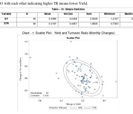
In India, TR and 10 year yield (monthly changes) are observed to have a negative correlation of

0.43 with each other indicating higher TR means lower Yield.

Table – 10: Simple Statistics

Variable N Mean Std Dev Sum Minimum Maximum

DY 94 0.0069 0.2458 0.6505 -1.2167 0.7714

DTR 94 0.0197 0.4067 1.8500 -0.7500 1.51

Chart - 1: Scatter Plot - Yield and Turnover Ratio (Monthly Changes)

Table –11: Pearson Correlation Statistics (Fisher's z Transformation) Variable With

Variable

N Sample

Correlation

Fisher's z Bias Adjustment

Correlation Estimate

95% Confidence Limits

p Value for

H0:Rho=0

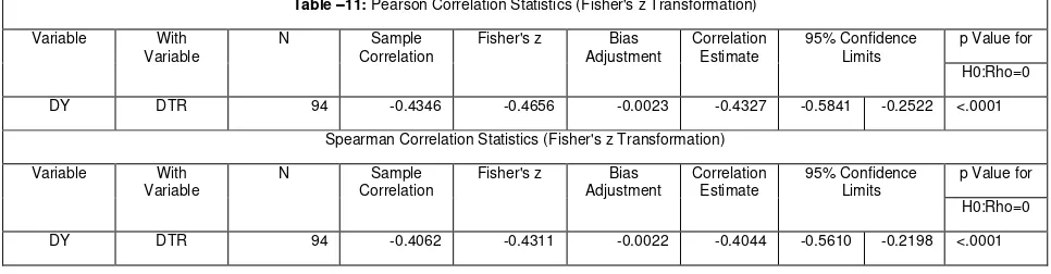
DY DTR 94 -0.4346 -0.4656 -0.0023 -0.4327 -0.5841 -0.2522 <.0001

Spearman Correlation Statistics (Fisher's z Transformation)

Variable With Variable

N Sample

Correlation

Fisher's z Bias Adjustment

Correlation Estimate

95% Confidence Limits

p Value for

H0:Rho=0

DY DTR 94 -0.4062 -0.4311 -0.0022 -0.4044 -0.5610 -0.2198 <.0001

Graphically they follow a close trend. During financial crisis, there was substantial drop in TR.

In order to understand the true relation between TR and Yield, we fitted a simple model using the

TR and Yield (monthly changes). The regression R-sq was 0.19. The linearly fitted model

showed that Yield and TR have statistically significant relationship. We re-specified the model

with inclusion of the lagged yields as additional variables and found that the R-sq improved to

0.38.

Table – 9: Parameter Estimates

Variable DF Estimate Standard t Value Approx

Error Pr > |t|

Intercept 1 0.0198 0.0343 0.58 0.5658

DY 1 -1.0121* 0.1536 -6.59 <.0001

Lag 1 DY 1 0.789* 0.1639 4.81 <.0001

Lag 2 DY 1 -0.0158 0.1534 -0.1 0.918

R-Sq – 0.38, DW – 2.61 RMSE – 0.3282, * - significant at 1%

Since most of the time series data has an autoregressive structure, we re-specified the regression

model with inclusion of lagged variables of the TR in the equation upto 5 lags18 _{along with the}

yields and lagged yields.

𝑇𝑅𝑡= 𝛼 + 𝛽1∗ 𝐷𝑌1 + 𝛽2∗ 𝐷𝑌2 + 𝛾1∗ 𝐿𝑇𝑅1 + 𝛾2∗ 𝐿𝑇𝑅2 + 𝛾3∗ 𝐿𝑇𝑅3 + 𝛾4∗ 𝐿𝑇𝑅4 + 𝛾5∗ 𝐿𝑇𝑅5 + 𝜀𝑡

Table – 10: Parameter Estimates

Variable DF Estimate Standard t Value Approx

Error Pr > |t|

Intercept 1 0.0475 0.032 1.48 0.1420

DY 1 -1.0343* 0.1449 -7.14 <.0001

LY 1 0.2002 0.1879 1.07 0.2900

LTR1 1 -0.5218* 0.1105 -4.72 <.0001

LTR2 1 -0.4858* 0.122 -3.98 0.0001

LTR3 1 -0.2797** 0.1154 -2.42 0.0176

LTR4 1 -0.2267 0.1018 -2.23 0.0287

LTR5 1 -0.0554 0.0983 -0.56 0.5749

R-Sq – 0.53, DW – 1.9919 _RMSE – _{0.2965 * - significant at 1% and ** - significant at 5%}

The estimated equation shows that TR has a long memory and it gets influenced by lagged

values of TR upto 4 months though lag 3 and 4 are week and statistically significant only at 5%

level. It also showed that lagged yield is not statistically significant. We re-estimated the model

with these lagged variables (OLS). The signs of the estimated equation show clearly that change

in liquidity measured by TR is negatively related to the level of Yield and positively to previous

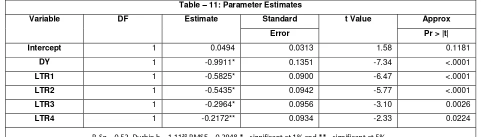
months’ TR. We also tried to re-estimate the model with an autoregressive process using only 4

lagged values of TR and DY.

Table – 11: Parameter Estimates

Variable DF Estimate Standard t Value Approx

Error Pr > |t|

Intercept 1 0.0494 0.0313 1.58 0.1181

DY 1 -0.9911* 0.1351 -7.34 <.0001

LTR1 1 -0.5825* 0.0900 -6.47 <.0001

LTR2 1 -0.5435* 0.0942 -5.77 <.0001

LTR3 1 -0.2964* 0.0956 -3.10 0.0026

LTR4 1 -0.2172** 0.0934 -2.33 0.0224

R-Sq – 0.52, Durbin h – 1.1120 _{RMSE – 0.2948 * - significant at 1% and ** - significant at 5%}

The total R-Sq statistic computed from the above autoregressive model is 0.52. The Regression

R-Sq was the R-Sq statistic for a regression of transformed variables adjusted for the estimated

autocorrelation. The parameter estimates gives the Maximum Likelihood (ML) estimates of the

19 _{Since lagged values are included in the equation, DW stat is not strictly valid.}

20 _{Since lagged values are included in the equation, DW stat is not strictly valid. Durbin h is used to test for}

regression coefficients. The fitted model shows that turnover ratio has contemporaneous

relationship with its own lagged information but has an instantaneous relationship with the yield.

Amihud Illiquidity Indicator

Amihud (2002) measured illiquidity of the stock using a measure called ILLIQ which is the daily

ratio of absolute price change to its value traded. This is interpreted as the daily price response

linked to trading value. This ratio works as a good measure for estimating price impact. There

are other measures of liquidity but some of such measures will require high frequency

microstructure data (e.g. for calculating bid-ask spread). The measure proposed by Amihud can

be easily constructed with usual available data of daily prices for a longer period to test the

effects over time of illiquidity on ex-ante and contemporaneous bond returns. This illiquidity

measure can be linked with other simple measures of illiquidity. Amihud found that both across

stocks and over time (for NYSE during 1964-1997), expected returns are an increasing function

of expected liquidity. He found that ILLIQ has a positive and highly significant effect on

expected returns. He found that higher realized illiquidity raises expected illiquidity that in turn

raises expected returns.

Following Amihud, bond illiquidity is defined in this paper as the ratio of daily absolute return to

the trading value on that day. Daily absolute return is calculated by taking the difference between

closing price and opening price of the bonds. Since there are two distinct platforms for doing

and/or recording a transaction in India, NDS-OM platform dominates with large market share.

Though same security can be traded either in OTC market and gets reported in NDS system or it

can be anonymously traded in NDS-OM system, it is necessary to adjust the scale factor (trading

multiple) in ILLIQ ratio computed for NDS system vis-à-vis NDS-OM system. Since NDS-OM

market is visible to all traders in the market on almost real time basis, deals in OTC market may

be executed by dealers after comparing the price/yield in NDS-OM system. In order to have

better understanding of the liquidity dynamics in Indian Government securities market, we

divided the securities into three categories in terms of their number of deals in a day. If the

number of deals exceeds 15 in a day, it is considered as “Liquid”, if the number of deals exceeds

High and Low prices are same – all deals are considered as “special” and might have taken place at the same price. These deals may be the ones which are executed by the same dealers (at least

in one side of the deal) and hence executed at a single price. We constituted our dataset with

securities that have at least 3 trades in a day and dropped all non-market lot deals (below

50million). However, the Amihud ILLIQ ratio that was computed for NDS are scaled (adjusted)

using the trading value ratio (the ratio of value of deals in NDS-OM and NDS). This scaling is

absolutely necessary to make them comparable in terms of their liquidity parameters. After

scaling the ILLIQ ratio, both NDS and NDS-OM became comparable for analysis. It is observed

that the scaling factor is less than 1 for semi-liquid and illiquid securities while for liquid

securities, the scaling factor is greater than one and very high. The Amihud ratio has been

multiplied by 10^7 for reporting results.

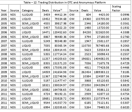
Table – 12: Trading Distribution in OTC and Anonymous Platform

Year Source Category Deals Value21 _{Source Deals Value}

Scaling Factor

2005 NDS ILLIQUID 3459 44412.34 OM 604 4425.00 0.0996

2005 NDS LIQUID 13452 79334.68 OM 24360 133705.00 1.6853

2005 NDS SEMI_LIQUID 4555 39817.98 OM 2346 14180.00 0.3561

2006 NDS ILLIQUID 5457 71022.23 OM 1480 13720.00 0.1932

2006 NDS LIQUID 14471 120452.60 OM 84230 522620.00 4.3388

2006 NDS SEMI_LIQUID 8867 98480.36 OM 3794 27180.00 0.2760

2007 NDS ILLIQUID 5249 90348.80 OM 1947 25811.07 0.2857

2007 NDS LIQUID 7035 83365.54 OM 110730 767485.68 9.2063

2007 NDS SEMI_LIQUID 8458 130414.45 OM 5623 53554.54 0.4106

2008 NDS ILLIQUID 5355 117714.34 OM 2523 30098.43 0.2557

2008 NDS LIQUID 11257 143203.63 OM 196821 1404082.05 9.8048

2008 NDS SEMI_LIQUID 8355 151571.20 OM 7036 71675.78 0.4729

2009 NDS ILLIQUID 6905 173391.08 OM 4811 77428.08 0.4466

2009 NDS LIQUID 14059 241654.98 OM 262454 1889383.22 7.8185

2009 NDS SEMI_LIQUID 11367 222748.96 OM 10384 124597.36 0.5594

2010 NDS ILLIQUID 5197 111477.47 OM 3868 65120.65 0.5842

2010 NDS LIQUID 18321 230024.97 OM 272050 2043296.97 8.8829

2010 NDS SEMI_LIQUID 10082 164706.65 OM 7182 95861.22 0.5820

2011 NDS ILLIQUID 4724 90192.21 OM 2939 42877.10 0.4754

2011 NDS LIQUID 18681 253828.72 OM 300355 2137379.45 8.4206

2011 NDS SEMI_LIQUID 9544 141557.70 OM 6185 75121.81 0.5307

2012 NDS ILLIQUID 6994 132035.65 OM 5264 79485.50 0.6020

2012 NDS LIQUID 25284 542747.61 OM 483858 3917165.57 7.2173

2012 NDS SEMI_LIQUID 12573 180700.67 OM 11721 145392.90 0.8046

2013 NDS ILLIQUID 515 7586.96 OM 454 5084.82 0.6702

2013 NDS LIQUID 1807 64350.82 OM 52294 494768.69 7.6886

2013 NDS SEMI_LIQUID 1106 14799.74 OM 473 4431.07 0.2994

This scaling factors for illiquid and semi-liquid securities show that market participants prefer

OTC market to negotiate the deals rather than going for the anonymous order driven market for

these securities. NDS-OM has helped to create an efficient market for liquid securities with

much finer pricing but for illiquid and semi-liquid securities, the dealers and their constituents

must know the counter-parties who may be willing to trade a security.

Once we constructed the daily Amihud ILLIQ factor for all securities for our dataset consisting

of trades from Jan’03 to Feb’13. The NDS-OM data had clear open and close prices as per the time of transaction while NDS data (both pre and post -NDSOM period) had information on time

of receipt of the trade information by the server. As all traders are required to report their deals

within a particular time to the central server, we assumed the arrival time at the server as the

basis of opening and closing deal times. The NDS-OM system brought higher level of

transparency to the market. In an OTC environment, information on market activity played very

important role and smaller entities had very little bargaining power when striking a deal. These

smaller entities depended heavily on the wisdom of brokers and other large traders. NDS-OM

provided information of securities and the market activity on real time basis to all. Hence,

trading securities become easier with people taking view on interest rate scenario rather than

following their peers’ activity in the market. Before starting of NDS-OM, the level of illiquidity was higher in 2003 and 2004. The same dropped almost 50% in 2005 and further in 2006. The

onset of financial crisis brought the issue of market illiquidity into the forefront. In 2007, the

Amihud illiquidity factor increased vis-à-vis 2006 but the same went up drastically (almost

doubled) in 2008 and 2009 as the market was engulfed with high level of illiquidity. However,

aftermath of the crisis saw large amount of liquidity being pumped to the system by central

banks around the world. This increased the market liquidity in general. The market witnessed

higher level of liquidity which resulted in drop in Amihud illiquidity factor as can be seen in the

reducing illiquidity in the market significantly. The market has improved in terms of all

parameters. The volatility has come down and liquidity has improved as Amihud ILLIQ factor

shows a significant drop.

Table – 13: Amihud Illiquidity Indicator

Period Days ILLIQ STDEV MAX MIN

PREOM 756 0.00230 0.00259 0.02736 0.00006

POSTOM 1850 0.00159 0.00181 0.02353 0.00006

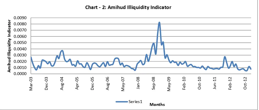
The Amihud ILLIQ indicator was aggregated for month specific analysis. The data very clearly

indicates that the Amihud ILLIQ was very high during financial crisis period and soon after as

liquidity dried up. However, the liquidity has improved considerably in recent months.

Amihud ILLIQ indicator was very high during financial crisis period indicating increasing

illiquidity in the market.

Table – 14: Descriptive Statistics for Amihud Illiquidity Indicator (Apr’03 –Feb’13)

Mean 0.001776

Standard Error 0.000105

Median 0.001501

Standard Deviation 0.001143

Sample Variance 1.31E-06

Kurtosis 10.49757

Skewness 2.736135

0.0000 0.0010 0.0020 0.0030 0.0040 0.0050 0.0060 0.0070 0.0080 0.0090 M ar -0 3 D e c-03 A ug -04 A pr -05 D e c-05 A ug -06 M ay -0 7 Jan -0 8 S e p-08 M ay -0 9 F e b-10 O ct -10 Jun -11 F e b-12 O ct -12 A m ihud Il li qui di ty Indi cat or Months Chart - 2: Amihud Illiquidity Indicator

Range 0.007697

Minimum 0.000538

Maximum 0.008235

Monthly Observations 119

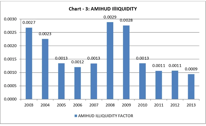
Year-wise analysis also indicates the drop in illiquidity after introduction of NDS-OM. As the

liquidity improved due to introduction of NDS-OM, this must have resulted in savings for all

market participants.

We wanted to test if there was any structural change in liquidity indicator after introduction on

NDSOM system and used the Chow test for testing the said information for a data period of 122

months (Jan’03 to Feb’13). The Aug’05 is the 32nd _{data point for which structural break is tested.}

We included change in yield and the lagged values of Amihud ILLIQ in the equation to test for

structural break significance.

Table – 15: Structural Change Test

Test Break Point Num DF Den DF F Value Pr > F Chow 32 4 113 7.8 <.0001

0.0027

0.0023

0.0013

0.0012 0.0013 0.0029

0.0028

0.0013

0.0011 0.0011 0.0009

0.0000 0.0005 0.0010 0.0015 0.0020 0.0025 0.0030

2003 2004 2005 2006 2007 2008 2009 2010 2011 2012 2013

Chart - 3: AMIHUD IllIQUIDITY

The Chow test very clearly indicated that there is a strong indication of structural break for data

point no. 32 (introduction of NDSOM system) as F-Values indicates statistical significance at

1% level.

The period of our study was divided into 3 groups – (a) PREOM period (from 01-Jan-2003 to

31-Jul-2005); (b) NDSOM – deals executed using the anonymous trading platform from

01-Aug-2005 to 28-Feb-2013; (c) NDS – the OTC deals reported to RBI NDS system from 01-Aug-2005

to 28-Feb-2013). We estimated the daily average ILLIQ ratio for each group. The results show

clearly that the liquidity has improved after introduction of NDSOM in both OTC as well as in

anonymous order driven market as the mean IILIQ in PREOM period was relatively higher

vis-à-vis the comparable values in post NDSOM. However, the volatility of ILLIQ has improved in

NDSOM market but not in the OTC market. The results change quite significantly if we take

only Government securities and drop other securities like T-Bills, SDLs, etc. The data for

NDS-OM falls short by 4 days as the representative trading was not available in NDS-NDS-OM platform

due to technical and other reasons while OTC trades were reported in NDS platform by traders.

When we consider all securities, we find that NDS-OM has marginally higher liquidity vis-à-vis

NDS system in post-NDSOM era. The transparency in NDS-OM system helped the market

participants to have better price discovery in OTC market.

Table -16: Amihud ILLIQUIDITY Indicators

GROUP DAYS Mean SDTDEV Skewness Kurtosis

All Securities

PREOM 756 0.0023 0.0026 3.8507 22.1883

NDS 1849 0.0017 0.0025 5.8015 56.5654

NDSOM 1845 0.0016 0.0019 4.0139 23.9587

Only Dated Govt. Securities

PREOM 756 0.0025 0.0029 4.1329 25.9236

NDS 1847 0.0019 0.0030 5.8240 57.7065

NDSOM 1845 0.0016 0.0020 3.9982 22.8242

Non-Dated Government Securities

PREOM 691 0.0011 0.0038 15.7713 319.5941

NDS 1449 0.0010 0.0026 6.6321 60.8577

However, all the tests showed that there is a statistically significant difference between the mean

of the variable Amihud ILLIQ and zero for all groups and it supports the relationship of price

impact and liquidity.

Annual average ILLIQ factor was estimated using the daily average ILLIQ for both NDS and

NDSOM transactions for all securities from 01-Aug-2005 to 28-Feb-2013. In most of the years,

ILLIQ factor for NDSOM has performed better vis-à-vis OTC NDS deals implying higher

liquidity in NDSOM vis-à-vis OTC NDS market. However, only in the initial phase of NDS-OM

(2005 & 2006), OTC NDS market had higher level of liquidity vis-à-vis NDS-OM.

Table – 17: Year-wise Amihud ILLIQ Indicator for all Securities

Year ILLIQ SDEV MAX MIN ILLIQ SDEV MAX MIN

PREOM

2003 0.00268 0.00334 0.02736 0.00021

2004 0.00225 0.00201 0.01941 0.00006 2005 0.00172 0.00178 0.01047 0.00008

NDS Market (01-Aug-2005 onwards) NDSOM Market (01-Aug-2005 onwards) 2005 0.00044 0.0003 0.00180 0.00007 0.00125 0.00158 0.01553 0.00014 2006 0.00104 0.00113 0.00814 0.00002 0.00141 0.00123 0.00769 0.00005 2007 0.00152 0.00304 0.04039 0.00000 0.00126 0.00133 0.01299 0.00008 2008 0.00351 0.00414 0.02544 0.00005 0.00257 0.00273 0.02147 0.00010 2009 0.00263 0.00326 0.03186 0.00016 0.00284 0.00302 0.01923 0.00000 2010 0.00149 0.00133 0.00882 0.00008 0.00125 0.00132 0.00985 0.00009 2011 0.00109 0.00101 0.00607 0.00003 0.00102 0.00112 0.01121 0.00004 2012 0.00108 0.00098 0.00625 0.00003 0.00107 0.00092 0.00505 0.00011 2013 0.00096 0.00074 0.00315 0.00005 0.00095 0.00048 0.00268 0.00026

Since NDSOM trading platform accounts for a lion’s share in dated Government securities while

major trading in SDL and T-bills are reported to NDS system, we estimated daily Amihud ILLIQ

factor by taking only Government dated securities into account. The result shows that in

Government securities, NDSOM significantly scores over trades reported in OTC NDS platform.

And in recent years, the liquidity in NDS-OM platform has increased significantly vis-à-vis the

Table – 18: Year-wise Amihud ILLIQ Indicator for Government Securities

Year ILLIQ SDEV MAX MIN ILLIQ SDEV MAX MIN

PREOM

2003 0.00278 0.00369 0.03179 0.00018

2004 0.00253 0.00230 0.02228 0.00007 2005 0.00210 0.00217 0.01695 0.00006

NDS Market (01-Aug-2005 onwards) NDSOM Market (01-Aug-2005 onwards)

Year ILLIQ SDEV MAX MIN ILLIQ SDEV MAX MIN

2005 0.00054 0.00039 0.00259 0.00008 0.00124 0.00158 0.01553 0.00014 2006 0.00126 0.00139 0.00840 0.00006 0.00138 0.00125 0.00794 0.00005 2007 0.00191 0.00384 0.05030 0.00000 0.00127 0.00128 0.01299 0.00008 2008 0.00414 0.00516 0.03134 0.00008 0.00259 0.00273 0.01702 0.00010 2009 0.00275 0.00344 0.03170 0.00022 0.00296 0.00328 0.02171 0.00000 2010 0.00153 0.00145 0.00882 0.00014 0.00119 0.00129 0.01108 0.00009 2011 0.00126 0.00135 0.01185 0.00002 0.00100 0.00114 0.01239 0.00004 2012 0.00118 0.00113 0.00692 0.00006 0.00100 0.00089 0.00505 0.00002 2013 0.00100 0.00085 0.00354 0.00007 0.00078 0.00044 0.00211 0.00026

We did a t-test (independent groups) to understand if the Amihud illiquidity factor is statistically

different in their mean for NDS and NDSOM platforms (taking all data). This t-test is designed

to compare means of same variable (Amihud ILLIQ) between two groups – NDS and

NDSOM. The p-value for the difference in means between NDS and NDS-OM is more than

0.05 for the entire period, so we conclude that the difference in means is not statistically

significantly different from 0. However, for the F-test (two-tailed significance probability), the

probability is less than 0.05. So there is evidence that the variances for the two groups, NDS and

NDSOM, are different. Therefore, we report Satterthwaite variance estimator for the t-test.

Satterthwaite is an alternative to the pooled-variance t-test and is used when the assumption that

the two populations have equal variances seems unreasonable. It provides a t-statistic that

asymptotically approaches a t distribution, allowing for an approximate t-test to be calculated

when the population variances are not equal.

The same t-test was extended to year-wise analysis. For 2005, 2006 and 2008, we find that the

difference in means of the variable ILLIQ for both NDS and NDSOM are statistically and

significantly different from 0 at 1% level and for 2010 the same is at 5% level. For other years,

statistically 0. The transparency in NDSOM has helped to improve liquidity in OTC market in

general. For 2005, 2007, 2008 and 2013, the F-test, p-values were significant at 1% evidencing

that the variances for the two groups are different. For other years, the test statistics are not

significant.

Table – 19: t-test results for Year-wise Amihud ILLIQ Indicator for all Securities

Mean Procedure t-Test Results F-Test Results

Sample Type N Mean Std Dev Std Err Method Variances DF t _Value Pr > |t| Equality of Variances

Full

NDS 1849 0.0017 0.0025 0.0001 Method Num _DF Den _DF F _Value Pr > F

NDSOM 1845 0.0016 0.0019 0.0000 Satterthwaite Unequal 3462.8 0.96 0.3346 Folded F* 1848 1844 1.7 <.0001

Diff (1-2) 0.0001 0.0022 0.0001 significant at 1%

2005

NDS 113 0.000436 0.0003 0.000028 Folded F* 112 112 27.74 <.0001

NDSOM 113 0.00125 0.00158 0.000149 Satterthwaite* Unequal 120.06 -5.37 <.0001 significant at 1%

Diff (1-2) -0.00081 0.00114 0.000151 significant at 1%

2006

NDS 246 0.00104 0.00113 0.000072 Pooled* Equal 490 -3.52 0.0005 Folded F 245 245 1.18 0.1855

NDSOM 246 0.00141 0.00123 0.000078

Diff (1-2) -0.00037 0.00118 0.000107 significant at 1%

2007

NDS 244 0.00152 0.00304 0.000194 Folded F* 243 243 5.17 <.0001

NDSOM 244 0.00126 0.00133 0.000085 Satterthwaite Unequal 333.54 1.21 0.2286 significant at 1%

Diff (1-2) 0.000256 0.00235 0.000212

2008

NDS 240 0.00351 0.00414 0.000267 Folded F* 239 240 2.3 <.0001

NDSOM 241 0.00257 0.00273 0.000176 Satterthwaite* Unequal 413.79 2.95 0.0033 significant at 1%

Diff (1-2) 0.000945 0.00351 0.00032 significant at 1%

2009

NDS 237 0.00263 0.00326 0.000212 Pooled Equal 472 -0.74 0.4607 Folded F 236 236 1.16 0.2538

NDSOM 237 0.00284 0.00302 0.000196

Diff (1-2) -0.00021 0.00314 0.000289

2010

NDS 246 0.00149 0.00133 0.000085 Pooled** Equal 490 1.97 0.0492 Folded F 245 245 1.01 0.9139

NDSOM 246 0.00125 0.00132 0.000084

Diff (1-2) 0.000235 0.00132 0.000119 significant at 5%

2011

NDS 240 0.00110 0.00101 0.000065 Pooled Equal 473 0.83 0.4054 Folded F 234 239 1.23 0.113

NDSOM 235 0.00102 0.00112 0.000073

Diff (1-2) 0.000081 0.00106 0.000097

2012

NDS 242 0.00108 0.000977 0.000063 Pooled Equal 482 0.11 0.9152 Folded F 241 241 1.12 0.3681

NDSOM 242 0.00107 0.000922 0.000059

Diff (1-2) 0.00001 0.00095 0.000086

NDSOM 41 0.000949 0.000478 0.000075 Satterthwaite Unequal 68.489 0.09 0.9271

significant at 1%

Diff (1-2) 0.000013 0.000622 0.000137

We did the same set of tests with Amihud ILLIQ taking into account only Government securities

and dropping T-Bills and other securities.The results are significantly different from the earlier

one (with all securities). When we considered only dated Government securities, we find that for

full period, the t-stat is significant at 1%. The p-value for the difference between NDS and

NDS-OM is less than 0.05 for the entire period, so we conclude that the difference in means is

statistically significantly different from 0. For the F-test (two-tailed significance probability), the

probability is less than 0.05. So there is evidence that the variances for the two groups, NDS and

NDSOM, are different. The same t-test was extended to year-wise analysis. For 2005, 2007,

2008 and 2010 we find that the difference in means of the variable ILLIQ are statistically

significantly different from 0 for both NDS and NDSOM at 1% level, for 2011 at 5% level and

for 2012 at 10% level. For other years, the p values are not significant and hence the mean is

statistically 0 for NDS and NDSOM. For 2005, 2007, 2008, 2011, 2012 and 2013, the F-test,

p-values were significant at 1% evidencing that the variances for the two groups are different. For

2006 and 2010, the same is significant at 10%. For only 2009, the test statistics are not

significant. Hence, NDSOM scores over NDS platform in term of liquidity when we consider

only Government securities.

Table – 20: t-test results for Year-wise Amihud ILLIQ Indicator for all Government Securities

Mean Procedure t-Test Results F-Test Results

Full

NDS 1847 0.00189 0.00299 0.00007 Folded _F* 1846 1844 2.26 <.0001

NDSOM 1845 0.00158 0.00199 0.000046 Satterthwaite* Unequal 3211.3 3.67 0.0002

significant at 1%

Diff (1-2) 0.000307 0.00254 0.000084

significant at 1%

2005

NDS 113 0.000539 0.000385 0.000036 Folded _F* 112 112 16.87 <.0001

NDSOM 113 0.00124 0.00158 0.000149 Satterthwaite* Unequal 125.23 -4.6 <.0001

significant at 1%

Diff (1-2) -0.0007 0.00115 0.000153

significant at 1%

2006

NDS 245 0.00126 0.00139 0.000089 Folded _F* 244 245 1.23 0.0998

NDSOM 246 0.00138 0.00125 0.00008 Satterthwaite Unequal 483.25 -0.98 0.3254

significant at 10%

Diff (1-2) -0.00012 0.00132 0.000119

2007

NDS 243 0.00191 0.00384 0.000246 Folded _F* 242 243 8.93 <.0001

NDSOM 244 0.00127 0.00128 0.000082 Satterthwaite* Unequal 295.32 2.46 0.0146

significant at 1%

Diff (1-2) 0.000638 0.00286 0.000259

2008

NDS 240 0.00414 0.00516 0.000333 Folded _F* 239 240 3.57 <.0001

NDSOM 241 0.00259 0.00273 0.000176 Satterthwaite* Unequal 362.92 4.12 <.0001

significant at 1%

Diff (1-2) 0.00155 0.00413 0.000376

significant at 1%

2009

NDS 237 0.00275 0.00344 0.000223 Pooled Equal 472 -0.66 0.5083 Folded

F

236 236 1.1 0.4786

NDSOM 237 0.00296 0.00328 0.000213

Diff (1-2) -0.0002 0.00336 0.000309

2010

NDS 246 0.00153 0.00145 0.000092 Folded _F*** 245 245 1.27 0.066

NDSOM 246 0.00119 0.00129 0.000082 Satterthwaite* Unequal 483.36 2.75 0.0062

significant at 10%

Diff (1-2) 0.00034 0.00137 0.000124

significant at 1%

2011

NDS 240 0.00126 0.00135 0.000087 Folded _F 239 234 1.41 0.0084

NDSOM 235 0.001 0.00114 0.000074 Satterthwaite** Unequal 462.63 2.3 0.0219

significant at 1%

Diff (1-2) 0.000264 0.00125 0.000115

significant at 5%

2012

NDS 242 0.00118 0.00113 0.000073 Folded _F* 241 241 1.63 0.0001

NDSOM 242 0.001 0.000886 0.000057 Satterthwaite* Unequal 455.55 1.92 0.055

significant at 1%

Diff (1-2) 0.000178 0.00102 0.000092

significant at 10%

2013

NDS 41 0.001 0.000846 0.000132 Folded _F* 40 40 3.78 <.0001

NDSOM 41 0.000785 0.000435 0.000068 Satterthwaite Unequal 59.785 1.46 0.1494

significant at 1%

Diff (1-2) 0.000217 0.000673 0.000149

As we have divided our trades into three different groups – liquid, semi-liquid and illiquid, we

wanted to test if there is any difference in liquidity for the same group of securities in different

platforms. We considered all securities for the analysis while calculating the Amihud ILLIQ

factor. Pre-NDSOM era had remarkably higher illiquidity.

Table – 21: Group-wise Amihud ILLIQ Indicator for all Securities

ILLIQUID LIQUID SEMI-LIQUID

Year _{ILLIQ SDEV MAX ILLIQ SDEV MAX ILLIQ SDEV MAX}

PREOM

2003 _{0.0048 0.0060 0.0433 0.0011 0.0014 0.0134 0.0032 0.0054 0.0571} 2004 _{0.0038 0.0050 0.0581 0.0009 0.0009 0.0055 0.0020 0.0018 0.0095} 2005 _{0.0027 0.0040 0.0297 0.0006 0.0006 0.0036 0.0016 0.0018 0.0106}

NDS - POSTOM

2013 _{0.0014 0.0013 0.0050 0.0011 0.0010 0.0050 0.0002 0.0002 0.0015}

NDSOM

2005 _{0.0032 0.0054 0.0424 0.0005 0.0004 0.0025 0.0014 0.0017 0.0129} 2006 _{0.0035 0.0039 0.0333 0.0005 0.0005 0.0041 0.0020 0.0020 0.0129} 2007 _{0.0036 0.0055 0.0445 0.0005 0.0005 0.0043 0.0016 0.0020 0.0160} 2008 _{0.0061 0.0111 0.1167 0.0009 0.0011 0.0130 0.0029 0.0035 0.0226} 2009 _{0.0059 0.0083 0.0567 0.0011 0.0016 0.0136 0.0033 0.0035 0.0247} 2010 _{0.0036 0.0073 0.0867 0.0003 0.0003 0.0019 0.0015 0.0018 0.0179} 2011 _{0.0028 0.0037 0.0335 0.0003 0.0003 0.0018 0.0016 0.0027 0.0290} 2012 _{0.0026 0.0033 0.0327 0.0003 0.0003 0.0020 0.0013 0.0014 0.0114} 2013 _{0.0023 0.0014 0.0071 0.0002 0.0002 0.0014 0.0011 0.0010 0.0056}

A graphical representation of the data clearly shows that OTC deals reported to NDS platform

has higher level of illiquidity for stocks classified as “Liquid” vis-à-vis securities classified as

“Illiquid” or “Semi-liquid”22.

We conducted similar analysis for dated Government securities and dropped all T-Bills, special

and State securities.

Table – 22: Group-wise Amihud ILLIQ Indicator for Government Securities

ILLIQUID LIQUID SEMI-LIQUID

Year ILLIQ SDEV MAX ILLIQ SDEV MAX ILLIQ SDEV MAX

PREOM

2003 _{0.0058 0.0079 0.0696 0.0011 0.0014 0.0134 0.0033 0.0058 0.0571} 2004 _{0.0049 0.0064 0.0811 0.0009 0.0009 0.0057 0.0024 0.0023 0.0189} 2005 _{0.0041 0.0056 0.0336 0.0006 0.0006 0.0036 0.0022 0.0023 0.0156}

NDS - POSTOM

2005 _{0.0002 0.0003 0.0028 0.0010 0.0007 0.0033 0.0004 0.0007 0.0070} 2006 _{0.0006 0.0006 0.0035 0.0031 0.0030 0.0188 0.0005 0.0005 0.0039} 2007 _{0.0009 0.0013 0.0114 0.0067 0.0084 0.0630 0.0005 0.0009 0.0070} 2008 _{0.0013 0.0020 0.0109 0.0126 0.0154 0.0924 0.0015 0.0025 0.0201} 2009 _{0.0021 0.0031 0.0261 0.0076 0.0121 0.0822 0.0015 0.0019 0.0123}

22 _{Illiq_L is for liquid securities; Illiq_IL if for illiquid securities and Illiq_sm is for Semi-liquid securities.} 0.0000 0.0020 0.0040 0.0060 0.0080 0.0100 0.0120 0.0140

2005 2006 2007 2008 2009 2010 2011 2012 2013

Chart - 4: NDS Platform - Amihud Illiquidity

ILLIQ_IL ILLIQ_L ILLIQ_SM

0.0000 0.0010 0.0020 0.0030 0.0040 0.0050 0.0060 0.0070

2005 2006 2007 2008 2009 2010 2011 2012 2013

Chart - 5: NDSOM Platform - Amihud Illiquidity