The Onset of Ferromagnetic Convection in a Micropolar
Ferromagnetic Fluid Layer Heated from Below
C. E. Nanjundappa1, I. S. Shivakumara2, K. Srikumar3
1Department of Mathematics, Ambedkar Institute of Technology, Bangalore, India; 2UGC-CAS in Fluid Mechanics, Department of Mathematics, Bangalore University, Bangalore, India; 3Department of Mathematics, East Point College of Engineering for Women, Bangalore, India.
Email: cenanju@hotmail.com
Received May 13th, 2012; revised June 20th, 2012; accepted July 10th, 2012
ABSTRACT
The onset of ferromagnetic convection in a micropolar ferromagnetic fluid layer heated from below in the presence of a uniform applied vertical magnetic field has been investigated. The rigid-isothermal boundaries of the fluid layer are considered to be either paramagnetic or ferromagnetic and the eigenvalue problem is solved numerically using the Galerkin method. It is noted that the paramagnetic boundaries with large magnetic susceptibility χ delays the onset of ferromagnetic convection the most when compared to very low magnetic susceptibility as well as ferromagnetic boundaries. Increase in the value of magnetic parameter M1 and spin diffusion (couple stress) parameter N3 is to hasten,
while increase in the value of coupling parameter N1 and micropolar heat conduction parameter N5 is to delay the onset
of ferromagnetic convection. Further, increase in the value of M1, N1, N5 and χ as well as decrease in N3 is to diminish
the size of convection cells.
Keywords: Micropolar Ferrofluid; Ferromagnetic Convection; Paramagnetic Boundaries; Rigid Boundaries; Magnetic Susceptibility
1. Introduction
Ferrofluids or magnetic fluids are commercially manu-factured colloidal liquids usually formed by suspending mono domain nanoparticles (their diameter is typically 3 - 10 nm) of magnetite in non-conducting liquids like heptane, kerosene, water etc. and they are also called mag- netic nanofluids. These fluids get magnetized in the pre- sence of an external magnetic field and due to their both liquid and magnetic properties they have emerged as reliable materials capable of solving complex engineer- ing problems. An extensive literature pertaining to this field and also the important applications of these fluids to many practical problems can be found in the books by Rosensweig [1], Berkovsky et al. [2] and Hergt et al. [3]. It is also recognized that these fluids have promising po- tential for heat transfer applications in electronics, micro and nanoelectromechanical systems (MEMS and NEMS), and air-conditioning and ventilation
Several theories were used to describe the motion of ferrofluids and amongst them the continuum description of the ferrofluids has been in existence since the work of Neuringer and Rosensweig [4]. Their theory is called “quasi-stationary theory”. Based on this theory, several studies on convective instability in a ferrofluid layer have
pre-dicted oscillatory instability in a certain region of mag-netic field and the fluid temperature. In a review article, Odenbach [13] has focused on recent developments in the field of rheological investigations of ferrofluids and their importance for the general treatment of ferrofluids.
The development of different kinds of ferrofluids ex- hibiting significant changes in their microstructure has outlined the need of new description for ferrofluids. It is believed that quasi-stationary theory is reasonably valid for colloidal suspensions of Néel particles in which the particle magnetic moment m rotates inside the particle and the particle does not rotate itself and hence no mo- mentum transfer, from the particle to the fluid, occurs when the applied magnetic field has a changing direction or magnitude. On the other hand, for Brownian particle in which the vector m is locked into the crystal axis of the particle and rotates along with the particle rotation, with finite magnetic relaxation time, one has to incorpo- rate the intrinsic rotation of the particle and there is thus momentum transfer to the carrier fluid in the form of a viscous friction. Based on these facts, the equations in- volving rotational or vortex viscosity and the nonequilib- rium magnetization equation, involving Brownian re-laxation time, are used to discuss thermoconvective in-stability of a ferrofluid in a strong external magnetic field by Stiles and Kagan [14]. However, more appropriate equations which allow proper consideration of internal rotation and vortex viscosity have been considered by Kaloni and Lou [15] to investigate convective instability problem in the horizontal layer of a magnetic fluid with Brownian relaxation mechanism. Recently, Paras Ram and Kushal Sharma [16] have studied the effect of mag- netic field-dependent viscosity (MFD) along with poros- ity on the revolving Axi-symmetric steady ferrofluid flow with rotating disk.
Since the ferrofluids are colloidal suspensions of nano- particles, as suggested by Rosensweig [1] in his mono- graph, it is pertinent to consider the effect of microrota- tion of the particles in the study. Based on this fact, stud-ies have been undertaken by treating ferrofluids as mi-cropolar fluids and the theory of mimi-cropolar fluid pro-posed by Eringen [17] has been used in investigating the problems. Micropolar fluids have been receiving a great deal of interest and research focus due to their applica- tions like solidification of liquid crystals, the extrusion of polymer fluids, cooling of a metallic plate in a bath col- loidal suspension solutions and exotic lubricants. In the uniform magnetic field, the magnetization characteristic depends on particle spin but does not on fluid velocity: Hence micropolar ferrofluid stability studies have be- come an important field of research these days. Although convective instability problems in a micropolar fluid layer subject to various effects have been studied exten- sively, the works pertaining to micropolar ferrofluids is
in much-to-be desired state. Many researchers [18-23] have been rigorously investigated the Rayleigh-Benard situation in Eringen’s micropolar non-magnetic fluids. From all these studies, they mainly found that stationary convection is the preferred mode for heating from below. Sharma and Kumar [24] and Sharma and Gupta [25] also gave a good understanding of thermal convection of mi-cropolar fluids. Zahn and Greer [26] have considered in- teresting possibilities in a planar micropolar ferromag- netic fluid flow with an AC magnetic field. They have examined a simpler case where the applied magnetic fields along and transverse to the duct axis are spatially uniform and varying sinusoidally with time. Abraham [27] has investigated the problem of Rayleigh-Benard convection in a micropolar ferromagnetic fluid layer per- meated by a uniform magnetic field for stress-free boun- daries. Reena and Rana [28,29] have studied the some convection problems on micropolar fluids saturating a porous medium. Recently, Thermal instability problem in a rotating micropolar ferrofluid has also been considered by Qin and Kaloni [30] and Sunil et al. [31], and refer- ences therein.
However, the increased importance of ferrofluids in many heat transfer applications demand the study of the onset of ferromagnetic convection in a layer of micropo-lar ferrofluid for more realistic velocity and magnetic boundary conditions. The aim of the present paper is, therefore, to investigate the onset of ferromagnetic con-vection in a micropolar ferrofluid layer heated from be- low in the presence of a uniform vertical magnetic field by considering the bounding surfaces as rigid- isothermal and which are either paramagnetic or ferromagnetic. The resulting eigenvalue problem is solved numerically using the Galerkin technique. The critical thermal Rayleigh number and associated wave number account for the sta-bility character.
2. Mathematical Formulation
The physical configuration considered is as shown in Figure 1. We consider an initially quiescent horizontal incompressible micropolar ferrofluid layer of character-istic thickness in the presence of an applied uniform magnetic field 0
d
H in the vertical direction with the an- gular momentum . The lower and the upper bounda-ries are rigid-isothermal which are either paramagnetic or ferromagnetic. Let 0 and be the tempera-
tures of the lower and upper rigid boundaries, respec- tively with
ω
T T1
T0
0T1
being the temperature dif- ference. A Cartesian co-ordinate systemT T
x y z, ,
is used with the origin at the bottom of the layer and z-axis is directed vertically upward. Gravity acts in the negative z-direction, g gkˆ where is the unit vector in the z-direction.Figure 1. Physical configuration.
In the above equations, is the velocity of the fluid, the pressure,
, , u v w
q
The basic equations governing the motion of an in-compressible Boussinesq micropolar ferromagnetic fluid for the above model are as follows [1,6,17,30]:
Continuity equation
0.
q (1) Angular momentum equation
0 2 2 r r p t qq q g B H
q ω
.(2)
Internal angular momentum equation
0 0 2 2 2 . r I t ω q ω q ω M H
ω ω
p the density, the shear kinematic viscosity co-efficient, r the vortex (rota-tional) viscosity, ω
1, 2, 3
the angular (average spin) velocity of colloidal particles along z-axis, I the moment of inertia, 0 the reference density, 0 thefree space magnetic permeability, the shear spin viscosity co-efficient, k1 the thermal conductivity, T
the temperature, the thermal expansion co-efficient,
the micropolar heat conduction coefficient, V H,
the specific heat at constant volume and magnetic field, the magnetic induction field,
C
B H the magnetic field,
H the magnitude of H, H0 the constant applied
magnetic field,
0 0,
H T the pyromagnetic co-efficient, the magnetization,
K M T
M M the magnitude
of M, M0M H T
0, 0
the constant mean value of
(3) magnetization,
H0, 0T
M H
Energy equation
0 , 0 0
, ,
2
1 .
V H
V H V H
DT D
C T
T Dt T D
k T T
M M t H ω H
the magnetic suscep- tibility, the magnetic potential and
2 2 x2 2 y2 2 z2
is the Laplacian opera-tor.
(4)
The basic state is quiescent and is given by
2 0 0 0
2 2 2
0 0 0
2
2
1 2 1
b
gz
p z p gz
M K z K z
Equation of state
0 1 T T
0 . (5)
Maxwell’s equation in the magnetostatic limit
0b
T z T z
0
B , H0 or H (6a,b)
0 1 0
b Tb T
0 .
B M H
(7) It is considered that the magnetization is aligned with the magnetic field and is taken as a function of both magnetic field and temperature in the form
0
1
ˆb
K z
z H
k H
,
.M H T H
H
M (8)
0 1 ˆ
b
K z
z M
k
M (10)
The magnetic equation of state is given by
where, T d is the temperature gradient and the subscript b denotes the basic state.
0 0 0
.To study the stability of the system, the variables are perturbed in the form
, , , , b b b bq p p z p T T z
z q ω
H H H M M M
, T
(11)
where, q,, , p, T, H and M are the perturbed quantities whose magnitude is assumed to be very small.
Substituting Equation (11) in Equation (6a) and using Equations (8) and (9) and assuming K z
1
H0as propounded by Finlayson [6], we obtain (after drop-ping the primes)
0 0
0 0
1 , 1
1
,
x x x y y
z z z
M M
y
M H H M H
H H
M H H KT
H (12)
where
H H Hx, y, z
and
M M Mx, y, z
are the
x y z, ,
components of the magnetic field and mag-netization respectively.Using Equation (11) in Equation (2) and linearizing, we obtain (after dropping primes)
2
0 1
1
0 0 0
2
r r
u p u
t x H M H z (13)
2 0 20 0 0
2 r r v p v t y H M H z 2 (14)
2 0 3 30 0 0 0
2 0 0 3 2 . 1 r r w p w t z H M H z K T K H gT
(15)
Differentiating Equations (13)-(15) partially with re-spect to x, y and z respectively and adding, we get
2 2
0 0 0
2 2
0
0 (1 ) 0 2
p M H
z K T g K z z (16)
Eliminating the pressure term from Equation (15), using Equation (16) we get
p
2 2 2
0 0
2
2 2
0
0 2 3
1 r h h r w K t z K g T
where, 2 2 2 2 2
h x y
is the horizontal
Lapla-cian operator.
Substituting Equation (11) into Equation (3) and lin-earizing, we obtain (after dropping primes)
2 2
3
0I t 2 r w 2 3 3
.
(18)
As before, substituting Equation (11) into Equation (4) and linearizing, we obtain (after dropping primes)
22 0 0
0 0 1 0 0
0 0 3
1 T K
C k T C
t T K t z w (19)
where, 0C00CV H, 0KHb. Finally Equations (6), after using Equation (12), yield (after dropping primes)
2 0 22
0
1 1 h 0
M T K H z z .
(20)
The principle of exchange of stability is assumed and the normal mode expansion of the dependent variables is taken in the form
3 3
, , , , , ,
exp i
w T W z z z z
lx my
(21)
where, and l mare the wave numbers in the xand directions, respectively.
y
Let us non-dimensionalize the variables by setting
x y z, ,
x y z, ,d d d
, DDd, aad,
d W W , d ,
2 2 1 K d , 33 3,
d
I 12I
d
(22)
where, 0 is the kinematic viscosity and 1 0 0
k C
is the thermal diffusivity. Equation (21) is substituted into Equations (17)-(20) and then Equation (22) is used to obtain the stability equations in the fol-lowing form:
2
2 2 2
1 1 2 2 1 3 1 1 2 0 t
N D a W a R M D M
N D a
1
(23)
2 2
2 2
1 3 3
2N D a W 2 N D a
(17)
3 0
(24)
2 2
2 5 3
1 0
D a M W N (25)
2 2
3 0
2
a m2 is the horizontal wave number, 4
t
R gd is the thermal Rayleigh number,
2
1 0 1 0
M K g is the magnetic number,
22 0 0 1 0 0
M T K C is the magnetic parameter,
3 1 0 0 1
M M H is the non-linearity of mag-netization, N1 r is the coupling parameter,
2 3
N d is the spin diffusion (couple stress)
pa-rameter and 2
5 0 0
N Cd is the micropolar heat conduction parameter. The typical value of M2 for
magnetic fluids with different carrier liquids turns out to be of the order of and hence its effect is neglected when compared to unity.
6
10
Equations (23)-(26) are solved using the following boundary conditions:
i) Both boundaries rigid-isothermal and paramagnetic
3
0 , 0, 0 at 0
W DW z ,1 (27a)
1 , at 0
1 , at 1
a z D a z . ,1 , z (27b)
ii) Both boundaries rigid-isothermal and ferromag-netic
3
0 , 0, 0, 0 at 0
W DW z . (27c)
3. Numerical Solution
Equations (23)-(26) together with the boundary condi-tions (27a,b) or (27c) constitute an eigenvalue problem with the thermal Rayleigh number t as the eigenvalue. For the boundary conditions considered, it is not possible to obtain the solution to the eigenvalue problem in closed form and hence it is solved numerically using the Galer- kin-type weighted residuals method. Accordingly, the va- riables are written in a series of basis functions as
R
3 3 1 1 1 1 , , ( ) N Ni i i i
i i
N N
i i i i
i i
W z AW z C z
z D z z E
(28)where, Ai, i, i and i are the unknown con-stants to be determined. The basis functions
C D E
i
W z ,
3i , i and i are generally chosen such
that they satisfy the corresponding boundary conditions but not the differential equations. Substituting Equation (28) into Equations (23)-(26), multiplying the resulting momentum equation by
z
z
z
,j
W z angular momentum equation by 3j
z , temperature equation by j
zand the magnetic potential equation by j
z ;per-forming the integration by parts with respect to z between z = 0 and z = 1 and using the boundary conditions (27a,b) or (27c), we obtain the following system of 4n linear homogeneous algebraic equations in the 4n unknowns
i
A , Ci, Di and Ei; i1, 2, , : n
jiCi E Dji i 0
ji i ji i
C A D F E
0 jiEi
(29)
ji i
G A H
0
i ji i
C K E
(30)
ji i
I A Jji
0. i D
(31)
ji i i
L C Pj (32) The coefficients CjiPji involve the inner products of the basis functions and are given by
2 21
C N
a D2 4
1
2
j i
j i j i
D W D W
W DW a W W
ji
2 1 1ji Rt j i
D a M W
2 1
ji t j i
E a R M W D
2
1 3
2 j i j 3i
Fji N DW D a W
2
1 3 3
2
ji j i j i
G N D DW a W
1 3 3 2
3 3 3 3 3
4
ji j i
j i j i
H N
N D D a
1 2
ji j i
I M W
2
ji j i j i
J D D a
5 3
ji j
K N i
ji j
L D i
2 32 1
ji j i
a
P D D a M
j i
(33)
where the inner product is defined as
1
0
d .z
The above set of homogeneous algebraic equations can have a non-trivial solution if and only if
0 0
0. 0
0 0
ji ji ji ji
ji ji
ji ji ji
ji ji
C D E F
G H
I J K
L P
(34)
The eigenvalue has to be extracted from the above characteristic equation. For this, we select the trial func-tions as follows:
Case i): Rigid-paramagnetic boundaries
4 3 2 2
1 3 1
2
1 1
2 ,
, 1 2
i i i
i i i i
W z z z T z z T
z z T z T
Case ii): Rigid-ferromagnetic boundaries
4 3 2 2
1 3 1
2 2
1 1
2 ,
,
i i i
i i i i
W z z z T z z T
z z T z z T
i ,
(36)
where are the modified Chebyshev polynomials. It may be noted that the trial function i does not sat-isfy the corresponding boundary conditions in the case of paramagnetic boundaries but the residual technique is used for the function (see [6]) and the first term on the right hand side of
'
i
T s
i
ji represents the residual term. In the case of ferromagnetic boundaries, i satisfies the corresponding boundary conditions and hence pre-vents the use of residual technique. Then the coefficient
P
ji
P is given by
2 3
ji D jD i a M j
P
i
. (37)
The characteristic Equation (34) is solved numerically for different values of physical parameters using the Newton-Raphson method to obtain the Rayleigh number
t as a function of wave number and the bisection method is built-in to locate the critical stability parame-ters to the desired degree of accuracy.
R a
R atc, c4. Results and Discussion
The classical linear stability analysis has been carried out to investigate the onset of ferromagnetic convection in a horizontal micropolar ferrofluid layer. The lower and upper boundaries are considered to be rigid-isothermal which are either paramagnetic or ferromagnetic. The critical thermal Rayleigh number and the corre-sponding wave number
are used to characterize the stability of the system. The critical stability parame-ters computed numerically by the Galerkin method as explained above, are found to converge by considering nine terms in the Galerkin expansion. To validate the numerical solution procedure used, a new magnetic pa-rameter independent of the temperature gradient, was introduced in the form
Rtc
ca
, S
2 ,
m t
R R S where
2 2d4 20 0
1
S g K
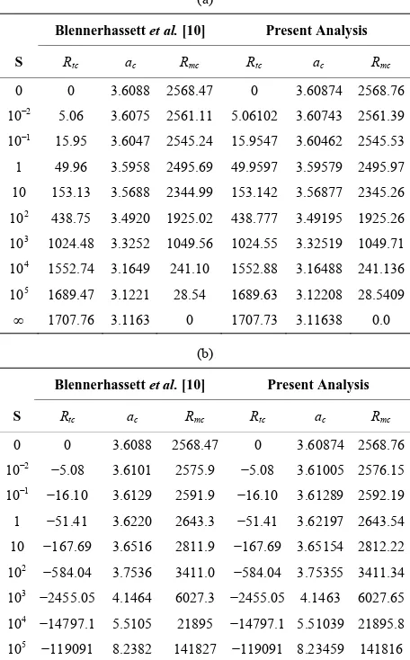
. The critical thermal Ra- yleigh number , critical magnetic Rayleigh number and the corresponding wave number com- puted numerically in the absence of micropolar effects are compared in Table 1 with the previously published results of Blennerhassett et al. [8]. It is seen that our results for different values of are in good agreement. Also, it is instructive to know the proc-esses of convergence of results as the number of terms in the Galerkin approximation increases for the problem considered. Hence, various levels of the approximations to the critical thermal Rayleigh number tc and the corresponding wave number are also obtained for
differ-ent values of when ,
Rtc50
1
N
RmcN N
acS
R
1
m tM
1 3N3 1,
[image:6.595.309.537.138.505.2]M R R 100
Table 1. Comparison of Rtc and Rmc for different values of S with N1 = N3 = N5 = 0 (i.e., in the absence of micropolar effect).(a) When heated from below; (b) When heated from above.
(a)
Blennerhassett et al. [10] Present Analysis
S Rtc ac Rmc Rtc ac Rmc
0 0 3.6088 2568.47 0 3.60874 2568.76 10−2 5.06 3.6075 2561.11 5.06102 3.60743 2561.39
10−1 15.95 3.6047 2545.24 15.9547 3.60462 2545.53
1 49.96 3.5958 2495.69 49.9597 3.59579 2495.97 10 153.13 3.5688 2344.99 153.142 3.56877 2345.26 102 438.75 3.4920 1925.02 438.777 3.49195 1925.26
103 1024.48 3.3252 1049.56 1024.55 3.32519 1049.71
104 1552.74 3.1649 241.10 1552.88 3.16488 241.136
105 1689.47 3.1221 28.54 1689.63 3.12208 28.5409
∞ 1707.76 3.1163 0 1707.73 3.11638 0.0
(b)
Blennerhassett et al. [10] Present Analysis
S Rtc ac Rmc Rtc ac Rmc
0 0 3.6088 2568.47 0 3.60874 2568.76 10−2 −5.08 3.6101 2575.9 −5.08 3.61005 2576.15
10−1 −16.10 3.6129 2591.9 −16.10 3.61289 2592.19
1 −51.41 3.6220 2643.3 −51.41 3.62197 2643.54 10 −167.69 3.6516 2811.9 −167.69 3.65154 2812.22
102 −584.04 3.7536 3411.0 −584.04 3.75355 3411.34
103 −2455.05 4.1464 6027.3 −2455.05 4.1463 6027.65
104 −14797.1 5.5105 21895 −14797.1 5.51039 21895.8
105 −119091 8.2382 141827 −119091 8.23459 141816
3 2
N , N51 and the results are tabulated in Table 2
for different types of magnetic boundary conditions. It is seen that with an increase in the number of terms in the Galerkin approximation, goes on decreasing and finally for the order tc
R 9 i j
N
R
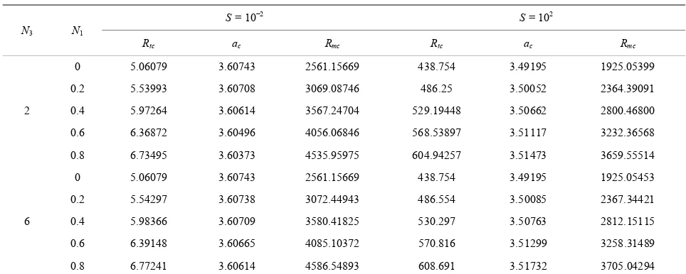
the results converge. This clearly demonstrates the accuracy of the numerical pro-cedure employed in solving the problem. The critical values obtained for different values of 1 and as
well as for two values of 3 and 6 are exhibited in
Table 3. It may be noted that as S increases the magnetic Rayleigh number m decreases, while the value of the critical Rayleigh number tc increases. This implies that, in some favorable circumstances it is possible for the magnetic mechanism alone to induce convection.
N S
2
R
The neutral stability curves ( t againsta) for differ-ent values of 1
R
M , 1, 3 and 5 are shown
respec-tively in Figures 2-5 for paramagnetic/ferromagnetic boundaries. The neutral curves exhibit single but
Table 2. Critical values of Rtc and ac for different values of N1 when M31, Rm100, N32 and : (a) Para-
magnetic boundaries when
N51 1 8; (b) Paramagnetic boundaries when 0; (c) Ferromagnetic boundaries.
(a)
i = j = 1 i = j = 3 i = j = 5 i = j = 8 i = j = 9 N1
Rtc ac Rtc ac Rtc ac Rtc ac Rtc ac
0 1692.812 3.14012 1658.586 3.14784 1658.084 3.14792 1658.083 3.14792 1658.083 3.14792
0.2 2529.982 3.11900 2495.969 3.13195 2495.065 3.13204 2495.064 3.13205 2495.064 3.13205
0.4 3821.487 3.08148 3813.226 3.10318 3811.682 3.10335 3811.681 3.10336 3811.681 3.10336
0.6 6049.422 3.00816 6166.736 3.04365 6164.059 3.04397 6164.060 3.04397 6164.060 3.04397
0.8 10707.379 2.84549 11477.222 2.89729 11472.309 2.89794 11472.317 2.89794 11472.317 2.89794
(b)
i = j = 1 i = j = 3 i = j = 5 i = j = 8 i = j = 9 N1
Rtc ac Rtc ac Rtc ac Rtc ac Rtc ac
0 1673.024 3.12985 1644.147 3.13635 1643.612 3.13648 1643.611 3.13649 1643.611 3.13649
0.2 2510.090 3.11210 2481.449 3.12425 2480.512 3.12438 2480.511 3.12439 2480.511 3.12439
0.4 3801.401 3.07695 3798.544 3.09814 3796.967 3.09833 3796.966 3.09834 3796.966 3.09834
0.6 6028.949 3.00539 6151.699 3.04056 6148.990 3.04090 6148.991 3.04090 6148.991 3.04090
0.8 10686.048 2.84409 11461.278 2.89572 11456.336 2.89637 11456.344 2.89637 11456.344 2.89637
(c)
1
i j i j 3 i j 5 i j 8 i j 9
N1
Rtc ac Rtc ac Rtc ac Rtc ac Rtc ac
0 1649.975 3.11652 1628.295 3.12105 1627.728 3.12124 1627.727 3.12124 1627.727 3.12124
0.2 2486.932 3.10307 2465.523 3.11397 2464.554 3.11414 2464.553 3.11415 2464.553 3.11415
0.4 3778.005 3.07093 3782.424 3.09135 3780.815 3.09157 3780.815 3.09157 3780.815 3.09157
0.6 6005.043 3.00158 6135.118 3.03633 6132.378 3.03668 6132.380 3.03668 6132.380 3.03668
[image:7.595.56.538.540.733.2]0.8 10660.918 2.84198 11443.449 2.89346 11438.477 2.89411 11438.485 2.89411 11438.485 2.89411
Table 3. Critical values of Rtc and Rmc for different values of N1 with M31 and N51.
S = 10−2 S = 102
N3 N1
Rtc ac Rmc Rtc ac Rmc
0 5.06079 3.60743 2561.15669 438.754 3.49195 1925.05399
0.2 5.53993 3.60708 3069.08746 486.25 3.50052 2364.39091
0.4 5.97264 3.60614 3567.24704 529.19448 3.50662 2800.46800
0.6 6.36872 3.60496 4056.06846 568.53897 3.51117 3232.36568 2
0.8 6.73495 3.60373 4535.95975 604.94257 3.51473 3659.55514
0 5.06079 3.60743 2561.15669 438.754 3.49195 1925.05453
0.2 5.54297 3.60738 3072.44943 486.554 3.50085 2367.34421
0.4 5.98366 3.60709 3580.41825 530.297 3.50763 2812.15115
0.6 6.39148 3.60665 4085.10372 570.816 3.51299 3258.31489 6
different minimum with respect to the wave number and their shape is identical in the form to that of Benard problem in a micropolar fluid layer. For increasing M1
(see Figure 2), (see Figure 3), 5 (see Figure 4)
and decreasing 3 (see Figure 5), the neutral curves
are slanted towards the higher wave number region. From the figures, it is also seen that increasing
1
N N
N
is to
shift the neutral curves towards the higher wave number region. Moreover, the effect of increasingM1 and 3
as well as decreasing , and
N
1
N N5 is to decrease the
[image:8.595.138.458.184.441.2] [image:8.595.143.454.466.714.2]region of stability.
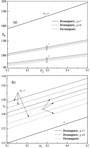
Figure 6(a) represents the variation of critical Ray- leigh number tc as a function of for different values of
R
1
1
N
M and for M35, N32 and
2 3 4 5
600 1200 1800 2400
a
Paramagnetic, = 7
Paramagnetic, =0
Ferromagnetic
Rt
M1=0
1
2
Figure 2. Neutral curves for different values of M1 when M35, N10.2, N32 and N50.5.
2 3 4 5
500 750 1000 1250 1500
Paramagnetic, = 7
Paramagnetic, =0
Ferromagnetic
Rt
N1=0.5
0.2
0
a
3 4 750
775 800 825 850
4.25 4
6 N3=2
Rt
Paramagnetic, = 7
Paramagnetic, =0
Ferromagnetic
a
[image:9.595.141.460.82.342.2]2.4
Figure 4. Neutral curves for different values of N3 when M12, M35, N10.2 and N50.5.
3 4
750 800 850
4.25 2.3
740
0 0.2
N5=0.5
Paramagnetic, = 7
Paramagnetic, =0
Ferromagnetic
Rt
a
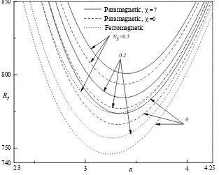
Figure 5. Neutral curves for different values of N3 when M12, M35, N10.2 and N32.
5 for both ferromagnetic and paramagnetic
boundary conditions. It is seen that tc decreases with an increase in the value of 1
0.5 N
R
M and hence its effect is to hasten the onset of ferroconvection due to an increase in the destabilizing magnetic force and the curve for
1 corresponds to non-magnetic micropolar fluid
case. In other words, heat is transported more efficiently
in magnetic fluids as compared to ordinary micropolar fluids. Also observed that tc increases with increasing
1. This is because, as 1 increases the concentration
of microelements also increases and as a result a greater part of the energy of the system is consumed by these elements in developing gyrational velocities in the fluid which ultimately leads to delay in the onset of
ferromag-0
M
[image:9.595.143.456.369.620.2]netic convection. Moreover, the system is found to be more stable if the boundaries are paramagnetic with
7
as compared to the case of 0 and the sys-tem is least stable if the boundaries are ferromagnetic. A closer inspection of the figure further depicts that the deviation in the tc values for different magnetic boun- dary conditions is more pronounced with increasing cou-pling parameter. In Figure 6(b) plotted the critical wave
number as a function of 1. It is evident that
in-creasing 1
R
c
a N
N
, and M1 is to increase the value of c and thus their effect is to reduce the dimension of the
convection cells.
a
In Figure 7(a) plotted tc as a function of 1 for
different values of spin diffusion (couple stress) parame-ter 3 when 1
R N
N M 2, 3 and 5 . Here, it
is observed that curves for different coalesce
5
0.5
M N 0.5
3
N
tc
R
0.1 .2 0.
1000 1500 2000 2500
0 3 0.4
Paramagnetic,= 7
Paramagnetic,= 0
Ferromagnetic
Rtc
N1
2850
(a)
2 1 M1=0
580
0.1 0.2 0.3 0.4 0.5
3.15 3.22 3.29 3.36 3.43
M1=2
1 3.48
0
ac
N1
(b)
Paramagnetic,= 7
Paramagnetic,= 0
[image:10.595.143.452.193.700.2]Ferromagnetic
Figure 6. Variation of (a) Rtc and (b) acas a function of N1 for different values of M1 when M35, N32 and
.
5 0.5
when 1 The impact of 3 on the stability
char-acteristics of the system is noticeable clearly with in-creasing 1 and then it is seen that the critical Rayleigh
number decreases with increasing indicating the spin diffusion (couple stress) parameter 3 has a
destabiliz-ing effect on the system. This may be attributed to the fact that as 3 increases, the couple stress of the fluid
in-creases, which leads to a decrease in microrotation and hence the system becomes more unstable. Figure 7(b) illustrates that increase in 1 and decrease in 3 for
non-zero values of 1 is to increase ac and hence
their effect is to decrease the size of convection cells.
0. N
N
N
N
3
N N
N N
N
The variation of critical thermal Rayleigh number
as a function of 1 for different values of 5 for 1
tc
R
N N
2
M , M35 and N32 is shown in Figure 8(a).
It is observed that increasing micropolar heat conduction parameter always has a stabilizing effect for nonzero values of 1 When 5 increases, the heat induced into
microelements of the fluid is also increased, thus decreas-ing the heat transfer from the bottom to the top. This de-crease in heat transfer is responsible for delaying the onset of ferromagnetic convection. Figure 8(b) illustrates that increase in 1 and 5 is to increase c and hence
their effect is to decrease the size of convection cells.
5
N . N
N
tc
R N
N a
Figure 9 shows the locus of the critical thermal Ray- leigh number and the critical magnetic Rayleigh
0.1 0.2 0.3 0.4 0.5
700 800 900 1000 1100
6 4
N3=2
650 Rtc
N1 Paramagnetic,= 7
Paramagnetic,= 0
Ferromagnetic
(a)
0.1 0.2 0.3 0.4 0.5
3.24 3.30 3.36 3.42 3.47
6
4 N3=2
Paramagnetic,= 7
Paramagnetic,= 0
Ferromagnetic
ac
N1 (b)
3.22
Figure 7. Variation of (a) Rtc and (b) acas a function of N1 for different values of N3 when M12, M35 and
.
5 0.5
[image:11.595.161.433.251.701.2]0.1 0.2 0.3 0.4 0.5 700
800 900 1000
Paramagnetic,= 7
Paramagnetic,= 0
Ferromagnetic
1050
0 N5=0.5
670
Rtc
(a)
N1
0.1 0.2 0.3 0.4 0.5
3.24 3.30 3.36 3.42
0 3.47
3.20
N5=0.5
ac
(b)
N1
Paramagnetic,= 7
Paramagnetic,= 0
[image:12.595.151.445.86.579.2]Ferromagnetic
Figure 8. Variation of (a) Rtc and (b) acas a function of N1 for different values of N5 for M12, M35 and
.
3 2
N
mc for 3 1 3 and 5
R M 5,N 0.2,N 2 N 0.5. In the figure, the regions above and below the curves, corre- spond, respectively, to unstable and stable ones. It is ob- served that there is a strong coupling between the critical thermal Rayleigh and the magnetic Rayleigh numbers such that an increase in the one decreases the other. Thus, when the buoyancy force is predominant, the magnetic force becomes negligible and vice-versa. The stability curves are slightly convex and in the absence of buoyancy forces
Rtc0
, the instability sets in at higher values ofmc indicating the system is more stable when the mag- netic forces alone are present. The stability region in- creases with increasing
R
and also for paramagnetic boundaries when compared to ferromagnetic boundaries.
5. Conclusions
0 600 1200 1800 2400 0
500 1000 1500 2000
2750
Paramagnetic, = 7 Paramagnetic, =0
... Ferromagnetic
Rtc
Rmc
[image:13.595.145.450.86.329.2]2150
Figure 9. Locus of Rtc and Rmc for M35, N10.2, N32 and N50.5.
uniform applied vertical magnetic field for more realistic rigid boundary conditions which are considered to be either paramagnetic or ferromagnetic. The resulting ei-genvalue problem is solved numerically by employing the Galerkin method.
From the foregoing study, the following conclusions may be drawn:
i) The neutral stability curves for various values of physical parameters exhibit that the onset of ferromag-netic convection retains its unimodal shape with one dis-tinct minimum which defines the critical thermal Ray- leigh number and the corresponding wave number.
ii) The system is more stabilizing against the ferro-magnetic convection if the boundaries are paraferro-magnetic with high magnetic susceptibility and least stable if the boundaries are ferromagnetic. It is observed that
0 0
rigid-ferromagnetic
and and
and
tc c tc c
tc c
R a R a
R a
.
iii) The effect of increasing the value of magnetic number M1 is to hasten the onset of ferromagnetic
convection.
iv) The effect of increasing the value of coupling pa-rameter 1 and micropolar heat conduction parameter
5 is to delay, while increasing the spin diffusion
(cou-ple stress) parameter is to hasten the onset of fer-romagnetic convection.
N N
3
N
v) The effect of increasing N1, N5, and M1as
well as decrease in is to increase the critical wave
number. 3
N
vi) The magnetic and buoyancy forces are
comple-mentary with each other and the system is more stabiliz-ing when the magnetic forces alone are present.
6. Acknowledgements
The work reported in this paper was supported the Man-agement (Panchajanya Vidya Peetha Welfare Trust) and Principal of Dr. Ambedkar Institute of Technology and East Point College of Engineering for Women, Banga-lore for the encouragement.
REFERENCES
[1] R. E. Rosensweig, “Ferrohydrodynamics,” Cambridge Uni- versity Press, London, 1985.
[2] B. M. Berkovsky, V. F. Medvedev and M. S. Krakov, “Magnetic Fluids, Engineering Applications,” Oxford Uni- versity Press, Oxford, 1993.
[3] R. Hergt, W. Andrä, C. G. Ambly, I. Hilger, U. Richter and H. G. Schmidt, “Physical Limitations of Hypothermia Using Magnetite Fine Particles,” IEEE Transictions of Magnetics, Vol. 34, No. 5, 1998, pp. 3745-3754.
doi:10.1109/20.718537
[4] J. L. Neuringer and R. E. Rosensweig, “Magnetic Fluids,” Physics of Fluids, Vol. 7, No. 12, 1964, pp. 1927-1937. doi:10.1063/1.1711103
[5] B. A. Finlayson, “Convective Instability of Ferromagnetic Fluids,” Journal of Fluid Mechanics, Vol. 40, No. 4, 1970, pp. 753-767. doi:10.1017/S0022112070000423
[6] K. Gotoh and M. Yamada, “Thermal Convection in a Ho- rizontal Layer of Magnetic Fluids,” Journal of Physics, Society of Japan, Vol. 51, 1982, pp. 3042-3048.
[7] P. J. Stiles, F. Lin and P. J. Blennerhassett, “Heat Trans- fer through Weakly Magnetized Ferrofluids,” Journal of Colloidal and Interface Science, Vol. 151, No. 1, 1992, pp. 95-101. doi:10.1016/0021-9797(92)90240-M
[8] P. J. Blennerhassett, F. Lin and P. J. Stiles, “Heat Trans- fer through Strongly Magnetized Ferrofluids,” Proceed-ing of Royal Society A: A Mathematical, Physical and En- gineering Sciences, Vol. 433, 1991, pp. 165-177.
[9] Sunil and A. Mahjan, “A Nonlinear Stability Analysis for Magnetized Ferrofluid Heated from Below,” Proceeding of Royal Society of London. A Mathematical, Physical and Engineering Sciences, Vol. 464, No. 2089, 2008, pp. 83-98. doi:10.1098/rspa.2007.1906
[10] C. E. Nanjundappa and I. S. Shivakumara, “Effect of Velocity and Temperature Boundary Conditions on Con- vective Instability in a Ferrofluid Layer,” ASME Journal of Heat Transfer, Vol. 130, 2008, Article ID: 104502. [11] M. I. Shliomis, “Convective Instability of Magnetized
Ferrofluids: Influence of Magneto-Phoresis and Soret Ef- fect,” Thermal Non-Equilibrium Phenomena: Fluid Mix- tures, Vol. 584, 2002, pp. 355-371.
[12] M. I. Shliomis and B. L. Smorodin, “Convective Instabil- ity of Magnetized Ferrofluids,” Journal of Magnetism and Magnetic Materials, Vol. 252, 2002, pp. 197-202. doi:10.1016/S0304-8853(02)00712-6
[13] S. Odenbach, “Recent Progress in Magnetic Fluid Re- search,” Journal of Physics: Condensed Matter, Vol. 16, 2004, pp. 1135-1150. doi:10.1088/0953-8984/16/32/R02 [14] P. J. Stiles and M. Kagan, “Thermoconvective Instability
of a Ferrofluid in a Strong Magnetic Field,” Journal Col- loidal and Interface Science, Vol. 134, 1990, pp. 435- 448.
[15] P. N. Kaloni and J. X. Lou, “Convective Instability of Magnetic Fluids under Alternating Magnetic Fields,” Phy- sical Review E, Vol. 71, 2004, Article ID: 066311. [16] P. Ram and K. Sharma, “Revolving Ferrofluid Flow un-
der the Influence of MFD Viscosity and Porosity with Rotating Disk,” Journal of Electromagnetic Analysis and Applications, Vol. 3, 2011, pp. 378-386.
doi:10.4236/jemaa.2011.39060
[17] A. C. Eringen, “Simple Microfluids,” International Jour-nal of Engineering Sciences, Vol. 2, No. 2, 1964, pp. 205- 217. doi:10.1016/0020-7225(64)90005-9
[18] G. Lebon and C. Perez-Garcia, “Convective Instability of a Micropolar Fluid Layer by the Method of Energy,” In- ternational Journal of Engineering Sciences, Vol. 19, 1981, pp. 1321-1329.
[19] L. E. Payne and B. Straughan, “Critical Rayleigh Num- bers for Oscillatory and Non-Linear Convection in an Iso- tropic Thermomicropolar Fluid,” International Journal of Engineering Sciences, Vol. 27, No. 7, 1989, pp. 827-836. doi:10.1016/0020-7225(89)90048-7
[20] P. G. Siddheshwar and S. Pranesh, “Effect of a Non-Uni-
form Basic Temperature Gradient on Rayleigh-Benard Convection in a micropolar Fluid,” International Journal of Engineering Sciences, Vol. 36, No. 11, 1998, pp. 1183- 1196. doi:10.1016/S0020-7225(98)00015-9
[21] R. Idris, H. Othman and I. Hashim, “On Effect of Non- Uniform Basic Temperature Gradient on Bénard-Maran- goni Convection in Micropolar Fluid,” International Com- munications in Heat and Mass Transfer, Vol. 36, No. 3, 2009, pp. 255-258.
doi:10.1016/j.icheatmasstransfer.2008.11.009
[22] M. N. Mahmud, Z. Mustafa and I. Hashim, “Effects of Control on the Onset of Bénard-Marangoni Convection in a Micropolar Fluid,” International Communications in Heat and Mass Transfer, Vol. 37, No. 9, 2010, pp. 1335- 1339. doi:10.1016/j.icheatmasstransfer.2010.08.013 [23] S. Pranesh and R. V. Kiran, “Study of Rayleigh-Bénard
Magneto Convection in a Micropolar Fluid with Max-well-Cattaneo Law,” Applied Mathematics, Vol. 1, 2010, pp. 470-480. doi:10.4236/am.2010.16062
[24] R. C. Sharma and P. Kumar, “On Micropolar Fluids Heated from Below in Hydromagnetics,” Journal of Non-Equi- librium Thermodynamics, Vol. 20, No. 2, 1995, pp. 150- 159. doi:10.1515/jnet.1995.20.2.150
[25] R. C. Sharma and U. Gupta, “Thermal Convection in Mi- cropolar Fluids in Porous Medium,” International Jour-nal of Engineering Sciences, Vol. 33, No. 11, 1995, pp. 1887-1892. doi:10.1016/0020-7225(95)00047-2
[26] M. Zahn and D. R. Greer, “Ferrohydrodynamics Pumping in Spatially Uniform Sinusoidally Time Varying Magne- tic Fields,” Journal of Magnetism and Magnetic Materi- als, Vol. 149, No. 1-2, 1995, pp. 165-173.
doi:10.1016/0304-8853(95)00363-0
[27] A. Abraham, “Rayleigh-Benard Convection in a Micro- polar Magnetic Fluids,” International Journal of Engi- neering Sciences, Vol. 40, 2002, pp. 449-460.
[28] Reena and U. S. Rana, “Thermal Convection of Rotating Micropolar Fluid in Hydromagnetics Saturating a Porous Media,” International Journal of Engineering. Transac-tions A: Basics, Vol. 21, No. 4, 2008, pp. 375-396. [29] Reena and U. S. Rana, “Effect of Dust Particles on a Layer
of Micropolar Ferromagnetic Fluid Heated from Below Saturating a Porous Medium,” Applied Mathematics and Computation, Vol. 215, No. 7, 2009, pp. 2591-2607. doi:10.1016/j.amc.2009.08.063
[30] Y. Qin and P. N. Kaloni, “A Thermal Instability Problem in a Rotating Micropolar Fluid,” International Journal of Engineering Sciences, Vol. 30, No. 9, 1992, pp. 1117- 1126. doi:10.1016/0020-7225(92)90061-K
[31] Sunil, P. Chand, P. K. Bharti and A. Mahajan, “Thermal Convection a Micropolar Ferrofluid in the Presence of Rotation,” Journal of Magnetism and Magnetic Materials, Vol. 320, No. 3-4, 2008, pp. 316-324.