Munich Personal RePEc Archive
Visitors of two types of museums: do
expenditure patterns differ?
Brida, Juan Gabriel and Disegna, Marta and Scuderi,
Raffaele
Free University of Bozen-Bolzano
15 May 2012
Online at
https://mpra.ub.uni-muenchen.de/38841/
Visitors of two types of museums:
do expenditure patterns differ?
Juan Gabriel Brida (corresponding author)
[email protected]Tel.: +39 0471 013492 Fax: +39 0471 013009
Marta Disegna
[email protected]Raffaele Scuderi
[email protected]School of Economics and Management Free University of Bozen-Bolzano Universitätsplatz 1 - piazza Università, 1
39100 Bozen-Bolzano – Italy
ABSTRACT
This study aims at estimating and comparing the determinants of expenditure behaviour of
visitors in two types of museums. An ad-hoc survey was conducted between June and September
2011 among the visitors of the principal museums of the two provinces of Bolzano and Trento: the South Tyrol Museum of Archeology (Bolzano), hosting the permanent exhibition of the “Iceman” Ötzi, and theMuseum of Modern and Contemporaneous Art of Trento and Rovereto (MART). The
double-hurdle procedure of Heien and Wessels (1999) is used in order to obtain consistent estimates and split the process of spending decision into the stages of ‘activation’ and ‘outcome’. Results highlight two distinct profiles of visitors. Spending of the modern art museum visitor was positively related to her cultural interest, whereas the expenditure profile of the archaeological museum guest was more ‘generalist’.
Keywords: Visitors expenditure, museum, double-hurdle model, spending behaviour.
1
1. Introduction
Museums are the most popular cultural attractions (McKercher, 2004) followed by art galleries
and monuments. Their unique role for culture is related to the creation of new understandings of the
past, and the reaffirmation of an identity in time and space (McIntosch and Prentice, 1999) that is
often unavailable elsewhere (Graburn, 1983, 1998; Tufts & Milne, 1999). For a long time visitors of
cultural attractions have been treated as a homogeneous mass of people, all having in common the
fact to be ‘cultural’ tourists. The tendency of the recent literature is instead to consider them as a
heterogeneous market with different characteristics, perceptions, and needs (Hughes, 2002).
Knowledge of the market becomes then a complex issue where it is difficult to define the profile of
the average ‘cultural’ visitor. This has nontrivial implications for planners and policymakers when
dealing with the economic impact of the cultural visit, and the search of the factors most
significantly influencing expenditure. Relevant differences between the spending of visitors
interested at different typologies of museums emerged in Istat (2010), where average expenditure in
entrance fee and shops at archaeological museums (€.9,35) is found to be lower than the one at
modern art museums (€.12,65). Such values can be indicative of dissimilar profiles of spenders. A
question that arises from these data concerns, in fact, whether the ‘economic trace’ left by visitors is
influenced by different characteristics related to each peculiar typology of museum. The presence of
a common profile of visitors between diverse types of museums’ visitors can have a deep impact,
for instance, on their promotion as tourist attraction, or rather as means to cultural enhancement of
territories. On the contrary, finding that spending is significantly influenced by dissimilar sets of
determinants, each characterizing a specific type of museum, can offer precious indications about
the leverages to act on in order to improve their economic effects on territories.
The present paper aimed at comparing the determinants of spending of visitors to two types of
museums, that is a modern art and an archaeological. An ad-hoc survey was conducted at the two
2 Northern Italy: the South Tyrol Museum of Archaeology, the permanent exhibition of Ötzi, “the
Iceman” and the Museum of Modern and Contemporary Art of Trento and Rovereto. Both
museums are the most visited ones of their area and are both important at an international level.
Expenditure is analysed via opportune econometric techniques that allow to investigate on the
determinants of spending according to its nature of censored variable.
Literature on the determinants of visitor spending has focused on the behaviour of visiting a
whole country, a destination or an event. Nothing can be found, instead, for what concerns
museums. An improved knowledge of how socioeconomic, trip-related and psychographic factors
influence an individual’s expenditure pattern can be used to better target high market spenders, and
to improve visitor satisfaction, motivation, and likelihood of returning.
The paper is organized as follows. Section 2 briefly reviews the literature on tourist spending.
Section 3 illustrates the survey method. Section 4 reports both the theoretical and econometric
frameworks. Section 5 reports empirical evidence. Section 6 discusses the results and draws the
conclusions also in terms of policy implications.
2. Literature review
During last decades the attention of tourism literature towards the empirical analysis of demand
has grown. The reviews of Lim (1997) and Song and Li (2008) testify the increasing number of
studies on this field and the relevant variety of methodologies that have been proposed.
Contributions have manly focused on the characteristics and determinants of macro-level data,
whereas less attention has been paid to spending at individual level. This is reported by the two
review studies on micro data that to the best knowledge of the authors are present in literature.
Wang and Davidson (2010) found 27 studies that used expenditure as the measure of individuals’
3 microeconometric models and analysed 86 studies from 1977 to the early 2012 where expenditure
was taken as dependent variable.
Works making use of econometric techniques to study expenditure can be classified into two
main groups. A limited number of them analyses the influence of a set of variables on the decision
of whether spending or not as dichotomic variable (Alegre et al., 2010; Brida et al., 2012; Dolnicar
et al., 2008; Mehmetoglu, 2007; Thrane, 2002). The majority instead considers the level of
spending, overall per interviewee or standardised in terms of per capita and/or per day amount. The
use of OLS estimator, though very frequent, produces inconsistent and biased estimates that are
related to the presence of a zero-censored dependent variable and to the violation of standard
assumptions (Amemiya, 1984; Maddala, 1983). Models such as Tobit (Tobin, 1958) are instead
specifically conceived for being used with censored responses (Barquet et al., 2011; Downward et
al., 2009; Leones et al., 1998; Zheng and Zang, 2011).
Tobit regressions require very strict conditions as the normality and heteroschedasticity of
residuals. For this reason some authors prefer using the so called ‘two–part’ (or ‘double–hurdle’)
model where decision of spending is split into two stages of i) deciding whether to spend or not and
2) if decided to spend, choosing the amount. Double–hurdle approaches have been used widely in
fields different than tourism analysis, such as evaluation of public goods (Saz–Salazar and Rausell–
Köster, 2008; López–Mosquera and Sánchez, 2011), food expenditure (Newman and Matthews,
2001; Bai et al., 2010), analysis of consumption (Jones and Yen, 2000; Aristei and Pierani, 2008),
and visitors’ expenditure (Brida et al., 2010).
Hong et al. (1999) and Weagley and Huh (2004) apply the two-part model proposed by Cragg
(1971) to tourism, where the residuals of the two parts are supposed to be uncorrelated. Cragg’s
approach estimates a Probit model for the first stage, whereas a log-normal or truncated normal
model is used to model the amount of spending. A more general methodological proposal is the one
4 parts are related. Although it provides interesting evidence about the making of the spending
decision process, a limited number of contributors applied this technique (Hong et al., 2005; Jang
and Ham, 2009; Jang et al., 2007; Nicolau and Mas, 2005).
3. Research method
3.1.The museums
The research involved two different typologies of museums that are also the most important ones
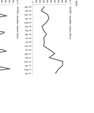
in the Trentino-South Tyrol Italian region. The first was the Museum of Modern and Contemporary
Art whose buildings are placed in the cities of Trento and Rovereto, the two main centres of the
province of Trento. The main building is located in Rovereto, the hometown of the futurist artist
Fortunato Depero, and was designed by the Swiss architect Mario Botta. The museum hosts a
permanent collection where works are displayed on a rotating basis, and a temporary exhibition. It
holds the most important collections in Italy for what concerns different artistic genres of modern
and contemporary art. Figure 1 reports monthly visitors flows. Although the number of observations
is limited there can be deduced an increasing trend in visits.
The second one was the South Tyrol Museum of Archeology (STMA). It is located in Bozen, the
main city of South Tyrol, and hosts the permanent exhibition of Ötzi ‘the iceman’, a mummy from
the Neolithic period of a man living in the region more than 5,000 years ago. Ötzi was found in
September 1991 on Ötztal Alps by two German hikers and at a first sight was thought to be an
unfortunate victim of the mountains. Later scholars discovered that it was one of the oldest
mummies in the world. Due to its good preservation status and the presence of several belongings it
allows scientists to make several investigations about the living conditions of ancient men. The
mummy can be seen by visitors from a window on the so-called ‘Iceman Box’, a refrigerator that
5 series of the number of visitors. What emerges is the more marked seasonal pattern than MART and
the increase in the number of visitors in the last available year.
Due to their geographical location in a valley of a mountain region, both MART and STMA are
potentially addressed to the audience of mountain tourists. Nevertheless, due to its location in
South-Tyrol STMA is accessible by Austrian and German tourists more easily, although the same
transportation lines serve Rovereto (i.e., same highway and railway).
3.2.The questionnaire
The survey was conducted from June to September 2011. A total of 1288 interviews (tourists,
day–visitors, and local residents) were successfully collected from the two museums almost evenly
(46% for MART, 54% in the Ötzi museum). In order to encourage cooperative behaviour
respondents were informed that the research had exclusively scientific aims and that impartiality in
data analysis was guaranteed. Furthermore a pilot survey was carried out to test the questionnaire
before conducting the full survey, in order to avoid biases related to the questionnaire structure and
wording. Interviews were held to visitors exiting the museums after their visit, in selected working
and week-end days of the four months analysed, and during different time periods of the day. Only
one person per travel party was selected. The questionnaires were anonymous and
self-administrated in three languages (Italian, German, and English), though a research team member
was present to respond if questions or doubts emerged. A convenience sampling method was used,
as there were no sufficient information on the characteristics of museums’ visitors in order to apply
a probabilistic design. Of course well known limitations exist in making inference from a
non-probability sampling.
The questionnaire was structured in three sections – see Table 1. The first concerned information
related to the visit to the museum. The second one included trip-related characteristics, whereas the
6
3.3.Profile of visitors
Table 2 compares the profile of visitors to MART and STMA. Three clusters are analysed: total
expenditure, spending in accommodation, and on food and beverage. This distinction will be kept
also in econometric estimates. Total expenditure includes all the items referring to a direct
‘economic trace’ on the visited territory accommodation, food and beverage, shopping in both
museum’s shop and other shops of the city, pharmacy, tour guide services, other expenditures. It
excludes spending on transportation, which usually benefit residents marginally. Expenditure in
accommodation catches the behaviour of those who decided to spend an overnight holiday on the
territory, and as such it includes only tourists. Food and beverage instead is the most
non-discretionary expenditure item besides accommodation that leaves economic traces on the territory,
and unlike accommodation it includes also same-day visitors and residents.
The size of households visiting the museums was bigger for STMA and did not differ
significantly for those who spent in accommodation. This may indicate that same-day visitors
contribute to visit the museum with families of bigger size. The importance of family size is also
confirmed by the higher presence of children and married people in STMA that differed
significantly from MART. A relevant presence of same-day visitors emerges also from comparing
the average length of stay (not reported in Table 1) that equals 1.7 nights for MART and 6.3 for
STMA.
Also the tourists’ origin distribution was significantly heterogeneous. Visitors coming from
abroad, and Germany in particular, are more frequent for STMA, whereas MART appears to attract
more visitors from neighbour regions. Gender differs significantly only for non-overnight visitors,
but the gap between mean ages of visitors is not significant between the two museums.
Variables measuring the economic status provide significant indications about the profile of
7 person or student – the latter feature being significant for non-overnight visitors. The household
annual income is instead higher for those who visited STMA and did not stay overnight.
The earlier descriptive evidence of the spenders’ profiles suggests the presence of two different
typologies of visitor. People with a higher culture and resident in nearby areas visit MART more
frequently. STMA’s audience is instead more attractive for foreigners and families with children.
Often differences between the two museums’ visitors do not appear to be significant for overnight
stayers.
4. Modelling tourist expenditure
4.1.Theoretical framework
Economic theory on tourist consumer behaviour is usually analysed under the classical utility
model. The consumer chooses the quantities of goods and services that maximize her utility, given a
budget constraint and a set of preferences (Papatheodorou, 2006). A basic theoretical model for
studying the factors influencing the level of expenditure can be derived from Downward and
Lumsdon (2000, 2003). If qj|t represents the quantity demanded of the commodity j at time t, pj
is the commodity’s relative price, B
k and Tk are respectively consumer k’s budget constraint and
tastes, demand can be seen as:
qj|t=q p
(
j,Bk,Tk |t)
(1)Considering prices explicitly provides a formulation of demand that is difficult to assess from
8
pjqj
j
!
|t= pq Bk,Tk|t
(
)
. (2)Empirical studies express budgetary limitations and tastes as function of measurable characteristics.
In literature there can be found different classifications of these explanatory variables. The one used
as guideline in this work in order to choose the regressors is the one of Brida and Scuderi (2012),
who distinguish between economic constraints, socio demographic, psychographic and trip-related
variables.
4.2.Econometric model
This study adopts a particular estimation process introduced by Heien and Wessels (1990) in
order to study the determinants of overall expenditure and the two subsets of spending in
accommodation and food and beverage. The choice is driven by the presence of a nontrivial number
of visitors that declared zero expenditure.
Heien and Wessels approach falls into the category of double–hurdle models that were
introduced in Section 2. Also here the consumer is supposed to pass two ‘hurdles’ before
purchasing that are related to ‘selection’ (she decides whether or not to purchase) and ‘outcome’
(she decides how much money to spend for that purchase). Each step corresponds to a distinct
equation, where in Heckman’s (1979) generalized version a Probit model is used for the selection
stage and OLS assesses the factor influencing the outcome. The two models are joined through the
‘inverse Mills Ratio’ (MR), a vector that is added as independent variable to the second stage. MR
is calculated from the estimations of the Probit model (selection stage). Besides being a correction
factor for the censoring, MR’s statistical significance indicates that there have been two stages in
the purchasing decision process. In case MR is not significant the two stages are independent and a
Tobit model can be used. Moreover Heien and Wessells improve Heckman’s (1979) approach with
9 considers in the second stage only those units that declared a positive spending.
4.3.The double–hurdle model: a technical description
Suppose that the willingness to spend of ith visitorfrom a set of n individuals is a latent variable
expressed by y1*i. If X1i is a (n × (1+K)) matrix reporting a column of 1’s corresponding to the
intercept, and K columns each corresponding to an independent variable, the linear relation of
dependence of y1*i from X1i, plus an error term, vi, normally distributed with zero mean and
constant variance, is expressed by
y1*i =X1i!1+vi, (3)
where !1 is a (n × 1) vector. Due to the unobservability of the latent variable there can be defined
an observable dummy variable (y
1i), in which each element is linked to the latent variable by means
the following equation:
y1i=
1 if y1i*
> 0
0 otherwise
! " #
$ #
, (4)
that is y1i equals 1 in case the consumer decides to spend. Given equation (3), relation (4) and the
assumptions made about the error term, we found that the model that described the selection stage is
the Probit model, where the probability that the ith visitor will spend (Maddala, 1983) can be
expressed as:
P y1
(
i=1)
=P X1i!1+vi>0
10
with ! "
( )
being the standard normal cumulative distribution, and zi =
(
X1i!1)
!1. Parameters !1are usually estimated via maximum likelihood and their sign indicates whether a variable increases
or decreases the probability to spend. After estimations of the first stage inverse Mills Ratio (MR) is
computed as:
MRi = !
( )
zi1! "
( )
z1 #$ %& if y1i =1
!
( )
zi "( )
z1 otherwise '( )
* )
, (6)
where !
( )
! is the density function for a standard normal variable. The vector of MR enters asregressor in the second stage and corrects OLS for inconsistencies and biasedness in presence of a
censored variable. The second ‘hurdle’ supposes again that there exist another latent variable, say
y2*, but this time corresponding to the amount the visitor is willing to spend, and another set of
regressors in the matrix X2 of dimension (n × (1+J)), reporting a column of 1’s and a set of J
independent variables. Regressors can differ from the ones of first stage. Also here suppose that for
the ith visitor the following linear relation holds:
y2*i =X2i!2+ui, (7)
with !2 being a vector of (1+J) parameters to be estimated and u
i is the error term normally
distributed with zero mean and constant variance. Since y2* is a latent variable its elements ( ) are
not observable, but it is possible to observe the variable, in which each element ( ) is linked to
the elements of the latent variable as follows:
y2i
*
11 y2i =
y2i *
if y 2i *
>0 and y 1i *
>0 0 otherwise
! " #
$ #
, (8)
which leads to the following linear regression that can be estimated via OLS:
y2*i =X2i!2+"MRi+#i. (9)
In the second-stage regression !
i is a random component with zero mean. The value of !
represents the covariance between v
1 and u1, that is the errors of the two hurdles (Heckman, 1976).
4.4.Selection of regressors
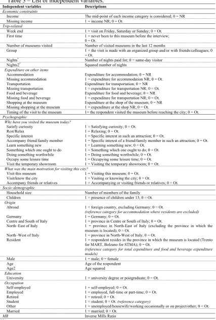
A list of candidate regressors to be included in the model is reported in Table 3. Their
classification is made according to the categories mentioned in Section 4.1, that is economic
constraints, trip-related, psychographic and socio-demographic variables.
Income and expenditure variables are added by a dummy variable assuming the value of 1 when
the respondent does not report the amount. This correction increases the sample size that would
nevertheless be affected by a greater nonresponse rate. Income was surveyed in classes in order to
increase the response rate, but in regressions models it is used as a unique metric regressor where
the centre of each class is the modality. Two other metric variables, that is the number of nights and
age, are added by their squared values in order to test for nonlinear effects.
Due to their high number a selection of regressors is required. In this sense guidelines can
emerge from economic theory. As reported above, indications of theoretical models about the
elements explaining tourist expenditure, and in particular spending behaviour of tourists of cultural
12 limitations and ‘tastes’. An alternative choice could be the selection on the basis of what previous
studies considered in regression analysis. Nevertheless as already stressed no past contributions
study the determinants of spending of tourists visiting museums. Moreover, as the review of
literature by Brida and Scuderi (2012) reports, studies on the determinants of tourist consumption
report a high number of heterogeneous regressors. This implies that indications of literature concern
only the use of regressors that can be classified into categories, such as the four ones we mentioned
above of economic constraints, socio-demographic, trip-related and psychographic variables. Of
course such heterogeneity can be related also to the absence of a robust theoretical framework in
guiding the selection of indicators.
For all these reasons in this paper the choice is oriented by a statistical criterion. In particular
identification is made through a backward stepwise analysis at each ‘hurdle’ of the model. Stepwise
analysis selected those regressors that were significant at a level less than 0.05. Such an approach
has the advantage to operate a choice among the regressors on the basis of an optimality criterion.
The main negative aspect concerns the difficulty in comparing estimated coefficients if different
regressors are selected for each museum. This may affect the objective of comparing the intensity of
coefficients, whereas it allows a qualitative comparison between those elements that emerge as most
significant. Moreover the use of stepwise might sometimes appear as a merely mechanical selection
of regressors, as also stressed by Brida and Scuderi (2012). Nevertheless in a field where no robust
theoretical indications emerge about the selection of regressors this appears as the most reasonable
criterion in order to characterize the spending profile for each museum. Of course future research
would greatly benefit from theoretical works on the economics of cultural visitors.
5. Results
5.1.Total expenditure
13 stepwise at each stage and for each museum. The significance of MR for both models indicates that
the two-stages model is appropriate.
There emerge two distinct profiles of visitors for each museum. Evidence on MART visitors
shows that the probability of spending is positively influenced by the fact that the museum was
visited before going to the city. Variables affecting only the level of expenditure are instead the
number of museums visited in the past twelve months and the high level of education of the visitor,
both influencing it positively; a negative coefficient emerges instead from those who decided to
visit the city only to accompany a friend or a relative. The rest of significant variables affect both
the decision and outcome levels. This concerns those who visited the museum in order to learn
something new, married visitors, and residents outside the province, all being in a positive
relationship with spending. Among non-residents the greatest impact on the level of spending is
given by those who live in foreign countries other than Germany, followed by those living in the
Centre and South of Italy. Instead ‘generalist’ visitors, that is those whose motivation for visiting is
‘doing something worthwhile’, show negative coefficients for both decision and level of spending.
A negative association with those who do not declare their income affects the probability of
spending for STMA visitors, which indicates that those who omitted their wealth status decided to
spend less frequently. The probability of spending is instead higher for weekend visitors and
first-timers. Level of spending is positively influenced by income level and declaring a specific interest
in visiting STM, whereas those who visited temporary showroom and came with a high number of
household members spent a lower amount. Factors influencing both stages are instead the decision
to visit the museum as main motivation to come to Bozen and the origin of visitors, the former
having a negative effect to spending. Similar to MART the spending of visitors is higher for
residents in foreign countries other than Germany and the Centre-South of Italy, meaning that the
higher is the distance the higher is the willingness to spend in general.
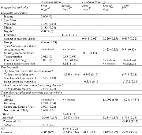
14 The decision of spending in accommodation facilities measures the choice of staying overnight.
As expected income is a significant driver in deciding whether to afford an overnight vacation. Visit
on weekends influences the probability of spending on accommodation facilities. The number of
nights has also a positive influence on the probability of staying in accommodations but the
probability of spending increases at a lower rate as the number of nights raises. Party size has
instead a negative role in deciding whether to stay overnight. Results show also that overnight
stayers visit the museum as one of the attractions of the city, and accordingly think that visiting the
museum is something that one ought to do. The probability to spend on accommodation facilities is
positively related to spending on transportation, food and beverage, and, of course, to living outside
the province, whereas married visitors are likely to decide spending less frequently.
The amount of spending on accommodation appears to be positively associated with first time
visit, spending in transportation, food and beverage, and male respondent. Those who declare that
museum is a chance to learn something new are instead in an inverse relationship with spending, as
well as married respondents. The origin of visitors was not significant in discriminating the decision
of the amount to allocate on this item, whereas it was on deciding whether to spend on overnight
stay. With respect to foreign tourists the ones living in the North-East of Italy (i.e., the nearest area)
is not significant as expected.
The distinction between the two stages of decision and outcome is not significant for expenditure
on food and beverage. As stressed above, the use of Tobit model is here necessary. There emerges a
positive relationship of spending with the number of museums visited, married visitors, spending on
accommodation facilities, and those declaring that the visit is a chance to learn something new. A
negative relationship is instead found with the household size and the generalist opinion that
visiting MART is worthwhile. The only significant category of visitors for what concerns the origin
is the one of those who come from foreign countries other than Germany.
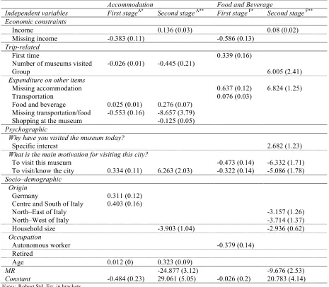
15 Similarly to total expenditure, the decision of spending on both accommodation and food and
beverage for STMA visitors is negatively associated with the omission of income on the
questionnaires. The decision of paying for accommodation is negatively related also with the
number of museums visited. Variables positively affecting the decision of overnight staying are
instead spending on food and beverage, the willingness to visit the city, age, and residence in
Germany and Centre-South of Italy with respect to those living in other foreign countries. The
amount of spending in accommodation facilities is positively associated with income, spending on
food and beverage, willingness to visit the city an age. Negative factors of influence to that amount
of expenditure are the number of museums visited in the last year, shopping at the museum and the
household size.
The probability to spend on food is higher for first time visitors and those who spent on
transportation. Inverse relationship instead emerges from those who are aimed at visiting both the
museum and the city as main activity of the trip and autonomous workers. The amount of spending
is instead positively related to income level, group size and specific interest in visiting STMA. A
negative coefficient instead involves both the museum visit and knowledge of the city as main
motivations for the trip, residence in the North of Italy, household size.
6. Discussion and conclusions
Museums are important attractors for tourists. Nevertheless their role for local communities goes
beyond being a mere attraction for those who take an overnight holiday. The presence of a museum
can be in fact a value added also for residents and for the improvement of the supply of culture in a
territory. Museums visitors are also consumers, and as such they generate positive economic effects
for local economies. Understanding the profile of visitors as spenders can shed light on the
positioning of museums within the tourist supply of a community, and their role in determining
16 different typologies of museums that are located in the same region, and both being potential
attractions for mountain tourists.
The use of opportune econometric modelling was necessary in order to avoid inconsistency and
biasedness of classical OLS estimates. An improved version of double-hurdle modelling as
proposed by Heien and Wessels (1990) was then applied. The analysis considered three different
categories of expenditure. Total spending excluding transportation reflects the ‘economic trace’ that
the tourist leaves on the visited community. Accommodation expenditure characterizes tourists and
their decision of overnight stay. All visitors instead may spend on food and beverage.
Significant differences emerge between the two museums and concur in defining two distinct
profiles of visitors. MART appears as a very relevant attractor for tourism in Rovereto and seems to
exert positive spillover effects to the city. The average visitor has a higher education level than in
STMA and comes with families of smaller size and less frequently in presence of children. For this
museum tourists interested in its cultural value exert a significant and positive effect on total
spending. This is revealed by the positive coefficient of the number of museums visited, of visitors
with higher education, and of those that declared to visit the museum to ‘learn’ something new. A
further support to this interpretation is the negative effect of the ‘generalist’ visiting, that is those
who think that the visit is something worthwhile or come to the museum for accompanying
someone. The subset of those who decided to stay overnight considers MART as one of the
attractions of the territory, but at the same time they are aware that visiting something that one
ought to do. These overnight stayers visit MART mainly on weekends. The intensity of spending on
accommodation is instead negatively related to the opinion of the visiting to the museum as a
moment for learning. Also spending on food and beverage suggests a positive association with the
‘cultural’ tourist. Overall an increasing attention to cultural aspects of exhibitions and activities and
a proper promotion of the cultural value of MART may boost its economic impact. At the same
17 policies should be addressed also to this segment of visitors, although MART effects on the local
economy appear to be mainly due to those that are in search of a ‘cultural’ attraction.
The impact of STMA on the local economy is instead associated to a more ‘generalist’ profile of
visitor. What appears on the whole is that it is perceived more as one of the main attractions that are
part of the tourist supply than for its strict ‘cultural’ value. Moreover the ‘history of the iceman’
seems to attract an audience of families with children more frequently than MART, and that have
also higher income. The pronounced seasonality of visitors’ flows highlight its role of being a
fundamental part of the tourist supply of Bozen, and as such it is influenced by the typical
infra-annual fluctuations similar as to arrivals. This emerges also from the analysis of accommodation
and food and beverage spending, where no particular proxy of ‘cultural’ aspects is related to
spending.
The proposed analysis highlighted how different are the profiles of ‘tourists as spenders’ in two
typologies of museums. Methodologies such as the one proposed can be helpful for both public
policymakers and private investors in order to act on the factors that are likely to boost the
economic impact on territories. One of the limitations of this study is that expenditure patters are
analysed separately for each typology of spending, rather than in an integrated way. Future research
should then consider the consumer’s decision making process in a more complex way, where the
choice to spend a given amount of money for one activity can influence the amount of money that
the visitor is willing to pay for another activity. Interesting suggestions in this sense come from the
work of Zhang et al. (2012) and their quantitative integrated modelling of tourism behaviour.
References
Alegre J., Mateo S., & Pou L. (2010). An analysis of households’ appraisal of their budget
constraints for potential participation in tourism. Tourism Management, 31(1), 45–56.
18 Aristei, D., & Pierani, L. (2008), A double–hurdle approach to modelling tobacco consumption in
Italy, Journal of Applied Economics, 40, 2463–2476.
Bai, J., Wahl, T.I., Lohmar, B.T., & Jikun, H. (2010), Food away from home in Beijing: Effects of
wealth, time and “free” meals, China Economic Review, 21, 432–441.
Barquet, A., Brida, J.G., Osti, L., & Schubert, S. (2011). An analysis of tourists’ expenditure on
winter sports events through the Tobit censorate model. Tourism Economics, 17(6), 1197-1217.
Brida, J. G., Disegna, M., & Osti, L. (2010). The Effect of Authenticity on Tourists’ Expenditure at
Cultural Events (September 10, 2010). Available at SSRN: http://ssrn.com/abstract=1674830
Brida, J.G., & Scuderi, R. (2012). Determinants of Tourist Expenditure: A Review of
Microeconometric Models. Available at SSRN: http://ssrn.com/abstract=2048221
Brida, J.G., Bukstein, D., Garrido, N., & Tealde, E. (2012). Cruise passengers’ expenditure in the
Caribbean port of call of Cartagena de Indias: a cross-section data analysis. Tourism Economics,
18(2), DOI 10.5367/te.2012.0115, forthcoming.
Cragg, J.G. (1971). Some Statistical Models for Limited Dependent Variables with Application to
the Demand for Durable Goods. Econometrica, 39(5), 829–844.
Dolnicar, S., Crouch, G.I., Devinney, T., Huybers, T., Louviere, J.J., & Oppewal, H. (2008).
Tourism and discretionary income allocation. Heterogeneity among households. Tourism
Management, 29(1), 44-52.
Downward, P., & Lumsdon, L. (2000). The demand for day-visits: An analysis of visitor spending.
Tourism Economics, 6(3), 251-261.
Downward, P., & Lumsdon, L. (2003). Beyond the demand for day-visits: An analysis of visitor
spending. Tourism Economics, 9(1), 67-76.
Downward, P., Lumsdon, L., & Weston, R. (2009). Visitor Expenditure: The Case of Cycle
Recreation and Tourism. Journal of Sport & Tourism, 14(1), 25-42.
19 Graburn, N. (1998). A quest for identity. Museum International, 50(3), 13–18.
Heckman, J. J. (1979). Sample selection bias as a specification error. Econometrica, 47(1), 153-161.
Heien, D., & Wessels, C. (1990), Demand system estimation with micro data: a censored regression
approach, Journal of Business & Economic Statistics, 8(3), 356–371.
Hong, G.S., Fan, J.X., Palmer, L., & Bhargava, V. (2005). Leisure Travel Expenditure Patterns by
Family Life Cycle Stages. Journal of Travel & Tourism Marketing, 18(2), 15-30.
Hong, G.S., Kim, S.Y., & Lee, J. (1999). Travel Expenditure Patterns of Elderly Households in the
US. Tourism Recreation Research, 24(1), 43-52.
Hughes, H. L. (2002). Culture and tourism: A framework for further analysis. Managing Leisure,
7(3), 164–175.
Istat (2010). I musei e gli istituti similari non statali. Available at
http://www3.istat.it/dati/catalogo/20110524_00/
Jang, S.C.S., & Ham, S. (2009). A double-hurdle analysis of travel expenditure: Baby boomer
seniors versus older seniors. Tourism Management, 30(3), 372-380.
Jang, S.C.S., Ham, S., & Hong, G.S. (2007). Food-Away-From-Home Expenditure of Senior
Household in the United States: a Double-Hurdle Approach. Journal of Hospitality & Tourism
Research, 31(2), 147-167.
Jones, A.M., & Yen, S.T. (2000), A Box–Cox double–hurdle model, The Manchester School, 68(2),
203–221.
Leones, J., Colby, B., Crandall, K. (1998). Tracking expenditures of the elusive nature tourists of
Southeastern Arizona. Journal of Travel Research, 36(3), 56-64.
Lim, C. (1997). Review of international tourism demand models. Annals of Tourism Research,
20 López–Mosquera, N., & Sánchez, M. (2011), The influence of personal values in the economic– use
valuation of peri–urban green spaces: An application of the means–end chain theory, Tourism
Management, 32, 875–889.
Maddala, G.S. (1983), Limited–Dependent and Qualitative Variables in Econometrics. Cambridge:
Cambridge University Press.
McIntosh, A. J., & C. Prentice, R. (1999). Affirming authenticity: Consuming cultural heritage.
Annals of Tourism Research, 26(3), 589–612.
McKercher, B. (2004). A comparative study of international cultural tourists. Journal of Hospitality
and Tourism Management, 11(2), 95–107
Mehmetoglu, M. (2007). Nature-based tourists: The relationship between their trip expenditures and
activities. Journal of Sustainable Tourism, 15(2), 200-215.
Newman, C.M.H., & Matthews, A. (2001), Infrequency of purchase and double–hurdle models of
Irish households’ meat expenditure, European Review of Agricultural Economics, 28(4), 393–
419.
Nicolau, J.L., & Más, F.J. (2005). Heckit modelling of tourist expenditure: Evidence from Spain.
International Journal of Service Industry Management, 16(3), 271-293.
Papatheodorou, A. (2006). Microfoundations of tourist choice. In L. Dwyer, & P. Forsyth (Eds.),
International handbook on the economics of tourism (pp. 73-88). Cheltenham: Edward Elgar Publishing, Inc.
Saz–Salazar, S., & Rausell–Köster, P. (2008), A Double–Hurdle model of urban green areas
valuation: Dealing with zero responses, Landscape and Urban Planning, 84, 241–251.
Song, H., & Li, G. (2008). Tourism demand modelling and forecasting - a review of recent
research. Tourism Management, 29(2), 203-220.
Thrane, C. (2002). Jazz festival visitors and their expenditures: linking spending patterns to musical
21
Tobin, J. (1958). Estimation of Relationships for Limited Dependent Variables. Econometrica,
26(1), 24-36.
Tufts, S., & Milne, S. (1999). Museums: A supply-side perspective. Annals of Tourism Research,
26(3), 613–631.
Wang Y., & Davidson M.C.G. (2010a). A review of micro-analyses of tourist expenditure. Current
Issues in Tourism, 13(6), 507-524.
Weagley, R.O., & Huh, E. (2004). Leisure Expenditures of Retired and Near-Retired Households.
Journal of Leisure Research, 36(1), 101-127.
Zhang, H., Zhang, J., & Kuwano, M. (n.d.). An integrated model of tourists’ time use and
expenditure behaviour with self-selection based on a fully nested Archimedean copula function.
Tourism Management, http://www.sciencedirect.com/science/article/pii/S0261517712000490 Zheng. B., & Zhang, Y. (2011). Household Expenditures for Leisure Tourism in the USA, 1996 and
22 F IG U RE S F igure 1 – M A RT : m ont hl y vi si tors f low s F igure 2 – S T M A : m ont hl y vi si tors f low s
0
5000 10000 15000 20000 25000 30000 35000 40000 45000
gen-‐10
feb-‐10
mar-‐10
apr-‐10
mag-‐10
giu-‐10
lug-‐10
ago-‐10
set-‐10
ott-‐10
nov-‐10
dic-‐10
gen-‐11
feb-‐11
mar-‐11
apr-‐11
mag-‐11
giu-‐11
0
5000 10000 15000 20000 25000 30000 35000 40000 45000
gen-‐07
apr-‐07
lug-‐07
ott-‐07
gen-‐08
apr-‐08
lug-‐08
ott-‐08
gen-‐09
apr-‐09
lug-‐09
ott-‐09
gen-‐10
apr-‐10
lug-‐10
[image:24.595.293.758.56.435.2]23 TABLES
Table 1 – Structure of the questionnaire
Sections Object Description
I Museum information Repeat visiting; number of museums visited in the last year; push factors*; rating of
factors that describe the visit**; shopping expenditure at the museum; authenticity
perception*.
II Trip information Purpose of the trip; number of nights, expenditure per night and type of
accommodation used by tourists; expenditure per day for different items.
III Interviewees’ profile Some socio-demographic and economic characteristics of interviewees and their
families.
24
Table 2 – Socio-demographic and economic characteristics of the visitors: significance (p-value) of
Chi-square and t-tests.
Variables
Total expenditure Accommodation Food and beverage
MART STMA p
-value MART STMA
p
-value MART STMA
p -value
Household size (mean) 2.05 2.46 ** 2.28 2.49 0.08 1.99 2.38 **
Presence of children (%) ** ** **
Yes 13.88 37.25 19.63 38.15 15.09 35.62
No 86.12 62.75 80.37 61.85 84.91 64.38
Marital status (%) ** ** **
Married 54.94 75.37 56.07 76.88 59.25 73.77
Not Married 45.06 24.63 43.93 23.12 40.75 26.23
Origin of tourist (%) ** ** **
Abroad 3.19 18.74 9.35 17.91 5.28 21.57
Germany 3.70 34.70 14.02 36.90 6.42 33.01
Centre/South of Italy 9.58 14.93 25.23 18.18 12.08 16.34
North–East of Italy 40.34 12.15 26.17 11.82 39.25 13.40
North–West of Italy 13.78 14.35 25.23 15.19 16.98 14.38
Resident
(Bolzano-Trento) 29.41 5.12 --- --- 20.00 1.31
Gender (%) ** 0.54 *
Male 44.05 51.33 50.47 53.77 44.91 53.29
Female 55.95 48.67 49.53 46.23 55.09 46.71
Age (mean) 44.29 44.32 0.97 44.36 44.97 0.63 45.09 44.01 0.31
Level of education (%) ** ** **
University degree 82.58 68.45 85.05 69.11 83.77 68.65
Not university degree 17.42 31.55 14.95 30.89 16.23 31.35
Occupation (%) ** 0.48 **
Autonomous worker 17.76 20.30 21.50 19.95 18.49 17.49
Employed 47.40 59.10 51.40 59.60 45.66 64.03
Other occupation 10.55 8.36 10.28 7.83 12.08 7.92
Retired 12.73 7.46 9.35 8.33 13.21 5.28
Student 11.56 4.78 7.48 4.29 10.57 5.28
Household annual income (%)
** 0.06
**
0 -| 25 000 19.57 9.28 12.15 9.23 13.96 11.11
25 000 -| 50 000 39.13 26.52 41.12 28.43 44.91 28.10
51 000 -| 75 000 11.71 15.36 14.95 19.20 13.96 20.26
> 76 000 7.36 15.36 14.95 17.21 8.30 20.59
Missing income 22.24 33.48 16.82 25.94 18.87 19.93
Notes:
25 Table 3 – List of independent variables.
Independent variables Descriptions Economic constraints
Income The mid-point of each income category is considered; 0 = NR Missing income 1 = income NR; 0 = Ot.
Trip-related
Week end 1 = visit on Friday, Saturday or Sunday; 0 = Ot. First time 1 = never been to this museum before the interview;
0 = Ot.
Number of museums visited Number of visited museums in the last 12 months
Group 1 = the visit is made with an organized group and/or with friends/colleagues; 0 = Ot.
Nights* Number of nights paid for; 0 = same-day visitor
Nights2* Squared number of nights
Expenditure on other items
Accommodation Expenditure for accommodation; 0 = NR Missing accommodation 1 = expenditure for accommodation NR; 0 = Ot. Transportation Expenditure for transportation; 0 = NR Missing transportation 1 = expenditure for transportation NR; 0 = Ot. Food and beverage Expenditure for food and beverage; 0 = NR Missing food and beverage 1 = expenditure for transportation NR; 0 = Ot. Shopping at the museum Expenditure at the shop of the museum; 0 = NR Missing shopping at the museum 1 = expenditure at the shop NR; 0 = Ot.
Timing of the visit to the museum 1= the respondent visited the museum before reaching the city; 0 = Ot. Psychographic
Why have you visited the museum today?
Satisfy curiosity 1 = Satisfying curiosity; 0 = Ot. Rest/Relax 1 = Relaxing; 0 = Ot.
Specific interest 1 = Specific interest in such an attraction; 0 = Ot.
Accompany friend/family member 1 = Specific interest of a friend/family member in such an attraction; 0 = Ot. Learn something new 1 = Learning something new; 0 = Ot.
Something which one ought to do 1 = Something which one ought to do; 0 = Ot. Doing something worthwhile 1 = Doing something worthwhile; 0 = Ot. Occupy some leisure time 1 = Occupying some leisure time; 0 = Ot. Visit the temporary showroom 1 = Visiting the temporary showroom; 0 = Ot. What was the main motivation for visiting this city?
Visit this museum 1 = Visiting this museum; 0 = Ot. Visit/know the city 1 = Visiting or knowing the city; 0 = Ot.
Accompany friends or relatives 1 = Accompanying or visiting friends or relatives; 0 = Ot. Socio–demographic
Household size Number of members of the family Children 1 = presence of children under 13; 0 = Ot. Origin
Abroad 1 = foreign country, excluding Germany; 0 = Ot.
(reference category for accommodation where residents are excluded) Germany 1 = Germany; 0 = Ot.
Centre and South of Italy 1 = province in Centre or South of Italy; 0 = Ot.
North–East of Italy 1 = province in North-East of Italy (excluding the province in which the museum is located); 0 = Ot.
North–West of Italy 1 = province in North-West of Italy; 0 = Ot.
Resident 1 = respondent resides in the province in which the museum is located (Trento for MART, Bolzano for STMA); 0 = Ot.
(reference category for total expenditure and food and beverage expenditure models)
Male 1 = male; 0 = female Age Age of the respondent Age2 Age squared Education
University 1 = university degree or postgraduate; 0 = Ot. Occupation
Self-employed 1 = self-employed; 0 = Ot.
Employed 1 = employed, full-time or part-time; 0 = Ot. Retired 1 = retired; 0 = Ot.
Student 1 = student; 0 = Ot. (reference category)
Other 1 = unemployed/housewife/working occasionally or on project/other; 0 = Ot. Married 1 = married; 0 = Ot.
MR Inverse Mills Ratio Notes
*
26 Table 4 – Determinants of total expenditure per capita per day (excluding transportation), significant regressors (p < 0.05). Standard errors are reported in parenthesis.
MART STMA
Independent variables First stage*M Second stage**M First stage*S Second stage**S Economic constraints
Income 0.231 (0.04)
Missing income -0.659 (0.12)
Trip-related
Weekend 0.292 (0.12)
First time 0.380 (0.15)
Number of museums visited 0.842 (0.24)
Timing of the visit to the museum 0.391 (0.17)
Psychographic
Why have you visited the museum today?
Specific interest 4.981 (2.52)
Learn something new 0.428 (0.14) 11.060 (3.05)
Doing something worthwhile -0.338 (0.15) -10.777 (2.66)
Visit the temporary showroom -5.683 (2.85)
What is the main motivation for visiting this city?
Visit this museum -0.274 (0.12) -8.074 (2.56)
Accompany friends or relatives -6.871 (2.77)
Socio–demographic
Origin
Abroad 1.473 (0.39) 62.475 (9.86) 2.088 (0.38) 62.910 (6.42)
Germany 1.328 (0.36) 35.368 (5.79) 1.947 (0.36) 52.828 (5.37)
Centre and South of Italy 1.091 (0.23) 40.240 (4.52) 2.172 (0.38) 58.986 (6.81)
North–East of Italy 0.338 (0.14) 19.583 (2.43) 1.679 (0.38) 51.237 (5.88)
North–West of Italy 0.799 (0.19) 35.702 (4.65) 1.780 (0.37) 54.081 (5.73)
University 5.565 (2.38)
Married 0.352 (0.11) 6.816 (2.96)
Household size -8.362 (1.44)
MR -38.895 (4.41) -39.576 (2.36)
Constant -0.802 (0.17) 16.445 (2.82) -1.244 (0.35) 27.254 (5.7)
Notes: Robust Std. Err. in brackets. *M
Number of obs = 590; Wald chi2(9) = 82.14; Prob > chi2 = 0; Log pseudolikelihood = -357.5794; McKelvey and Zavoina's R2 = 0.223; **M
Number of obs = 590; F(12,577) = 16.87; Prob > F = 0; Adjusted R2 = 0.271
*S
Number of obs = 650; Wald chi2(9) = 88.05; Prob > chi2 = 0; Log pseudolikelihood = -322.29457; McKelvey and Zavoina's R2 = 0.248;
**S
27 Table 5 – MART: determinants of expenditure on accommodation and food and beverage, per capita per day, significant regressors (p < 0.05). Standard errors are reported in parenthesis.
Accommodation Food and Beverage
Independent variables First stageA*
Second stage A**
First stage F*
Second stage F**
Tobit F*** Economic constraints
Income 0.006 (0)
Trip-related
Week end 0.355 (0.15)
Nights 0.183 (0.04)
Nights2 -0.003 (0)
First time 4.037 (1.31)
Number of museums visited 0.044 (0.02) 0.326 (0.15) 0.617 (0.22)
Group -0.486 (0.19)
Expenditure on other items
Accommodation Not included Not included 0.423 (0.12) 0.54 (0.12)
Missing accommodation 0.81 (0.15)
Transportation 0.012 (0) 0.13 (0.03)
Food and beverage 0.031 (0) 0.613 (0.15) Not included Not included
Missing transportation/food 3.547 (1.6) Not included Not included Psychographic
Why have you visited the museum today?
To learn something new -4.339 (1.64) 0.342 (0.15) 6.748 (3.31)
Something which one ought to do 0.525 (0.19)
Doing something worthwhile -0.356 (0.15) -5.872 (2.86)
What is the main motivation for visiting this city?
To visit/know the city 0.534 (0.23)
Socio–demographic and economic characteristics
Origin
Abroad Not included Not included 13.992 (6.6) 16.281 (7.37)
Germany 1.278 (0.34)
Centre and South of Italy 0.973 (0.22)
North–West of Italy 0.698 (0.2)
Male 3.234 (1.3)
Married -0.546 (0.17) -2.987 (1.48) 3.234 (1.17) 8.736 (2.23)
Household size -3.488 (1.17)
Children 0.502 (0.2)
MR 14.642 (2.21)
Constant -2.05 (0.22) -3.645 (1.14) -0.31 (0.1) 2.037 (0.92) -5.79 (3.73)
Notes: Robust Std. Err. in brackets. A*
Number of obs = 589; Wald chi2(14) = 163.88; Prob > chi2 = 0; Log pseudolikelihood = -167.30885; McKelvey and Zavoina's R2 = 0.630; A**
Number of obs = 589; F(8,580) = 14.17; Prob > F = 0; Adjusted R2 = 0.407 F*
Number of obs = 504; Wald chi2(4) = 44.61; Prob > chi2 = 0; Log pseudolikelihood = - 324.02271; McKelvey and Zavoina's R2 = 0.151; F**
Number of obs = 504; F(9,499) = 10.39; Prob > F = 0; Adjusted R2 = 0.321; F***
[image:29.595.55.519.114.554.2]28 Table 6 – STMA: determinants of expenditure on accommodation and food and beverage, per capita per day, significant regressors (p < 0.05). Standard errors are reported in parenthesis.
Accommodation Food and Beverage
Independent variables First stageA* Second stage A** First stage F* Second stage F** Economic constraints
Income 0.136 (0.03) 0.08 (0.02)
Missing income -0.383 (0.11) -0.586 (0.13)
Trip-related
First time 0.339 (0.16)
Number of museums visited -0.026 (0.01) -0.445 (0.21)
Group 6.005 (2.41)
Expenditure on other items
Missing accommodation 0.637 (0.12) 6.824 (1.25)
Transportation 0.076 (0.03)
Food and beverage 0.025 (0.01) 0.276 (0.07)
Missing transportation/food -0.553 (0.16) -8.657 (3.79)
Shopping at the museum -0.125 (0.05)
Psychographic
Why have you visited the museum today?
Specific interest 2.682 (1.23)
What is the main motivation for visiting this city?
To visit this museum -0.473 (0.14) -6.332 (1.71)
To visit/know the city 0.334 (0.11) 6.263 (2.03) -0.322 (0.14) -5.086 (1.78)
Socio–demographic Origin
Germany 0.311 (0.12)
Centre and South of Italy 0.403 (0.16)
North–East of Italy -3.157 (1.26)
North–West of Italy -3.714 (1.37)
Household size -3.903 (1.04) -2.936 (0.62)
Occupation
Autonomous worker -0.379 (0.14)
Retired
Age 0.012 (0) 0.323 (0.09)
MR -24.877 (3.12) -9.676 (2.53)
Constant -0.484 (0.23) 29.061 (5.05) -0.026 (0.2) 20.783 (4.14)
Notes: Robust Std. Err. in brackets. A*
Number of obs = 647; Wald chi2(8) = 90.54; Prob > chi2 = 0; Log pseudolikelihood = - 380.04211; McKelvey and Zavoina's R2 = 0.282; A**
Number of obs = 647; F(9,637) = 20.99; Prob > F = 0; Adjusted R2 = 0.238 F*
Number of obs = 555; Wald chi2(7) = 77.44; Prob > chi2 = 0; Log pseudolikelihood = - 328.88707; McKelvey and Zavoina's R2 = 0.300; F**
[image:30.595.55.520.114.520.2]