Contents lists available atScienceDirect
International
Journal
of
Approximate
Reasoning
www.elsevier.com/locate/ijar
Particle
MCMC
algorithms
and
architectures
for
accelerating
inference
in
state-space
models
Grigorios Mingas
a,
Leonardo Bottolo
b,
Christos-Savvas Bouganis
a,
∗
aDepartmentofElectricalandElectronicEngineering,ImperialCollegeLondon,London,SW72AZ,UK bDepartmentofMedicalGenetics,UniversityofCambridge,Cambridge,CB20QQ,UK
a
r
t
i
c
l
e
i
n
f
o
a
b
s
t
r
a
c
t
Articlehistory:
Received15May2016
Receivedinrevisedform23September 2016
Accepted24October2016 Availableonlinexxxx
Keywords:
MarkovChainMonteCarlo Particlefilter
Fieldprogrammablegatearray Bayesianinference
Hardwareacceleration
ParticleMarkovChainMonteCarlo(pMCMC)isastochasticalgorithmdesignedtogenerate samples froma probability distribution, when the density of the distributiondoes not admit aclosed form expression. pMCMC is most commonly used to sample from the Bayesian posterior distribution in State-Space Models (SSMs), a class of probabilistic models used in numerous scientific applications. Nevertheless, this task is prohibitive whendealingwithcomplexSSMswithmassivedata,duetothehighcomputationalcost of pMCMC and its poor performance when the posterior exhibits multi-modality. This paper aimstoaddressbothissuesby:1)Proposing anovelpMCMC algorithm(denoted ppMCMC), whichusesmultiple Markov chains (insteadofthe one used bypMCMC) to improve sampling efficiency for multi-modal posteriors, 2) Introducingcustom, parallel hardware architectures, which are tailored for pMCMC and ppMCMC. The architectures are implemented on Field Programmable Gate Arrays (FPGAs), a type of hardware accelerator with massive parallelization capabilities. The new algorithm and the two FPGA architectures are evaluated using a large-scale case study from genetics. Results indicatethatppMCMCachieves1.96xhighersamplingefficiencythanpMCMCwhenusing sequentialCPUimplementations.TheFPGAarchitectureofpMCMCis12.1xand10.1xfaster thanstate-of-the-art, parallelCPU and GPU implementationsof pMCMC and upto 53x moreenergyefficient;theFPGAarchitectureofppMCMCincreasesthesespeedupsto34.9x and 41.8x respectivelyand is 173xmorepower efficient,bringingpreviouslyintractable SSM-baseddataanalyseswithinreach.
©2016TheAuthors.PublishedbyElsevierInc.ThisisanopenaccessarticleundertheCC BYlicense(http://creativecommons.org/licenses/by/4.0/).
1. Introduction
MarkovChainMonteCarlo(MCMC)algorithmsareoneofthefundamentaltoolsusedtosamplefromcomplexprobability distributions.TheyarepopularforsamplingfromposteriordistributionsinBayesianinference,whicharetypicallycomplex andhavelargedimensions. Thesesamplesare usedto estimateintegrals,whichare neededinorderto inferparameters, make predictions,performmodel comparison, etc.[1].This processis calledMonteCarlointegration.[2]and[1]contain examplesofhowMCMCsamplesareusedinvariousapplications.
MostMCMC algorithms [1]are based on theassumption that the densityof the sampleddistribution (denoted p
(θ )
, whereθ
isthesampledvariable)canbeevaluatedpointwiseuptomultiplicativeconstant.Nevertheless,therearemodeling*
Correspondingauthor.E-mailaddresses:[email protected](G. Mingas),[email protected](L. Bottolo).
http://dx.doi.org/10.1016/j.ijar.2016.10.011
0888-613X/©2016TheAuthors.PublishedbyElsevierInc.ThisisanopenaccessarticleundertheCCBYlicense (http://creativecommons.org/licenses/by/4.0/).
scenarios in Bayesian statistics where it is not possible to evaluate the probability density because it doesnot admit a closedformexpression.TheseincludeinferenceforStateSpacemodels(SSMs)[3],stochastickineticmodels[4],undirected graphicalmodels[5].Thesecasesareoftencalled“analyticallyintractable”intheMCMCliterature.
The pseudo-marginalMCMC sampler introduced by [6]marked a major breakthroughin this field:It showed that if an unbiased estimatorofthe sampleddensityisused insideMCMC (instead oftheclosed formexpression), thesampler still convergestothecorrectdistribution.Alargebodyofworkhasexploitedthisremarkablepropertyduringthelastfive years toconstructnewMCMCalgorithms.ThemostwidelyappliedamongthemisParticle MCMC(pMCMC)[3],whichis designedforinferenceonSSMswithunknownparameters.
SSMs withunknown parameters is a widely usedclass ofBayesian models. Theyare applicable toproblems wherea sequence ofunknown (hidden)statesneeds tobeinferredfromknownobservationsandtherelationshipsbetweenstates andobservationshaveunknownparameterswhichalsoneedtobeinferred.Asimpleexampleistargettracking,whereboth the positionofthetracked objectandthenoisein sensormeasurementsare unknown andneedtobe inferredfromthe measurements.ThistypeofSSMinferenceisknowntoleadtoanalyticallyintractabledensities[3].pMCMCusesaParticle Filter(PF)[7]tounbiasedlyestimatethe density(which isanaturalchoiceforSSMs).Therefore,itiscapable ofinferring theSSMposterior.
pMCMChasextendedtheapplicabilityofSSMstoareaslikeecology[8],communicationnetworks[9],systemsbiology
[10]andmarinebiogeochemistry[11].Nevertheless,thecomputationalcostofestimatingthedensityusingaPFisO
(
T·
P)
(where T isthe numberofhiddenSSM statesand P isthe numberofparticles ofthe PF) [12].Moreover, each pMCMC iteration requires a separate PF run andtypically thousands ofiterations are needed. This means that usingpMCMC for large SSMsiscomputationally prohibitive.When conventionalCentralProcessingUnits (CPUs)are employed theruntimes can reach months oryears [11,10]. The work presented herewas initially motivatedby such a complex problem:SSMs in genetics,where T,which corresponds toDNA bases,can reachmillions (see[13] andSection 6).This situationforces practitionerstocollectfewerMCMCsamples(whichleadstoincreasedvariance)oruseasimplermodeland/orfewerdata. Inaddition tothiscomputational burden,theissueofmulti-modalityintheposterior(i.e.theexistenceofmanyareas ofhighprobability)isentirelyunaddressedinpMCMCliterature.Nevertheless,multi-modalitycanappearingenetics appli-cations(seeSection6and[13]).Insuchcases,pMCMCexplorestheposteriordensityslowly,acommonproblemformany MCMCmethodswhichisknownasslowmixing.
Inordertohandletheabovelimitations,thisworkfollowstwomaindirections.First,itproposesanewalgorithm,which is abletosample frommulti-modaldistributions moreefficientlythanpMCMC.Second, itleveragesthepower ofparallel hardwareacceleration.Morespecifically,itusesaclassofhardwaredevicescalledFieldProgrammableGateArrays(FPGAs), which offermassiveparallelresourcesandhavethedistinctivecharacteristicthat theirhardware architecturecan befully customizedaccordingtotherequirementsoftheimplementedalgorithm.Evenmorecrucially,thisworkcombinestheabove twoapproachestofurtherincreaseperformance;algorithmicandhardwaredesignaredonejointlysothatinformationabout thenatureoftheunderlyinghardwarecanbeexploitedwhendesigningthealgorithmandviceversa.Thecontributionsof thisworkaresummarizedbelow:
1. AnewMCMCalgorithm,denotedPopulation-based Particle MCMC–ppMCMC,whichis anextension ofpMCMCand whichusesapopulationofchainsinsteadofthesinglechainusedbypMCMC.ppMCMCimprovesmixingfordensities whichare bothanalyticallyintractableandmulti-modal(Section4).AjustificationofwhyppMCMCworks, i.e.whyit convergestothedesiredposteriordistribution,isalsoprovided.
2. AnovelparallelhardwarearchitectureforpMCMC,implementedonanFPGA,whichexploitstheparallelisminsidethe PFtoimprovesamplingthroughput(Section5.2).
3. Anovelparallelhardware architectureforppMCMC,alsoimplementedonanFPGA,whichpipelinesthecomputations ofthemultipleppMCMCchainstoincreasetheutilizationofthePFdatapathinsidetheFPGA(Section5.3).
ThenewalgorithmandthetwoFPGAsamplersareappliedtoalarge-scaleinferenceproblemingenetics–anSSMmodel ofDNAmethylationwithunknownparameters(Section6).Thismodelcanleadtouni-modalormulti-modalposteriors.In theformercase,theFPGApMCMCsampleriscomparedtooptimized,state-of-the-artCPUandGPUimplementationsandit isfoundtobe6.4x–14.9xand3.8x–30.8xfasterrespectively.Inthelattercase,thetrade-offbetweenthenumberofchains and thenumber ofPF particles inppMCMC is explored tomaximize performance. Whencomparing sequential software implementationsofthealgorithms,ppMCMCis1.96xfasterthanpMCMC.WhencomparingtheFPGAimplementations,the FPGAppMCMCisupto3.24xfasterthantheFPGApMCMCsamplerandupto34.9xand41.8xfasterthantheCPUpMCMC andGPUpMCMCsamplersrespectively.
Thepaperisorganizedasfollows.Section2providesthenecessarybackgroundonBayesianinference,SSMsandpMCMC, aswellasashortintroductiononFPGAs,whileSection3givesanoverviewofprevious literature.Section4introducesthe newppMCMC algorithmandSection 5describestheproposedFPGAarchitectures.Section 6containsa descriptionofthe case studies used to evaluate the method, followed by Section 7 which presents the results of the evaluation. Finally, Section8concludesthepaper.
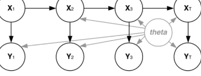
Fig. 1.Hidden states, observations and unknown parameters of SSM.
2. Background
2.1. Bayesianinference
Bayesianinferenceisasimpleframework,whichconsistsininferringtheprobabilitydistributionoftheunknown quan-titiesofaprobabilisticmodelgiventheknowndata.Thisisdonebycombining:1)Informationabouttheunknownsbefore anydataareavailable,i.e.thepriordistributionoftheunknowns,2)Informationabouttheunknownsprovidedbythedata, i.e.thelikelihoodoftheunknowns. Theinferreddistributioniscalledtheposteriordistributionoftheunknownsgiventhe data.Practitionersaretypicallyinterestedinevaluatingorestimatingexpectations(integrals)overthisposterior.Theform oftheseintegralsdependsontheapplicationandisoutsidethescopeofthispaper(formoreinformationsee[2]and[1]).
2.2. State-spacemodelswithunknownparameters
SSMswithunknown parametersareaclassofBayesianmodels,whereahiddensequenceofstateswhichevolvesover time emitsasequence ofobservations,whilethe functionsthatdefine therelationships betweenstatesandobservations haveunknownparameters.Moreformally,letXt
∈
R
nX bearandomvariablerepresentingthestateoftheSSMattimestep t∈ {
1,
...,
T}
,wherenX∈
N
.LetYk∈
R
nY be another randomvariablerepresenting theobservationvector attime stept,where nY
∈
N
. Timesteps here can representtime, space, etc., depending onthe application. AnSSM is definedby the followingsetofequations:X1
∼
e(X
1) (1)Xt
∼
f(X
t|
Xt−1,θ),
t>
1 (2)Yt
∼
g(Y
t|
Xt,θ
),
t>
0 (3)Here,e
(
X1)
istheinitialprobability density, f(
Xt|
Xt−1,
θ
)
istheprobability densityofmovingto thecurrentstate giventhepreviousstate(transitiondensity)andg
(
Yt|
Xt,
θ
)
istheprobabilitydensityofobservingthecurrentobservationgiventhe current state (observationdensity). The two densities also depend on a set of unknown parameters,
θ
∈
R
nθ with nθ∈
N
.Usually,differentpartsoftheθ
vector areusedin(2)and(3)butherethewholevectorappearsinbothdensitiesforsimplicity.Symbol“
∼
”meansdistributedaccordingto.Fig. 1depictsthestructureofanSSM.From the standpoint ofBayesian inference, the unknown quantities that need to be inferred are 1) the hidden state sequence X1:T and 2) the unknown parameters
θ
. It is assumed that the random variablerepresenting the observationvectorisknown,i.e.Y1:T
=
y1:T,wherey1:T isaknownvector(alsocalledthedata).ThereforethegoalofSSMinferenceistoinferthefollowingjointposterior:
p
(X
1:T,θ
|
Y1:T=
y1:T)
=
p(X
1:T,
θ
|
y1:T)
∝
ρ
(θ)
π
(X
1:T|
θ) λ(y
1:T|
X1:T,θ
)
=
ρ
(θ
)
e(X
1) T t=2f(X
t|
Xt−1,θ)
tT=1g(y
t|
Xt,
θ)
(4)Here,
ρ
(
θ
)
is the Bayesian prior density ofthe parameterθ
,π
(
X1:T|
θ
)
is the Bayesian prior densityof the states andλ(
y1:T|
X1:T,
θ
)
isthelikelihoodofthedata(observations)giventheunknowns.Theright-most partofthesecond lineoftheequationiseasilyderivedfromthedensitiesofSection2.2(see[7]fordetails).
2.3. pMCMC:jointstateandparameterestimationinSSMs
pMCMC(Algorithm 1)solvestheSSMinferenceproblemstochastically,i.e.bydrawingsamplesfromthejointposteriorof equation(4).Inotherwords,pMCMCgeneratesasequenceofN jointsamples
(
X1:T,
θ
)
1:N,whicharedistributedaccordingto p
(
X1:T,
θ
|
y1:T)
.Ateach loop iterationin line9,pMCMCperforms threesteps:1) Itproposesa candidatesample
θ
∗ fortheunknown parameter basedonthe previous sampleθ
, usinga simpleprobability densityq(
·
| ·
)
(line10). 2) Itcalls a PFalgorithm (which willbeexaminedlater)toachieve twothings:First,togenerateasetof P samplesfromp(
X1:T|
y1:T,
θ
∗)
.One ofthesesamplesisselectedrandomlyinline12andserves astheproposed statesequencesample X∗1:T.Second,toproduce anunbiasedestimateofthequantityl
(
y1:T|
θ
∗)
,whichisthelikelihoodofthedata,giventheSSMparameters.Theestimateisdenotedby
˜
l(
y1:T|
θ
∗)
anditisnecessaryforthefollowingstepofthealgorithm.ThePFrunisthemostcomputationallyintensivepartofpMCMC.3)Itacceptsthejointcandidatesample
(
X∗1:T,
θ
∗)
withprobabilitymin(
1,
a)
wheretheacceptance ratioais:a
=
ρ(θ∗)˜l(y1:T|θ∗)q(θ|θ∗) ρ(θ)˜l(y1:T|θ)q(θ∗|θ)(5)
Otherwisetheprevioussampleisreplicated(lines13–20).Thefirstiteration(lines2–7)onlyperformsstep2toinitializethe sampler.TheinputsofpMCMCarethenumberofMCMCiterations(N),theinitialparametersample(
θ
init)andthenumber ofparticles ofthePF(P).The algorithmreturnsthehistoryofsamples Sample[
1:
N]
andposteriors P osterior[
1:
N]
after all N iterationshavebeencompleted.Algorithm1ParticleMCMC. 1:procedurepMCMC(P,N,
θ
init) 2:Firstiteration(i=1): 3: ˜l(y1:T|θinit),X
11::PT ←PF(P,θinit)//PFrun 4: Sampleindexp∈ {1,...,P},setX
init1:T=Xp 1:T 5: Sample[1]=(Xinit1:T,θ
init
) //saveinitialsample 6: P osterior[1]=ρ(θinit)l˜(y1:T|θinit)//saveposterior 7: θ=θinit//temporaryvariable
8:Remainingiterations: 9: fori=2,...,Ndo
10: θ∗∼q(θ∗|θ) //proposenewcandidatesample 11: ˜l(y1:T|θ∗),
X
11::PT
←PF(P,θ∗)//PFrun 12: Sampleindexp∈ {1,...,P},set
X
∗1:T=X1p:T13: Accept(X∗1:T,θ∗)withprobabilitymin(1,a) 14: ifacceptedthen
15: //savecandidatesampleandposterior 16: Sample[i]=(X∗1:T,θ∗)
17: P osterior[i]=ρ(θ∗)˜l(y1:T|θ∗) 18: θ=θ∗//temporaryvariable 19: else
20: //replicateprevioussampleandposterior 21: Sample[i]=Sample[i−1]
22: P osterior[i]=P osterior[i−1]
23:return(Sample[1:N], P osterior[1:N])
The criticalcontributionof[3]istheproof that,aslongasthelikelihoodestimatesinthenumeratoranddenominator of theratio(5)are unbiased,the algorithmconvergesto the“correct” distribution,i.e.theposterior p
(
X1:T,
θ
|
y1:T)
. ThelikelihoodestimatesprovidedbythePFareunbiased,sopMCMCsamplesfromthe“correct”posterior.Moreover,thisistrue regardlessofthevarianceofthePFestimate.
Asmentionedabove,runningaPFisnecessaryateachiterationofpMCMCinordertogenerateacandidatesampleofthe SSMstatesandan unbiasedestimateoftheSSMlikelihood.PFsareapowerfulclassofmethodsusedforstate estimation inSSMs.ABootstrapPF(Algorithm 2)isusedhere,asitisthemostpopularPFvariant.
The inputsofAlgorithm 2arethenumberofparticles (P) andthecandidate
θ
∗ (generatedinthepreviousstepofthe pMCMCalgorithm).ThePFusesthesetofP particlestoestimateeachstateinthesequenceX1:T.Ateveryiteration(line 8),itpropagatesparticlestothenextSSMtimestepusing:1) Sampling(lines13–15)wherethetransitiondensity(2)isused to sample particles for thenext state, 2) Weighting (lines 16–17) wherethe observationdensity(3) is usedto calculate weightsforallparticles.Theweightquantifiesthequalityofaparticleasanestimateofthenextstate,3)Resampling(lines 9–12),whereanewparticlesetisgenerated,inwhichparticleswithlargeweightsarereplicatedmanytimesandparticles withlowweightsarediscarded (equivalenttomultinomialsampling).ResamplingiscriticalforthestabilityofthePF(see
[7]).
After all T time steps have finished, the ensemble of all particle sets X11::PT is available. Also, the algorithm uses the computedweights toproduceanestimate ofthelikelihood(line19).Thisestimateisunbiased[7].Theoutputs ofthePF areusedinsidepMCMC.Specifically,arandomparticlesequenceischosenfromtheensembleX1:P
1:T (line12ofAlgorithm 1)
andthelikelihoodestimateisusedintheacceptancestep,asdescribedabove.
The main tuningparameter ofpMCMCis thenumberof particles(P). Withlarger P,each pMCMC iterationbecomes moretime-consumingbutthevarianceofthelikelihoodestimatedecreases.ThelatterleadstofasterpMCMCmixing[14], i.e.fasterexplorationoftheposterior,sincepMCMCmovesclosertoanexactMCMCalgorithm.Therefore,thereisatradeoff betweentheruntimeofthePFandthemixingofpMCMC.
Thechoiceoftheproposaldistributionq
(
·|·
)
isalsoatuningparameterofthealgorithm.Inpractice,aGaussianproposal isoftenusedanditsvarianceisadjustedtomaximize mixing.Thisistheapproachfollowedinthisarticle;amultivariateGaussianproposalisusedanditscovariancematrixistunedforeachexaminedSSMposterior(theexactcovariancematrices canbefoundinSection6.1).Finally,likeinallMCMCalgorithms,itisusualtodiscardaninitialchunkoftheN samplesas burn-in,inordertomakesurethesamplerhasconvergedtothetargetdistribution.Thispracticeisfollowedinthisarticle, aswillbedetailedinSection6.1.
Algorithm2BootstrapParticleFilter.
1:procedurePF(P,
θ
∗) 2:Initialstate(t=1): 3: fork=1,...,Pdo4: SampleparticlefrominitialdensityX˜k 1∼e(X1) 5: fork=1,...,Pdo
6: CalculateinitialweightW1k←g(y1| ˜Xk1,θ∗) 7:Remainingstates:
8: fort=2,...,T do
9: fork=1,...,Pdo
10: Sampleancestorindexakfrom{1
,...,P}with 11: probabilitiesproportionalto{W1
t−1,...,W P t−1} 12: andsetresampledparticle
X
kt−1← ˜X ak t−1 13: fork=1,...,Pdo
14: Sampleparticlefromtransitiondensity 15: X˜k t∼f(Xt|Xkt−1,θ∗) 16: fork=1,...,Pdo 17: CalculateweightWk t←g(yt| ˜Xkt,θ∗) 18:Likelihoodestimate: 19: ˜l(y1:T|θ∗)←tT=1 1 P P k=1Wkt 20:return(˜l(y1:T|θ∗),
X
11::TP= {X11:P,...,X1T:P})2.4. FieldProgrammableGateArrays
FPGAsareapowerfulanduniqueclassofdigitalhardware devices,whicharetypicallyusedasacceleratorsfor compu-tationally intensivealgorithms. FPGAs fundamentally differfromother hardware devices suchasCentral ProcessingUnits (CPUs)or Graphics Processing Units (GPUs).While CPUs andGPUs havefixed hardware architecturesdefined beforethe chipismanufactured, FPGAsconsist ofare-programmable “fabric”upon whichanycustom hardware architecturecan be mapped[15].AsFig. 2 shows,the FPGAfabricconsist ofanarray ofprogrammable logicblocksandahierarchyof inter-connectswhichallowtheblockstobewiredtogether.Eachblockcanimplementasimplebooleanfunction.Byconnecting theblockstogether anydigitalcircuitcanbe implemented.Moreover,modernFPGAsareequippedwithdedicatedunitsto performcommonarithmeticoperations,aswellasseveralon-chipmemoryblocks.
FPGAsallowthedesignertotailorthehardwaretothespecificcharacteristicsoftheapplication.Thenumberand gran-ularity ofparallel processingelements, the kinds ofarithmetic operators embedded in theseelements, the amount and architectureofcachememoriesandthearithmeticprecisionofcomputationsareallcustomizable.Thus FPGAscanexploit non-obvious and/or limitedparallelism, maximize pipelining efficiencyand adaptthe memory architecture to the access
pattern ofthe algorithm. Forexample, whilea GPU architecture hasa pre-defined amount ofon-chipmemory per pro-cessing core, an FPGA can allocatea custom amountof on-chipmemoryto each “processingelement” or evenallow all elements toaccessallthememory,depending ontherequirementsofthetargetedalgorithm.Moreover,theprogramming of thefabriccan bedone asmanytimesasdesiredandevenduring runtimeand/or partially.Allthisflexibility canlead to significantlyhigherperformance[15] andlowerpowerconsumption [16]comparedtofixed-architecturedevices(CPUs, GPUs).Nevertheless,FPGAdesignrequiresspecializedprogrammingskillsandlongerdevelopmenttimesthanCPUandGPU coding,despitetherecentemergenceofvarioushighleveltools[17].Inaddition,CPUsandGPUsremaincompetitiveforthe typesofproblemstheyaredesignedfor;sequential/conditionalcodeandSingle-Instruction-Multiple-Data(SIMD)algorithms respectively.
Thisisthe mainreasonwhichhasledhardwaremanufacturers todevelop devicesthatcombinetraditionalCPUswith acustomFPGAfabriconthesamechip[18].Thesedevicescombinethebenefitsofbothworlds;theyallowthesequential and non-criticalpart ofthe targetedalgorithm (including librariesthat might be hard to migrateto an FPGA) tobe run on theCPU,while thecustom fabricisresponsible fortheparallel, computationallyintensivepart.Different architectures can be loaded onthe fabric depending onthe algorithm.It isexpected that thesehybridchips willplay an increasingly important roleinthe datacenterandhighperformance computingmarkets,wherethe demandforhighthroughputand low poweris strong.AlgorithmslikeMCMCandPFare commonlyusedinthesecomputingenvironments,since they are fundamentaltoolsfornumerouslarge-scalescientificapplications.
3. Relatedwork
ThefirstworkonparallelaccelerationofpMCMCusingGPUswaspublishedin2012[19].Thesampleandweightstepsof thePFwereparallelizedandasystematicresamplingalgorithmwasimplementedusingaparallelprefix-sumtechnique.No detailsontheGPUdeviceandthespeedupsoversoftwarewerepresentedandthecasestudiesweresmallSSMs(T
=
100). Thereforetheefficiencyoftheimplementationcannotbeevaluated.Moreover,thelimitednumberofstatesandparticlesis notrepresentativeofreal,large-scaleproblemswherehardwareaccelerationisneeded.A more recentwork [10] proposed an automated tool (LibBi) forSSM inference on CPUsand GPUs whichsupported pMCMC.LibBi providesadomain-specific languageforSSMsandaparallelprocessingback-end(combiningMPI, OpenMP, SSE andCUDA). Nevertheless,the language is inflexible in terms of the definable transition/observation densities; some populardensitiesandseveralcommontypesofcomputationsarenotsupported.Some ofthesedisadvantagescanbe mit-igatedby thefactthatthetool isopenlyavailableandcanbemodified. [10]alsocontains limitedresultsonapplyingthe framework to a Lorenz ’96SSMwith T
=
40 and P=
8192.The evaluationshowedthat using the framework ona CPU withOpenMPandSSEoptimizationswas5xfasterthanrunningsequentialC++code;thecombinedCPU/GPUversion(with CUDA)providedanextra4xspeedup.TheworkpresentedhereisthefirsttouseFPGAstoaccelerate pMCMC,takingadvantageoftheuniquefeaturesofthe platform (e.g. custom pipelining)to accelerate sampling. It isalso the firstto usea modified, parallelized version of the Residual SystematicResampling algorithm inside the PF (first introduced in [20]). Finally, thiswork isthe first to apply pMCMCtolargeSSMs,whereT andP scaletomanythousands.
In the algorithmic level,[21] and [14] haveproposed ways to optimize P based onthe tradeoffbetweenPF runtime andpMCMCmixing,whichwasmentionedabove.Dependingonassumptions,theyrecommendthat P shouldbechosenso thatthevarianceofthelikelihoodestimateisbetween1.0and3.2,inordertomaximizepMCMC’smixingpersecond(the “exploration”ofthestatespacethatpMCMCachievesperunitofcomputingtime).Nevertheless,thefollowingissuesremain unaddressed:1)WhenoptimizingthevalueofP,both[21]and[14]assumethatthePF’sruntimegrowsproportionatelyto
P;thisisnottruewhenusingparallelimplementationofthePFalgorithm.2)TheuseofmultipleMCMCchainstoimprove mixinghasnotbeenexamined,althoughitisclearthatpMCMCcanmixveryslowlyformulti-modalposteriors,evenwith large P.
This worktackles thefirst issueby takingintoaccount theperformance ofparallel PFimplementations (eitherin the FPGAorintheCPU/GPU)whenoptimizingthevalueofP.Inordertoaddressthesecondissue,anovelpMCMCsampler (de-notedppMCMC)isintroduced,alongwithan accompanyingFPGAarchitecture.ppMCMCimprovesmixingformulti-modal posteriors byutilizingmultipleMCMCchainsinsteadoftheoneusedinpMCMC.The“correctness” ofthenewalgorithm, i.e.thefactthatitsamplesfromthecorrectSSMposterior,isalsojustified.Moreover,incontrastto[21]and[14],where P
istheonlyoptimizedparameter,thepresentworkjointlyoptimizes P andM(thenumberofMCMCchainsinppMCMC)in ordertofindthecombinationthatmaximizedmixingpersecond.
Finally, this is the first use of pMCMC and FPGAs for methylation analysis (see the case study of Section 6). So far, pMCMC was considered intractable for such problems and approximatemethods were used [22], leading to bias in the resultingestimates.
4. ppMCMC:anewMCMCalgorithm
4.1. Summary
This section presents a novel MCMCalgorithm, which extendspMCMC by adding auxiliary MCMCchains in order to improve mixinginscenarios wheretheSSM posterior(4)is multi-modal,such asthe onepresented inSection 6.
Multi-modalityistheexistenceofmultipleareasofhighprobabilityintheposterior[23].StandardpMCMCfacesthewell-known issueofslowmixingwhensamplingfromsuchposteriors.Thisissueiscommoninmanysingle-chainMCMCmethods.The samplertendsto“getstuck”inoneofthemodesoftheposteriorandrarelymanagestomovetoanothermode[23].
ThenewalgorithmiscalledPopulation-based ParticleMCMC(ppMCMC)anditisacombinationoftwoexistingMCMC methods(Population-basedMCMC[23]andpMCMC).Thepseudo-codeofppMCMCisgiveninAlgorithm 3.Itmakesuseofa populationofMpMCMCchains.Ateachiteration(loopinline 10),ppMCMCperformstwokindsofoperationsforallchains. The first is the updateoperation (loop in line12), during which the next MCMC sample of each chain is generated, usingthe samethreesteps described forpMCMC: 1)Propose acandidateunknown parameter sample
θ
∗ (line 13) using densityqj(
·
| ·
)
forchain j∈ {
1,
...,
M}
.LikeinpMCMC,multivariateGaussianproposaldistributionsare usedinppMCMC.The covariance matrix of these distributions can be tuned. 2) Run a PF to propose a candidate state sequence sample
X∗1:T andan estimate ofthe likelihood (lines 14–15). 3) Accept thejoint candidatewith probability min
(
1,
aj)
for chain j∈ {
1,
...,
M}
. Otherwise repeat the previous sample (lines 16–24). The difference compared to pMCMC is the use of a differentacceptance ratiofor each chain(step 3). This leads each chain tosample froma differentdistribution. Chain 1 samplesfromthe“correct”posterior(4).Theotherchainssamplefrom“smoothed”versionsof(4)andtheirmixingisfaster thanthemixingofthefirstchain,aswillbeexplainedinSection 4.2.Onlythesamplesofthefirstchainarekept.Thesecondoperation withineachiterationofppMCMCistheexchangeoperation(loopinline26),whichwasnotused inpMCMC.Duringthisoperation, pairsofneighboring chains (e.g.
(
1,
2)
,(
3,
4)
,etc.)exchange their MCMCsampleswith probabilitymin(
1,
eq)
(forpair(
q,
q+
1),
q∈ {
1,
...,
M−
1}
).Sample exchangeshelp thealgorithmmixfasterbecausetheypushsamplesfromtheauxiliarychainstothefirstchain,helpingittoescapefromlocalmodes.Thisisexplainedinmore detailbelow.
Algorithm3Population-basedParticleMCMC.
1:procedureppMCMC(P,N,M,
θ
init 1:M,T emp1:M) 2:Firstiteration(i=1): 3: forj=1,...,Mdo 4: ˜l(y1:T|θinitj ), X11::PT ←PF(P,θinitj )//PFrun 5: Sampleindexp∈ {1,...,P}andsetX
init1:T←X p 1:T 6: Sample[j][1]←(Xinit 1:T,θ init j )//savesample 7: P osterior[j][1]←ρ(θinit j ) ˜ l(y1:T|θinitj ) 1 T emp j
8: θj←θinitj //temporaryvariable(chain j) 9:Remainingiterations:
10: fori=2,...,Ndo
11: Chainupdates:
12: forj=1,...,Mdo
13: θ∗∼qj(θ∗|θj)//proposenew
θ
(chain j) 14: ˜ l(y1:T|θ∗),X
11::PT ←PF(P,θ∗)//PFrun 15: Sampleindexp∈ {1,...,P}andsetX
∗1:T=X1p:T16: Acceptcandidatesample(X∗1:T,θ∗) 17: withprobabilitymin(1,aj) 18: ifacceptedthen
19: Sample[j][i]=(X∗1:T,θ∗)//savesample 20: P osterior[j][i]=ρ(θ∗)˜l(y1:T|θ∗)
1
T emp j
21: θj=θ∗//temporaryvariable(chain j) 22: else 23: Sample[j][i]=Sample[j][i−1] 24: P osterior[j][i]=P osterior[j][i−1] 25: Chainexchanges: 26: for(q,r)=(1,2),(3,4),. . .OR(q,r)=(2,3),(4,5),. . .do 27: Sample[q][i]↔Sample[r][i] 28: P osterior[q][i]↔P osterior[r][i] 29: θq↔θr
30: withprobabilitymin1,eq 31:return(Sample[1][1:N],P osterior[1][1:N])
4.2. Updateandexchangeoperations 4.2.1. Updates
Duringtheupdateoperationforchain j
∈ {
1,
...,
M}
,thefollowingacceptanceratioisused:aj
=
ρ(θ ∗)˜l(y 1:T|θ∗) 1 T emp j q j(θj|θ∗) ρ(θj)˜l(y1:T|θj) 1 T emp j q j(θ∗|θj),
j∈ {
1, ...,
M}
(6)where T empjisthetemperatureofchain j and1
=
T emp1<
T emp2< ...
<
T empM<
∞
.Therefore,onlychain j=
1 usestheacceptanceratioofpMCMC(givenin(5))andthussamplesfromthe“correct”SSMposterior.Theremaining(auxiliary) chains (j
∈ {
2,
...
M}
)useatempered acceptanceratio,i.e.the estimatedlikelihoodinthenumeratorandthedenominator israisedtothepowerof T emp1j forchain j.Thisleadstheauxiliarychainstosample fromsomesetof“smoothed”(closer
to uniform) versions ofthe “correct” SSMposterior. Chains withsmoother densities mix faster, since itis easier forthe samplertojumpbetweenmodeswhenthemodesaresmoothed.
Althoughapplyingatemperaturetothelikelihoodisawell-knowntechniqueinpopulation-basedmethods,inthecaseof ppMCMCitisnotclearwhatthetargetdistributionofeachtemperedchainis.Thetermp
(θ )
p˜
(
y1:T|
θ )
1
T emp jp
(
X1:T|
y1:T,
θ )
(which contains the likelihood estimate)is used in the acceptance ratio of chain j but this doesnot lead the chain to convergetotheposteriorp
(θ )
p(
y1:T|
θ )
1
T emp jp
(
X1:T|
y1:T,
θ )
,asonewouldintuitivelyexpectaftercomparingtothepMCMCacceptanceratioin(5).
According to the theory presented in [6], a pMCMC chain converges to a target distribution provided that unbiased estimates ofthe distribution’sdensity areused inthe numeratoranddenominator of theacceptance ratio.Nevertheless, the term p
(θ )
p˜
(
y1:T|
θ )
1
T emp jp
(
X1:T|
y1:T,
θ )
is notan unbiased estimatorof p(θ )
p(
y1:T|
θ )
1T emp jp
(
X1:T|
y1:T,
θ )
: Runninga PFonthe givenSSM producesan unbiasedestimate p
˜
(
y1:T|
θ )
of thelikelihood(i.e.E
˜
p
(
y1:T|
θ )
=
p(
y1:T|
θ )
).How-ever, applying thetemperature afterthe likelihood estimate is generated (i.e.finding p
˜
(
y1:T|
θ )
1
T emp j) doesnot maintain
unbiasedness withrespecttothe “correct”temperedlikelihood (i.e. p
(
y1:T|
θ )
1
T emp j). Inmoredetail,becausethe function
x
→
x1
T emp j isconcaveforT empj
≥
1,applyingJensen’sinequality[24]leadstothefollowing:E
p˜
(y1
:T|
θ )
1 T emp j≤
E
p˜
(y1
:T|
θ )
1 T emp j=
p(y1
:T|
θ )
1 T emp j (7)Thisis trueforall ppMCMCchains sincealltemperaturesare greaterorequalto one.Equalityholdsonlyfor T empj
=
1.Therefore, unbiasedestimatesofthe“correct”tempered likelihooddensities p
(
y1:T|
θ )
1
T emp j (andthustherespective
pos-teriordensities)canbeacquiredonlywhenT empj
=
1 (i.e.onlyinthecaseofthefirstchain).Nevertheless,thisdoesnotmean that the tempered chains donot convergeto any target distribution. Infact, chain j convergesto the distribution whose density is unbiasedlyestimated by p
(θ )
˜
p(
y1:T|
θ )
1 T emp jp
(
X1:T
|
y1:T,
θ )
. The densities of thesedistribution can bewrittenas: pj
(X
1:T, θ
|
y1:T)
=
p(θ )
E
˜
p(y
1:T|
θ )
1 T emp jp(X
1:T|
y1:T, θ ),
j∈ {
1, ...,
M}
(8)These are theactual target densities of the M chains ofthe ppMCMC algorithm. Only for the first chainthe density is equaltothe“correct”temperedposterior(withT emp1
=
1)andalsotothe“correct”SSMposterior,i.e. pj(
X1:T,
θ
|
y1:T)
=
p(
X1:T,
θ
|
y1:T)
.Thekeypoint hereisthat itisnotnecessaryfortheauxiliary chainstosample fromthesetof“correct”temperedposteriors,sincetheirsamplesarenotkept.Onlythesamplesofthefirstchainarekeptbecausetheyaretheones distributedaccordingtothedesired,“correct”SSMposterior.Theauxiliarychainsareonlyemployedtohelpthefirstchain mix faster;they need toexplore thedistribution spacequickly(andthereforetheir target distributions needtobe closer touniform)andoccasionallyfeedthefirstchainwithsamplesthroughexchangemoves.Thesesampleshelpthefirstchain escapefromlocalmodes,aswillbeexplainshortly.Itisthereforeenoughfortheauxiliarychainstosamplefromsomeset oftemperedversionsoftheSSMposterior(andnotnecessarilyfromthe“correct”setoftemperedposteriors).Thedensities inequation(8)providethistemperingeffectandthereforefulfill theirpurpose,i.e.theymovefastinthedistributionspace andhelpthefirstchainmixfasterthroughexchangemoves.
Infact,theterm“correct”isonlyusedhereforreasonsofclarity;thereisnoreasontobelievethatthe“correct”densities
p
(
y1:T|
θ )
1
T emp j arethebestcandidatesforuseinauxiliarychains(withrespecttothemixinggainstheyoffer).Ontheother
hand,thisdoesnot meanthatanydensitywouldserveasagoodauxiliarydensity,e.g. uniformauxiliary densitieswould not help the mixingof the first chain because they are not concentrated around the true modes. In other words, some
smoothingmustbeappliedtothetruedensitiesbuttheformoftheoptimalauxiliarydensitiesisnotknown.
Regardingthechoiceofthetemperaturevalues,theyoftenfollowageometricoradditiveprogressioninMCMCliterature, i.e. Ti+1
Ti=constant orTi+1
−
Ti=
constant,althoughother choiceshavealsobeenconsidered[25].Intheevaluationsectionofthisarticle,ppMCMCtemperaturesfollowanadditiveprogression.TheexacttemperaturevaluesaregiveninSection6.
4.2.2. Exchanges
Inordertoexploitthetemperingprocessdescribedabovetoimprovemixing,ppMCMCmakesuseofsampleexchanges, which attempt to swap samples between chains at each iteration. Exchange moves are attempted between chain pairs
(
1,
2),
(
3,
4),
. . .
orchainpairs(
2,
3),
(
4,
5),
. . .
(neighboring chains)inarotatingorder.Asmentionedabove, theexchange movespushMCMCsamplesfromthehigh-temperaturechains,whichareclosertotheuniformdistribution,tothe lower-temperature chains, which are closerto the “correct” target distribution. Eventually samplesreach the first chain whichsamplesfromthe“correctdistribution”andhelpitescapefromlocalmodes.Theexchangeacceptanceratiobetweenchains
(
q,
r)
is: eq=
˜l(y1:T|θr) 1 T empq ˜l(y 1:T|θq) 1 T empr ˜l(y1:T|θq) 1 T empq ˜l(y 1:T|θr) 1 T empr (9)whereq
∈ {
1,
...,
M−
1}
,r=
q+
1 and(
Xq1:T,
θ
q)
and(
Xr1:T
,
θ
r)
arethecurrentsamplesofchainsqandrrespectively.IthastobenotedthattheaboveratiorequiresnoadditionalPFruns(allthevaluesarealreadyknownfromtheprecedingupdate steps).
Itisimportanttojustifywhytheaboveexchangemovefulfills therequirementsofthetheoryofpMCMC[6]withregards to maintainingthecorrecttarget distributions ofthe twochains. Theexchange step isequivalent toa Metropolisupdate where the updated state is the jointstate ofboth chains (withindexes q and r). According to [6],a Metropolis update maintainsthetargetdistributionaslongasthenumeratoranddenominatoroftheacceptanceratioareunbiasedestimates ofthetargetdensity.Inthecaseoftheexchangestep(andfocusingonlyonthenumeratorforsimplicity),thismeansthat the product p
(θ
r)
p˜
(
y1:T|
θ
r)
1 T empq p(
Xr 1:T|
y1:T,
θ
r)
p(θ
q)
p˜
(
y1:T|
θ
q)
1 T empr p(
Xq 1:T|
y1:T,
θ
q)
(denoted by U) hasto be anunbiasedestimateoftheproductofthetargetdensitiesofthetwochains(which weregiveninequation(8)).Itiseasyto show that thisisthe case.Since p
(θ
r)
, p(
Xr1:T|
y1:T,
θ
r)
, p(θ
q)
and p(
Xq1:T|
y1:T,
θ
q)
are all zero-varianceestimators,thefollowingistrue: E
[
U] =
E
[
p(θ
r)
p˜
(y
1:T|
θ
r)
1 T empq p(X
r 1:T|
y1:T, θ
r)
p(θ
q)
˜
p(y
1:T|
θ
q)
1 T empr p(X
q 1:T|
y1:T, θ
q)
] =
p(θ
r)
p(X
r1:T|
y1:T, θ
r)
p(θ
q)
p(X
q1:T|
y1:T, θ
q)
E
˜
p(y
1:T|
θ
r)
1 T empq p˜
(y
1:T|
θ
q)
1 T empr (10)Moreover,it isknownthat p
˜
(
y1:T|
θ
r)
1
T empq and p
˜
(
y 1:T|
θ
q)
1
T empr are independentestimators(sincetheyare generatedby
two independent PFs, each assigned to its own MCMC chain). Therefore, their product is equal to the product of their expectations.Combiningthiswithequation(10),itisclearthat:
E
[
U] =
p(θ
r)
p(X
r 1:T|
y1:T, θ
r)
p(θ
q)
p(X
q 1:T|
y1:T, θ
q)
E
p˜
(y1
:T|
θ
r)
1 T empqE
p˜
(y1
:T|
θ
q)
1 T empr=
pq(X1
:T, θ
r|
y1:T)
pr(X1
:T, θ
q|
y1:T)
(11)Thelast lineoftheequation istruedueto equation(8)andproves thattheproduct U isan unbiasedestimateofthe of theproductofthetargetdensitiesofthetwochains.
5. FPGAarchitecturesforpMCMCandppMCMC
ThissectionpresentsnovelFPGAarchitecturesforpMCMCandppMCMC,whichexploittheinherentparallelismofeach algorithm.
5.1. Parallelisminthealgorithms
In pMCMC, the available parallelism is O
(
P)
, since all particles inside the PF can be processed inparallel (although resampling requires communication between parallel processes). The N iterations of pMCMC are strictly sequential. In ppMCMC,the availableparallelism increasesto O(
M·
P)
duetotheexistence of M MCMCchainswhich canbe updated independently(althoughexchangesrequireinter-chaincommunication).Theindependenceoftheupdateoperationscanbe exploitedtopipelinecomputationsinthePFdatapath.5.2. pMCMCarchitecture
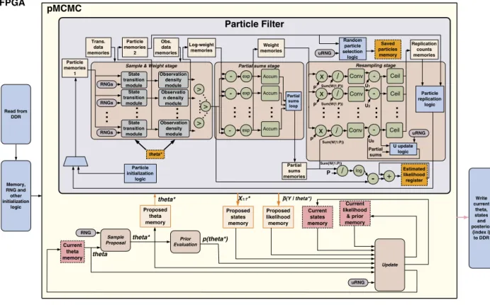
The pMCMCarchitectureis illustratedin Fig. 3.ThepMCMC blockwithin thearchitecture comprises allthe necessary parts of an MCMC sampler plus a PF block. The PF block comprises three stages: Sample & Weight, Partial sums and Resampling(groupedinadifferentwaycomparedtothedescriptionofSection2.3forimplementationreasons).Theoutput MCMCsamplesarestoredinexternal(off-chip)memory,whichisnotshowninthefigure(moredetailsbelow).
AteverypMCMCiteration(i
∈ {
1,
...,
N}
),thecurrent(latest)θ
sampleisreadfromtheCurrentthetamemoryandsentto theSampleProposalblock,whichsamplesfromq(
θ
∗|
θ
)
.Thecandidateθ
∗ iswrittentotheProposedthetamemoryand for-wardedtothePF.Thelatterreturnstheestimatedlikelihood˜
l(
y1:T|
θ
∗)
andarandomlyselectedstatesampleX1∗:T=
Xp1:T;thesearewrittentotherespectivememories.ThePriorEvaluationblockcomputestheprior
ρ
(
θ
∗)
.TheUpdateblockaccepts orrejects(
X∗1:T,
θ
∗)
basedon(5),usingseveralinputvalues.Iftheupdateissuccessful,thecandidatesample andthe pro-posedlikelihoodandpriorvaluesarewrittentotherespectivecurrentmemories(equivalentto Sample[
i]
and P osterior[
i]
Fig. 3.FPGAarchitecturefor pMCMC.Theorangememoryblocksareinputs/outputsofthePF.ThepinkmemoryblocksareoutputsofpMCMC. (For interpretationofthereferencestocolorinthisfigurelegend,thereaderisreferredtothewebversionofthisarticle.)
each iteration,thecontentsofthecurrentmemoriesaresent totheoff-chipmemory.Theabovesteps arerepeatedforall pMCMCloopiterations.
PFblock:ThisblockisactivatedonceperpMCMCiteration.Thesample,weightandresamplingoperationsarerepeated
T times,onceforeverytimestep,withtheorderofoperationschangedcomparedtoAlgorithm 2.Eachstephastoprocess all P particles(loopsinlines9,13and16).Computationsforeachparticleareindependent,thereforetheyareparallelized andpipelined. Thearchitecture’sparallelism (number ofparallel modules)isthe sameforall stepsandis denotedby B. Eachparallel moduleprocesses PB particles.Eachmemorythatfeedsthemodules ispartitionedintoB sub-memoriesand eachsub-memoryisassignedtoonemodule.
The transitionand weight operations are implemented inside the Sample&Weight stage of the architecture. At each stept,particlesX1t−:P1 arereadfromtheParticlememoriesandfedtotheB Statetransitionblock.Thesesamplefrom(2)using
θ
∗astheparameter.TheoutputiswrittentoParticlememories2andpassedtotheBparallelobservationdensitymodulesto computethelog-weightslog(
W1:Pt
)
using(3)(workingwithlog-weightshelpsavoidnumericalissues).Again,thecandidateθ
∗isusedastheparameterin(3).Thelog-weightsarewrittentotheLog-weightmemoriesandpassedtoacomparatortree tofindthemaximumlog-weight.Thefollowingtwostagesofthearchitectureimplementresampling(equivalenttolines9–12ofAlgorithm 2),usingthe Residual Systematic Resampling(RSR)algorithm[20].RSRrequiresthepartialsumsofweightsforeachparallelprocessing module,i.e.modulel
∈ {
1,
...,
B}
requiresthesum(l−1)P B
k=1 W
k
t.RSRoutputsthereplicationcountsofallparticles(r1:P),i.e.
thenumberoftimeseachparticleisreplicated.
In the PartialSumsstage: 1) The maximum log-weight isused for renormalizationto avoid numerical issues,2) Log-weightsareexponentiatedtofindtheweightsand3) Bparallelaccumulatorsproducethesumsofweightsofeachmodule
l
PB
k=(l−1)P B+1
Wtk
,
l∈ {
1,
...
B}
.Thesearethen usedtogeneratethepartialsumsandthesumofall weights.Inthe Resam-plingstage,theRSRarchitecture proposedin[20]isused. B pipelineddatapathscomputethereplicationcountsandwrite them to therespective memory. Detailscan be found in[20]. Afterall countsare stored, they are read sequentiallyand particlekiscopiedfromParticlememories2toParticlememories1 rk times.Theuseoftwomemoriesisnecessarytoavoidoverwriting particlesbefore their replicationcountsare examined. Theprocess cannot be parallelizedby replicatingeach bunch of PB particlesindependently,sincethetotalnumberofreplicationsofabunchmightexceedthememorypartition assignedtoit(1Bthofthetotalmemory).Forinstance,ifP
=
10 and B=
2,eachparallelblockwouldprocess5replication counts/particles andhavea particlememoryoflength5to itsdisposal.Ifparticlek=
1 hasareplication countof6,thisFig. 4.FPGA architecture for ppMCMC.
meansthat thefirst parallelblock doesnothaveenough memoryspaceto replicatetheparticleandneeds toaccessthe secondmemoryblock.Thereplicationprocesswasnotexaminedin[20].
Inparalleltoresampling,themeanofthecurrentweightsiscomputed(usingthepartialsums),itslogarithmisfound, therenormalization(mentionedabove)isinvertedandtheresultisfedto anaccumulator(below theResamplingstage in
Fig. 3).AfterthePFstageshavebeenrepeated T times,thisaccumulatoroutputs thefinalestimate ofthelog-likelihood:
log
(
˜
l(
y1:T|
θ
∗)
=
T
t=1log(
1PP
k=1Wtk
)
.ThisiswrittentotheProposedlikelihoodmemory.Also,afterT timestepstheSaved particlesmemorycontains arandomlyselectedsetofparticles,i.e.theproposedstate X∗1:T,whichiscopiedtotheProposed statesmemory.Allmemories haveconstant sizes, basedonuser-defined parameters (maximum states Tmax,maximumparticles Pmax, nθ,nX andny).
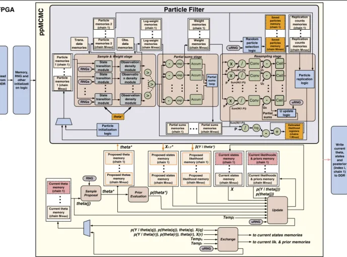
5.3. ppMCMCarchitecture
The ppMCMC architecture is based on the pMCMC architecture but differs in two ways: 1) It permits many chains (M)to beprocessedconcurrently bythe PFdatapath,2)It performsexchange movesbetweenchains.The Proposedtheta,
Proposedstates, Proposedlikelihood, Currenttheta, Currentstates, Currentlikelihood and Priormemories are replicated Mmax
times(maximumnumberofchains,setbytheuser).Thisway,eachchainhasitsseparatememoryandcanbeupdatedand exchangedwithoutinterferingwiththeotherchains.
TheppMCMCarchitectureisshowninFig. 4.TheSampleproposalblockproposes
θ
∗samplesforall Mchainsandwrites themtotherespectivememories.Whenitfinishes,thePFcomputesthelikelihoodsandstatesamplesforallchainsusing coarse-grainpipelining(seenext paragraph).OnlyonePFblockisinstantiated(asinpMCMC);allchainsareprocessedby thisoneblock.ThisisfollowedbytheUpdateandExchangeblockswhichuseequations(6)and(9)toperformtherespective operations.TheUpdateblockneedsanextrainputcomparedtopMCMC–thechaintemperatureT empj.TheExchangeblockattemptsswapsbetweenpairsofchainsassoonasbothchainshavebeenupdatedbytheUpdateblock(i.e.itdoesnotwait forallchaintobeupdatedaswasthecaseinAlgorithm 3).
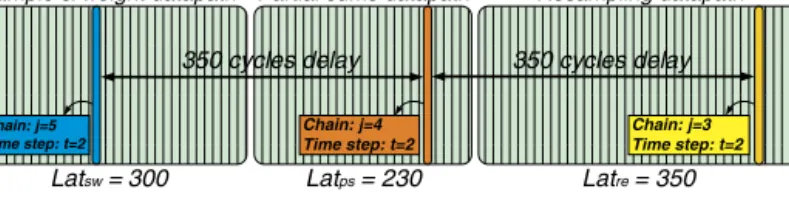
Fig. 5.Coarse-grainpipelininginppMCMCarchitecture:Resamplinghasthelargestlatency,thusanewchainisfedtothePFdatapatheveryLatre=350 cycles.Chains j=3:5 areinthedatapath,allofthemattimestept=2.Chain j=4 willstartResamplingonecycleafterchainj=3 finishesResampling.
Coarse-grainpipelininginthePF:ThePFblockisthesameasinpMCMC(i.e.asingleblock)butexploitstheindependence of ppMCMCchains to increase datapathutilization. Running the PFfora single chain requirestraversing thedatapath T
times,witheach traversalcomprisingthe Sample&Weight, PartialsumsandResampling stages.Eachtraversalhasto wait untiltheprevious onefinishes;also,each stagecanstartonlyafterthepreviousstage finishes.Thismeansthat,withone chain (asinthecaseofpMCMC), onlyoneofthe stagesisutilizedatagivenmoment.Let Latsw, Latps andLatre be the latenciesofthethreestagesforonetimestep(forall P particles).Thenthetotaldatapathlatencyis Latsw
+
Latps+
Latre.Withoutpipelining,thetotallatencyforM chains(withT timestepseach)isM
·
T·
(
Latsw+
Latps+
Latre)
.The ppMCMC architecture coarsely pipelines chain computations,exploiting the fact that the PF run of chain j does not need to wait forthe PF run ofchain j
−
1 tofinish. Multipletasks are processed inthe PFat the sametime, with the following order: First, time step t=
1 of chain j=
1 is processed,followed by time step t=
1 of chain j=
2, etc. When all the firsttime steps have finished,the second time steps (t=
2) are fed to thePF forall chains andso on.By thischangeintheorderofoperations,theavailable parallelismisexposed.Pipelining iscoarse-grain,sincenoPFstage is shared bytwo chainsatthe sametime(toavoidsignificant controloverheads);each chainwaits fortheprevious oneto finisha stagebeforeentering thesamestage.Using thistechnique (Fig. 5), anewchaincanbe fedtothedatapatheverymax
(
Latsw,
Latps,
Latre)
cycles,bringingthetotallatencyforMchains(T timestepseach)toM·
T·
max(
Latsw,
Latps,
Latre))
.Resourceoverheads:Inordertorunmany“virtual”PFsonthesinglePFhardwareblocksimultaneously,multiplememories areusedforallPF-accessedvariables.TheppMCMCarchitectureusesMmax Particle,Log-weight,Weight,Savedparticles, Repli-cationcountsandPartialsumsmemories (eachpartitionedinto B blocksasinpMCMC). TheExchangeblockisanadditional overheadbuttakesfewresources(seeSection7).
5.4. Performancemodels
ThelatencyoftheSample&weightstageinpMCMCis:
Latsw
=
C1+
ceil(
log(
B))
·
Latcomp+
PB (12)whereC1isthe(applicationdependent)latencyoftheparallelmodules,thesecondtermisduetothecomparatortreeand
PB
isthelatencyforpassing P particlesthroughtheparallelmodules.ThelatencyofthePartialsumsstageis:Latps
=
C2+
PB·
Latadd+
B·
Latadd (13)where C2 isthe latencyof theparallel modules,
BP·
Latadd is thelatency forpassing P particles throughthe datapath(Latadd istheadderlatency)andB
·
Latadd isthelatencyofthepartialsumsloop.ThelatencyoftheResamplingstageis:Latre
=
C3+
PB+
P·
Latrep (14)whereC3isthelatencyoftheparallelmodules,
PBisthelatencyforpassingP particlesthroughthedatapathandP·
Latrepistheparticlereplicationlatency(Latrepisthemeanreplicationcount).OnePFruninpMCMCcosts:
Latp f_pMC MC
=
PB+
T·
(
Latsw+
Latps+
Latre)
(15)where
PBisduetoparticleinitialization.InppMCMC,processingonetimestepforallchainscosts:
Latts_ppMC MC
=
C4+
M·
max(
Latsw,
Latps,
Latre)
+
Latsw
+
Latps+
Latre−
max(
Latsw,
Latps,
Latre)
(16)
where C4 isduetominorcomputationsbeforeeachtime step.Thelatencyofprocessingall T time stepsofall M chains
is:
Latp f_ppmcmc
=
M·
BP+
T·
Latts_ppmcmc (17)6. Casestudy:SSMsforDNAmethylationprofiling
Inordertoevaluatetheproposedalgorithmandarchitecturesoftheprevious sections,alarge-scalesyntheticSSMcase studywhichfocusesonDNAmethylationisused.Thiscasestudyisdesignedtodemonstratethebenefitsofthealgorithmic andhardwarearchitecturenoveltiesproposedinthisarticle,usingarealistic,demandingapplication.
MethylationisabiochemicalprocesswhichhappensinspecificpositionsoftheDNAandisassociatedwithanumberof diseases.Thepositionswheremethylationhappenscannotbedetecteddirectly.Methylationanalysisconsistsindiscovering these “hidden” positions by applying a process called sodium bisulfate treatment to the DNA bases, several times. The treatmentis essentiallyatest formethylation,whose outputiseitherasuccessfulora faileddetection. Nevertheless,the test can belargely unreliableandnoisy in manycasesandfurther analysisis neededtosuccessfully detectmethylation. Methylation analysiscan be applied to single-tissue ofmulti-tissue DNA. The latter caseoccurs when processing mixed tissue,e.g.whole-bloodsamples.
MethylationdatacanbesimulatedusingSSMmodels;thehiddenmethylatedstatescan berepresentedbythehidden statesoftheSSMandSSMinferencecanbeusedtoestimatethembasedonknownobservations(i.e.thebisulfatetreatment testresults).SSMshavetheadvantagethattheycanrepresentdependenciesbetweenneighboring statesusingthetransition density;thisisimportantformethylationmodeling,sincethemethylationstateofaDNAbasedependsonthestateofthe neighboring bases.
Here,twosyntheticDNAmethylationdatasetsaresimulatedusingSSMs:1) Asingle-tissuedataset,2)Amulti-tissue dataset.First,therealmethylationproblemsettingwillbepresented,followedbyadescriptionofhowthisismappedtoan SSM.Ineachcase,theDNAsequenceisassumedtohavealengthofT bases,wherebaset
∈ {
1,
...,
T}
hasprobability pt of beingmethylated.Thegoalistoestimatetheseprobabilitiesusingtheresultsofmethylationtestson4biologicalreplicatesk
∈ {
1,
...,
4}
(i.e.individualswithidenticalDNAsequences).Atbaset andforreplicatek,asodiumbisulfatetreatmenttest isappliednkt times.Outofthesetests, ykt aresuccessful. ThephysicalpositionofDNAbaset isδ
t.The physicalpositionis neededbecause typically some gaps exist betweenbases inreal data sets. The goalof theanalysis is todiscover the probability pt thatpositiont ismethylated,forallt.Inthiscasestudy,T rangesupto16384.
TheabovesettingismappedtoanSSMasfollows:
•
The logit-probabilitythat thebaset ismethylated, i.e.logit(
pt)
isthe hiddenstate Xt ofthe SSM.Therefore,X1:T=
logit(
p1:T)
.•
Thenumberofsuccessfultestsatbaset oftheDNAsequence,forallfourreplicates(y1:4,t)istheobservationyt oftheSSM,i.e.y1:T
=
y1:4,t.Thenumberoftestsatpositiont(n1:4,t)isalsopartoftheobservations.The transition,prior andobservationdensities oftheSSMare constructedasfollowsto simulatetherealsetting: The transitiondensity(2) forthe single-tissueDNAcase modelsthe fact that theprobabilities of methylationare dependent betweensubsequentDNAbases:
Xt
∼
Normal(X
t−1,τ
2t
),
t>
1 (18)where
τ
2t isthetransitionvariance.Thisisafunction ofacommonvariance
σ
12 andtheDNAphysicalposition(δ
t):τ
t2=
σ
21
|
δ
t−
δ
t−1|
.Thevarianceσ
12representstheamountofdependencebetweenthemethylationstatesofsubsequentbases.The transitiondensity inthe multi-tissue DNAcase (with two tissues)is similar butin thiscase a mixture of Gaus-sian densitiesis usedinsteadof oneGaussian. Thismixturerepresents thefact thattwo tissues withdifferentinter-base dependenceexistintheDNAsample:
Xt
∼
2c=1wc
·
Normal(X
t−1, ψtc2)
,
t>
1 (19)where wc
=
0.
5 is the weight of the mixture componentwith indexc∈ {
1,
2}
andψ
tc2=
σ
2c
|
δ
t−
δ
t−1|
. Here,σ
c2 isthetransitionvarianceofcomponentc(twovariances
σ
21 and
σ
22intotal).Thepriorstateequation(1)isX1∼
Normal(
0,
1)
inboththesingle- andmulti-cases.
Fortheobservationequations(3),abinomialmodelisused.Thisissuitableformodeling numbersofsuccessesinafixed numberoftests.Theequationsareasfollows:
ykt
∼
Binomial(
nkt,
pkt),
k∈ {
1, ...
4}
,
t>
0 (20)Thismeansthatthenumberofsuccessfultests ykt atpositiont forreplicatek,thenumberoftestsnkt andtheprobability
ofmethylation pkt arerelatedaccordingtoabinomiallikelihood.Theseobservationequationsapplytobothcasestudies. Theonly remainingpartofthemodelisa connectionbetweenthelogit-probabilitieslogit
(
p1:T)
=
X1:T thatappear inthe transitiondensity(which are commonforall replicates)andthe probabilities p1:4,1:T that appear inthe observation
equations(oneprobabilityperreplicate).Thisconnectionisachievedbythefollowingequation:
logit
(
pkt)
∼
Normal(X
t, β
2)
(21)where

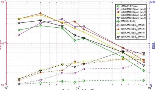
![Fig. 6. pMCMC: E S S N and E S / sec of pMCMC sampler on multi-core CPU [10], GPU [10] and FPGA for varying P (single-tissue SSM, T = 1000, N = 10000).](https://thumb-us.123doks.com/thumbv2/123dok_us/1452257.2694396/16.841.170.685.96.400/pmcmc-pmcmc-sampler-multi-fpga-varying-single-tissue.webp)