Multiple imputation for IPD meta-analysis: allowing for heterogeneity and studies with missing covariates.

meta-analysis: allowing for heterogeneity and studies with missing covariates. Statistics in medicine, 35 (17). pp. 2938-54. ISSN 0277-6715 DOI: https://doi.org/10.1002/sim.6837

Downloaded from: http://researchonline.lshtm.ac.uk/2478730/ DOI:10.1002/sim.6837

Usage Guidelines

Please refer to usage guidelines at http://researchonline.lshtm.ac.uk/policies.html or alterna-tively [email protected].

Received 23 December 2014, Accepted 17 November 2015 Published online in Wiley Online Library

(wileyonlinelibrary.com) DOI: 10.1002/sim.6837

Multiple imputation for IPD

meta-analysis: allowing for heterogeneity

and studies with missing covariates

M. Quartagno

and J. R. Carpenter

Recently, multiple imputation has been proposed as a tool for individual patient data meta-analysis with sporadi-cally missing observations, and it has been suggested that within-study imputation is usually preferable. However, such within study imputation cannot handle variables that are completely missing within studies. Further, if some of the contributing studies are relatively small, it may be appropriate to share information across studies when imputing. In this paper, we develop and evaluate a joint modelling approach to multiple imputation of individ-ual patient data in meta-analysis, with an across-study probability distribution for the study specific covariance matrices. This retains the flexibility to allow for between-study heterogeneity when imputing while allowing (i) sharing information on the covariance matrix across studies when this is appropriate, and (ii) imputing variables that are wholly missing from studies. Simulation results show both equivalent performance to the within-study imputation approach where this is valid, and good results in more general, practically relevant, scenarios with studies of very different sizes, non-negligible between-study heterogeneity and wholly missing variables. We illustrate our approach using data from an individual patient data meta-analysis of hypertension trials. © 2015 The Authors.Statistics in MedicinePublished by John Wiley & Sons Ltd.

Keywords: IPD meta-analysis; missing data; heterogeneity

1. Introduction

The advantages of individual patient data (IPD) meta-analysis over the approach that simply obtains and combines summary measures from different studies have been increasingly recognized [1, 2]. IPD meta-analyses allow better understanding of, and hence more appropriate modelling for, between study heterogeneity. They also allow for the estimation of interaction effects [3].

However, non-trivial proportions of missing covariate data are common in clinical IPD meta-analyses, and the issues they raise need to be appropriately addressed. Such missing data can take two forms: (i) missing data within studies (which we term sporadically missing data) and (ii) missing data because a particular variable was not collected in a particular study. The latter situation frequently arises, as IPD meta-analyses datasets are typically assembled post-hoc, and the individual studies have often followed different protocols and collected different variables.

With sporadically missing data, one approach to the analysis is to restrict attention to the subset of individuals with complete records. Where the studies have a large number of observations (so the resulting loss of power is acceptable), and the chance of data being missing can be reasonably assumed not to depend on the outcome (i.e. dependent variable) in our substantive model given the covariates (so that bias is not a concern, see [4, p. 28]), this may be satisfactory.

However, there are many settings where the complete records analysis is not satisfactory. In these cases, Rubin’s Multiple Imputation (MI) [4, 5] is a natural approach to consider. MI generates a number

a_{Department of Medical Statistics, London School of Hygiene & Tropical Medicine, Keppel St., London WC1E 7HT, U.K.} b_{MRC Clinical Trials Unit at UCL, Kingsway, London, U.K.}

*Correspondence to: M. Quartagno, Department of Medical Statistics, London School of Hygiene & Tropical Medicine, Keppel Street, London WC1E 7HT, U.K.

†_{E-mail: [email protected]}

This is an open access article under the terms of the Creative Commons Attribution-NonCommercial License, which permits use, distribution and reproduction in any medium, provided the original work is properly cited and is not used for commercial purposes.

of ‘complete’ datasets by imputing missing data from an appropriate predictive distribution, conditional on the observed data. The substantive model of interest is then fitted to each imputed dataset, and the results combined for final inference using Rubin’s MI rules.

Construction of the appropriate predictive distribution for imputation requires—either explicitly or implicitly—consideration of the joint distribution of the data. As discussed by [4, Chap. 3 and 4], if we adopt a joint modelling approach, we explicitly specify this joint distribution. However, if we adopt the full conditional specification approach (FCS, which proceeds by regressing, and then imputing, each variable conditionally on all the others in turn, e.g. [6]), this is implicit. Burgess et al.[7] adopt the FCS imputation approach for IPD meta-analysis with sporadically missing data. They impute separately within each study, and show promising results across a range of scenarios with increasing heterogeneity. Their results are a welcome addition to the statistician’s toolbox. However, there are a number of practically important scenarios where this approach falls short:

(1) contributing studies may contain a large number of variables relative to the number of individuals, so that within-study imputation is noisy;

(2) some contributing studies may not collect key variables, which are therefore missing for all individuals within that study;

(3) data within contributing studies will often be hierarchical, with potentially missing values at both levels of the hierarchy, and

(4) the substantive model contains interactions and non-linear effects, and we wish to impute consis-tently with these.

In this article, we address these by describing and comprehensively evaluating a flexible, computationally practical, joint modelling approach to imputation of IPD meta-analysis data.

Our approach builds on the multilevel multiple imputation approach described by [8] and imple-mented in [9], by incorporating the idea of random covariances [10]. We show how introducing an inverse-Wishart distribution (or potentially any other suitable distribution) for the study-specific covari-ance matrices allows us to respect the between study heterogeneity, yet—in common with other random effects models—borrow strength from larger studies when estimating the covariance matrix, and then imputing, for smaller studies. The ability to do this in turn naturally allows imputation of variables that are completely missing in a study—assuming missing at random—in a way that takes into account the covariance matrix of the available variables from that study, so addressing the issues raised by [11]. In particular, we do not impose a common covariance matrix across studies when imputing missing vari-ables within a study—an approach that will lead to inconsistencies when (as will typically be the case) this assumption is inappropriate.

Furthermore, while in the past implementations of joint modelling approaches have been relatively computationally slow, the software written by the first author for the simulations and analyses presented here has effectively removed this limitation.

The paper is organized as follows. Section 2 presents the meta-analysis and imputation models used in this paper. In Section, 3 we present the results of a comprehensive simulation study to evaluate our proposed approach. We begin with the scenarios considered by Burgesset al.[7], and then consider some more challenging settings. In Section 4, we illustrate our approach using data from an IPD meta-analysis of interventions to reduce blood pressure. We conclude with a discussion in Section 5.

2. Meta-analysis and multiple imputation models

Following [7], we consider a continuous outcome,y, and two continuous covariates,x₁andx₂.Lets= 1,…,Sindex studies, andiindex observations within a study.

2.1. Substantive analysis models

We consider the following substantive analysis models: (1) One-stage homoscedastic regression

y_i,s=𝛽_0,s+𝛽₁x_1,i,s+𝛽₂x_2,i,s+𝜖_i,s 𝜖_i,s∼(0, 𝜎2) (1) Note that model (1) makes the strong assumption of a common residual variance across studies,𝜎2_.

(2) Two-stage fixed effects model

(a) Within each studys,simultaneously regressy_i,sonx_1,i,sandx_2,i,s,obtaining estimates(̂𝛽_j,s, ̂s_j,s) (whereŝ_j,sis the estimated standard error of ̂𝛽_j,s), forj=1,2;

(b) Fit the fixed effects meta-analysis model,

̂𝛽j,s=𝛽fixed,j+ŝj,s𝜖s, 𝜖s∼(0,1), (2) forj=1,2.

(3) Two-stage random effects model

(a) Within each study s, simultaneously regress y_i,s on x_1,i,s and x_2,i,s, obtaining estimates (̂𝛽_j,s, ̂s_j,s)(wherês_j,sis the estimated standard error of ̂𝛽_j,s), forj=1,2;

(b) Fit the random effects meta-analysis model, using the DerSimonian/Laird estimate of between study heterogeneity [12],

̂𝛽j,s=𝛽random,j+uj,s+̂sj,s𝜖s, 𝜖s∼(0,1); uj,s∼ ( 0, 𝜏_j2 ) (3) forj=1,2. 2.2. Imputation models

Motivated by the reasons set out in the introduction, we describe a range of possible joint imputation models, which allow progressively for greater between-study heterogeneity and for missing values in one, two or all three of the variablesy,x₁,x₂.In each case, we highlight the substantive model that the imputation model is congenial with ([4, 13], p. 46).

(1) Single partially observed variable, common residual variance

As an example, supposex₂is the variable with missing data. In this setting, the imputation model is: x_2,i,s=𝛼_0,s+𝛼₁x_1,i,s+𝛼₂y_i,s+𝜖_i,s

𝛼0,s=𝛼0+us

u_s∼(0, 𝜎_u2); 𝜖_i,s ∼(0, 𝜎_e2).

(4)

This imputation model is congenial with substantive model (1). The more general substantive mod-els (2) and (3) can also be fitted. This model is equivalent to the homoscedastic stratified imputation model used by [7].

(2) Single partially observed variable, study specific residual variance

Again, supposex₂is the variable with missing data. In this setting, the imputation model is: x_2,i,s=𝛼_0,s+𝛼₁x_1,i,s+𝛼₂y_i,s+𝜖_i,s 𝛼0,s=𝛼0+us u_s∼(0, 𝜎_u2); 𝜖_i,s∼ ( 0, 𝜎_e2_,s ) . (5)

This imputation model is not congenial with substantive model (1); however, it is congenial with (2), and the more general (3) can also be fitted.

(3) Two partially observed variables, study specific covariance matrix

Now supposeyandx₂ have missing data. Then, as described in [4], p. 81–85 and extended to the multilevel setting in Chapter 9, we can use a bivariate response model to impute missing values of yandx₂ ∶

x_2,i,s=𝛼1_0,s+𝛼₁1x_1,i,s+𝜖1_i,s y_i,s=𝛼2_0,s+𝛼₁2x_1,i,s+𝜖2_i,s 𝛼1 0,s=𝛼 1 0+u 1 s 𝛼2 0,s=𝛼 2 0+u 2 s ( u1 s u2 s ) ∼ (( 0 0 ) ,Ω_u ) (_𝜖1 i,s 𝜖2 i,s ) ∼ (( 0 0 ) ,Ω_e,s ) (6)

This imputation model is not congenial with (1); if we are only interested in meta-analysing𝛽₁, it is congenial with (2), and the more general (3) can also be fitted. When𝛽₂is also of interest, only (3) is congenial with this imputation model.

In our simulation studies in the succeeding section, only x₂ will be affected by missingness. Nevertheless, we will see that, in some cases, modellingyas a response is useful.

(4) Three partially observed variables, study specific covariance matrix

In general, the imputation model for this setting is not congenial with (1) or (2); however, it is congenial with (3): x_2,i,s=𝛼₀1_,s+𝜖_i1_,s y_i,s=𝛼₀2_,s+𝜖_i2_,s x_1,i,s=𝛼₀3_,s+𝜖_i3_,s 𝛼1 0,s=𝛼 1 0+u 1 s 𝛼2 0,s=𝛼 2 0+u 2 s 𝛼3 0,s=𝛼 3 0+u 3 s ⎛ ⎜ ⎜ ⎝ u1 s u2 s u3 s ⎞ ⎟ ⎟ ⎠ ∼ ⎛ ⎜ ⎜ ⎝ ⎛ ⎜ ⎜ ⎝ 0 0 0 ⎞ ⎟ ⎟ ⎠ ,Ω_u ⎞ ⎟ ⎟ ⎠ ⎛ ⎜ ⎜ ⎝ 𝜖1 i,s 𝜖2 i,s 𝜖3 i,s ⎞ ⎟ ⎟ ⎠ ∼ ⎛ ⎜ ⎜ ⎝ ⎛ ⎜ ⎜ ⎝ 0 0 0 ⎞ ⎟ ⎟ ⎠ ,Ω_e,s ⎞ ⎟ ⎟ ⎠ (7)

Again, in our simulation study, onlyx₂ has missing values, but nevertheless, modelling all three variables as outcomes has advantages in general.

(5) Three partially observed variables, random study specific covariance matrix

This model is the same as (7), apart from the important extension that the ‘fixed’ study-specific covariance matrix is replaced by a ‘random’ covariance matrix, that is:

Ω_e,s∼(a,A) (8)

whereaandAare the parameters of an inverse-Wishart distribution. We take the identity matrix with minimum scale parameter as the inverse-Wishart prior for distribution of the study specific covariance matrices throughout. In principle, other distributions could be used; we return to this point in the discussion.

2.3. Some comments

Below—in order to assist with interpreting the simulation results—we distinguish between correctly specified, compatible and incompatible imputation and analysis models.

In the correctly specified case, the data generating model is the same as the imputation model, and the imputation model is congenial with the analysis model (essentially, fixed effects for coefficients with no across-study heterogeneity, and random effects otherwise).

In the compatible case, the imputation model attempts to accommodate the heterogeneity present, and the imputation and the substantive model are congenial. However, the data generating model does not match the imputation model.

In the incompatible case, either the imputation model does not allow for between study heterogeneity present in the data generation model, or the analysis model and imputation model are uncongenial.

With this in mind, we note that imputation model (7) allows us to share some information across studies, through the random effects distribution for

( 𝛼1 0,s, 𝛼 2 0,s, 𝛼 3 0,s )

.It is the congenial imputation model for the multivariate random effects meta-analysis of(𝛽₀, 𝛽₁, 𝛽₂).Models (6)–(4) make increasing restrictions on the between study heterogeneity, as well as the number of variables with missing data.

If we modify (7) to have a separate fixed effects vector ( 𝛼1 0,s, 𝛼 2 0,s, 𝛼 3 0,s )

for each study, it is equivalent to imputing separately in each study using the multivariate normal distribution. For multivariate normal data this is known to be equivalent to FCS ([4], p. 87–88) and practically equivalent in other settings [14]. Therefore, within-study joint-model imputation will give the same results as those reported by Burgess et al.[7].

Importantly, in the light of our original motivation, none of (4)–(7) share information on the covariance matrix across studies. Thus, none can impute a variable that is wholly missing in a study, because for such studies, the study-specific covariance matrix is not estimable. To overcome this, we need to introduce a random covariance matrix effect, that is, (8). A similar addition could be made to (5)–(7) if desired.

Even if we have a number of missing variables spread across the studies in the meta-analysis, model (8) will still be estimable. In general, provided we have information from two or more studies about each term in the covariance matrix, (8) should be estimable with minimal prior information. In fact, as this is a Bayesian imputation model, we can in principle fit the model and impute however weak the information in the observed data.

Using MI in the context of IPD meta-analysis begs the question: at which point in the procedure should Rubin’s MI combination rules be applied? We can either

(1) apply Rubin’s rules to the imputed data for each study, resulting in a single summary from each study, which is then meta-analysed (we term this Rubin’s rules then meta-analysis (RR then MA)) or

(2) perform a meta-analysis of each imputed dataset, and then summarize the results using Rubin’s rules (i.e. MA then RR).

Burgess et al. [7] considered the imputation of sporadically missing data, concluding that in the majority of cases, the best approach was to impute separately in each study. This is because in many meta-analyses there will be important between-study heterogeneity, which needs to be respected in the imputation process. If imputation is performed separately for each study contributing to the meta-analysis, then their results showed that it was best to apply Rubin’s rules before meta-analysing the results. This also implicitly calls for a two-stage analysis of the IPD data, rather than a one-stage analysis. However, a one-stage analysis has the potential advantage of allowing us to borrow strength across studies, which may be important for estimation of covariate and subgroup effects.

However, suppose we view the data as a whole, and that if there were no missing values, we intended to fit a one-stage (hierarchical) analysis model. Now suppose we have missing data. If the data are imputed together using our joint model, the usual MI justification tells us to fit the analysis model to each imputed data set, and then apply Rubin’s rules. Although in practice, we may often replace the one-stage analysis by the more common two-stage analysis, the same principle applies. In other words, the more we share information across studies in the imputation process, the more we should prefer to apply Rubin’s rules after meta-analysis.

2.4. MCMC algorithm for imputation model fitting and software

Imputation models (4)–(7) are all special cases of (8), and we outline our MCMC algorithm for fitting model (8) in the appendix. We note that, as described in [4], p. 82–85, multivariate response models such as (8) can be used when individuals have as few as one observation, and the others are missing at random. When fitting, the imputation model and imputing using MCMC, at each iteration of the algorithm, miss-ing observations for each patient are drawn from the correct conditional distribution given the patient’s observed data and the current draw of the imputation model parameters. Thus, the imputation models described are applicable with a general, non-monotone, pattern of missingness.

There are only a few programs implementing multilevel imputation. The R package PAN [15] handles multilevel continuous data but does not extend to fitting a separate covariance matrix for each study, or to fitting random covariance matrices as in model (8). The packageREALCOM[9] is a standalone program written inMATLAB; the advantage of this program is its flexibility, because it is able to deal with binary, categorical, ordinal and continuous data. However, it does not allow for random covariance matrices as in model (8). We have therefore written a new R-package, jomo [16], which we have used for all the analyses in this paper, and which has been submitted to Comprehensive R Archive Network [17]. This package is considerably quicker thanREALCOM, as it uses C subroutines.

3. Simulation studies

Here, we present the results of three simulation studies. In Section 3.1, we consider the same data gener-ation mechanisms and scenarios as considered by [7]. We use this to explore whether the joint modelling imputation strategy performs comparably with the within-study imputation approach. Section 3.4 goes beyond the scenarios discussed by [7], exploring settings where in some studies there are few complete records. The aim is to compare the random study-specific covariance matrix with the fixed study-specific covariance matrix approach (itself one step removed from imputing separately in each study) in this setting. Finally, in Section 3.5, we consider the setting of systematically missing variables.

For each simulated data set, the MI analysis used five imputations, with the MCMC sampler burned in for 500 iterations, and with 100 between-imputation iterations. In more complex settings, more iterations and imputations may be needed. However, in our setting, examination of the MCMC chains showed that these numbers were sufficient for convergence of the sampler and stochastic independence of the imputed data sets. Depending on the imputation model used, imputing the data took from 3 to 10 s per simulation. This means that we were able to create five imputed datasets for 1000 simulations in each scenario in less than 3 h.

Preliminary results showed that applying meta-analysis before Rubin’s rules was the best approach, as expected given the discussion at the end of Section 2.3. We therefore use this order for the results later. 3.1. Simulations with equal size studies: setup

Here, we use the data generating mechanism considered by [7], that is, y_i,s=𝛽_0s+𝛽_1,sx_1,i,s+𝛽_2,sx_2,i,s+𝜖_i,s ( x_1,i,s x_2,i,s ) ∼ (( 0 0 ) , ( 1 𝜌_s 𝜌s 1 )) 𝜖i,s∼ ( 0, 𝜎_s2). (9)

Exactly as in [7], we generate data for 30 studies, each with 200 participants. We use the five scenarios shown in Table I—which are the same as those considered by [7]—with increasing levels of heterogeneity between studies.

For each scenario, we generated 1000 simulated datasets, and then made 50% of the values ofx₂ Missing At Random (MAR) dependent onx₁. This covariate-dependent missingness mechanism means that the complete records analysis will be unbiased, so we can readily assess the extent of the information loss because of missing data, and the extent to which this is recovered using multiple imputation.

Because in scenarios 2–5, a consistent meta-analysis model requires study-specific residual variances to be considered, one-stage meta-analysis is only appropriate for scenario 1, unless we use methods which deal with complex level 1 variation in hierarchical models. As such models are still relatively rarely used by meta-analysts, we present the results of two-stage meta-analyses only, returning to this point in the discussion. For each scenario, we report both the estimates from a fixed-effects and from a random-effects meta-analysis. The penultimate row of Table I shows for both𝛽₁and𝛽₂, which one of the two is consistent with the data. We expect some overestimation of the standard errors with random-effects meta-analysis when the fixed-effects model is the consistent one. Conversely, when a random effects meta-analysis is consistent, a fixed effects meta-analysis may underestimate the standard errors and hence result in poor confidence interval coverage.

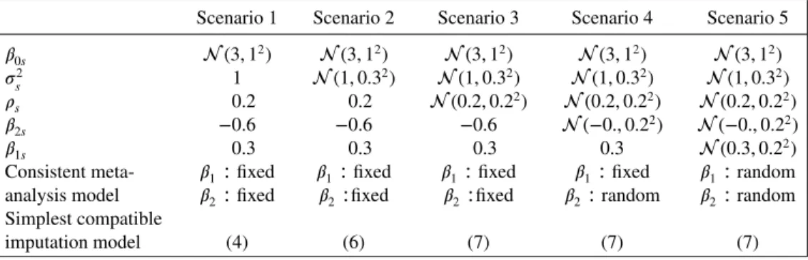
Table I.Scenarios used to generate data from (9), and corresponding consistent (i) meta-analysis and (ii) imputation models, when values ofX2are missing.

Scenario 1 Scenario 2 Scenario 3 Scenario 4 Scenario 5

𝛽0s (3,12) (3,12) (3,12) (3,12) (3,12) 𝜎2 s 1 (1,0.3 2_{) (1,0.3}2_{) (1,0.3}2_{) (1,0.3}2₎ 𝜌s 0.2 0.2 (0.2,0.22) (0.2,0.22) (0.2,0.22) 𝛽2s −0.6 −0.6 −0.6 (−0.,0.22) (−0.,0.22) 𝛽1s 0.3 0.3 0.3 0.3 (0.3,0.22) Consistent meta- 𝛽1∶fixed 𝛽1∶fixed 𝛽1∶fixed 𝛽1∶fixed 𝛽1∶random analysis model 𝛽₂∶fixed 𝛽₂∶fixed 𝛽₂∶fixed 𝛽₂∶random 𝛽₂∶random Simplest compatible

imputation model (4) (6) (7) (7) (7)

The bottom row of Table I shows which imputation model is the simplest compatible with the data generation mechanism. Imputation models that are incompatible (too restrictive) are expected to lead to bias. Imputation models that are more flexible than the data generation mechanism should not lead to bias but may lead to some loss of information.

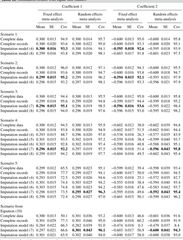
3.2. Simulations with equal size studies: results

Table II shows the results. Those from the correct meta-analysis model and simplest imputation model compatible with the data generating mechanism are highlighted in bold. We now comment briefly on each scenario.

Scenario 1:This is the most homogeneous scenario, because the only source of between-study het-erogeneity comes from the different study-specific intercepts,𝛽_0,s, in the data-generating algorithm. In this scenario, the simplest imputation model (4) is sufficient. Analysis of datasets imputed with this model gives good results both in terms of bias, precision and confidence interval coverage. We see some gain in precision compared with the complete records analysis. Reassuringly, using the most general imputation model (8) gives similar result under fixed-effects meta-analysis (the consistent analysis for this scenario). However, when imputing with (8) and using the random effects analysis, additional variability allowed for by the (8) is picked up by the random effects analysis, resulting in larger standard errors and mild over-coverage.

Scenario 2:Here, imputation model (4) is not compatible with the data generation mechanism, as it assumes a common variance𝜎_e across studies. Further, imputation model (5) is still not compatible. This is because the data generating model allows the variance ofyto vary across studies, whereas imputation model (5) only allows the variance ofx₂to vary across studies. Therefore, to have sufficient flexibility for this scenario, we need to includeyas a response in the imputation model, by using (6). Using this imputation model, or the most general imputation model (8), the findings are similar to those from scenario 1.

Scenario 3:Because this scenario has study specific correlations,𝜌_s,the simplest compatible imputation model is (7). Using this imputation model, we once again obtain unbiased estimates and good confidence interval coverage with the fixed-effects analysis, while the random-effects anal-ysis leads to mild over-coverage for the confidence intervals. The more general imputation model (8) gives very similar results.

Scenarios 4–5:Scenario 4 generalizes scenario 3 by adding a random effect for𝛽₂;scenario 5 further adds a random effect for𝛽₁.The simplest compatible imputation model is therefore (7). First, we see that—even with no missing data—using a fixed effects model for a random effect leads underestimation of the standard error and under-coverage of the confidence interval. Secondly, the results for𝛽₂in scenarios 4 and 5 show that using an imputation model that is incompatible (i.e. insufficiently flexible) can lead to bias (and some reduction in coverage) particularly for the parameter estimate for the partially observed variable. Once again, when used the appropriate meta-analysis, results from imputation model (7), and the more general (8) show virtually no bias and good confidence interval coverage. Unlike with scenarios 1–3,

Table II.Simulation results with equal size studies.

Coefficient 1 Coefficient 2

Fixed effect Random effects Fixed effect Random effects meta-analysis meta-analysis meta-analysis meta-analysis Mean SE Cov Mean SE Cov Mean SE Cov Mean SE Cov Scenario 1: Complete data 0.300 0.013 94.9 0.300 0.014 95.7 −0.600 0.013 95.0 −0.600 0.014 95.8 Complete records 0.300 0.020 93.6 0.300 0.022 95.0 −0.600 0.019 93.3 −0.600 0.020 95.1 Imputation model (4) 0.300 0.016 93.3 0.300 0.016 94.1 −0.595 0.018 92.6 −0.595 0.018 93.9 Imputation model (8) 0.299 0.016 93.8 0.299 0.020 98.1 −0.603 0.017 91.8 −0.601 0.023 97.5 Scenario 2: Complete data 0.300 0.012 96.0 0.300 0.012 97.1 −0.600 0.012 94.3 −0.600 0.012 95.5 Complete records 0.300 0.018 93.6 0.300 0.019 94.7 −0.600 0.016 93.8 −0.600 0.018 94.7 Imputation model (6) 0.299 0.015 95.2 0.299 0.016 96.2 −0.594 0.015 92.1 −0.593 0.021 97.9 Imputation model (8) 0.296 0.015 93.2 0.297 0.019 98.1 −0.596 0.015 93.3 −0.596 0.021 97.9 Scenario 3: Complete data 0.300 0.012 94.4 0.300 0.013 95.5 −0.600 0.012 95.0 −0.600 0.013 95.8 Complete records 0.299 0.018 95.6 0.299 0.020 94.8 −0.599 0.017 94.4 −0.599 0.018 95.2 Imputation model (7) 0.296 0.015 95.1 0.296 0.019 98.5 −0.596 0.016 93.6 −0.595 0.022 98.4 Imputation model (8) 0.296 0.015 94.0 0.296 0.019 97.6 −0.596 0.015 93.0 −0.595 0.022 98.2 Scenario 4: Complete data 0.300 0.012 94.5 0.300 0.013 95.9 −0.602 0.012 38.0 −0.602 0.039 94.8 Complete records 0.300 0.018 93.8 0.300 0.020 94.9 −0.602 0.017 51.5 −0.602 0.041 94.4 Imputation model (4) 0.293 0.015 88.7 0.296 0.020 97.0 −0.538 0.018 26.3 −0.577 0.035 83.9 Imputation model (5) 0.301 0.015 93.5 0.302 0.019 97.2 −0.559 0.018 38.4 −0.599 0.040 93.7 Imputation model (6) 0.303 0.015 92.8 0.302 0.018 97.4 −0.590 0.016 48.8 −0.588 0.043 95.1 Imputation model (7) 0.296 0.015 92.2 0.297 0.019 97.5 −0.598 0.018 51.4 −0.596 0.043 95.8 Imputation model (8) 0.299 0.015 94.2 0.300 0.019 97.7 −0.604 0.016 49.5 −0.602 0.043 95.4 Scenario 5: Complete data 0.299 0.012 65.5 0.299 0.023 95.1 −0.599 0.012 39.4 −0.598 0.039 93.4 Complete records 0.299 0.018 77.7 0.299 0.027 94.1 −0.600 0.017 50.0 −0.599 0.041 94.5 Imputation model (4) 0.293 0.015 72.5 0.295 0.026 94.6 −0.535 0.018 25.1 −0.572 0.035 82.7 Imputation model (5) 0.301 0.015 74.4 0.303 0.025 94.2 −0.555 0.018 38.4 −0.594 0.040 93.4 Imputation model (6) 0.303 0.015 74.8 0.300 0.023 94.2 −0.585 0.016 47.6 −0.583 0.042 93.7 Imputation model (7) 0.296 0.015 73.5 0.295 0.027 96.3 −0.595 0.016 49.6 −0.592 0.043 95.4 Imputation model (8) 0.298 0.015 72.4 0.298 0.027 97.0 −0.601 0.015 50.1 −0.599 0.043 96.2 Scenario from Equation (10) Complete data 0.300 0.013 50.1 0.301 0.036 93.2 −0.600 0.013 46.6 −0.601 0.036 91.6 Complete records 0.301 0.029 77.3 0.301 0.046 95.0 −0.600 0.018 60.2 −0.600 0.039 91.9 Imputation model (6) 0.284 0.022 66.3 0.282 0.039 91.0 −0.474 0.018 0.3 −0.479 0.037 8.4 Imputation model (7) 0.297 0.021 66.6 0.301 0.043 96.1 −0.603 0.017 56.9 −0.600 0.041 94.3 Imputation model (8) 0.301 0.021 65.9 0.302 0.040 94.0 −0.600 0.017 58.0 −0.600 0.038 93.0 Scenarios 1, 2 and 3: comparison of results from imputation model (4),(6) and (7), respectively (the simplest ones compatible with the data) and imputation model (8) (the most general). Scenarios 4 & 5: Comparison of all the different models presented, starting with the simplest one (4) and ending with the most general (8). Scenario from Eqn. (10): results with data generated from (10); comparison of results from the three most general imputation models (i.e. (6), (7) & (8)). Results in bold highlight correspond to the correct meta-analysis model and the simplest imputation model compatible with the data generating mechanism.

although, little or no information is gained compared with the complete records analysis. The likely reason for this is that the data generating mechanism implies (i) a different across-study distribution of the parameters from the tri-variate normality of (7), and (ii) a very differ-ent joint distribution of the covariance matrices to the inverse-Wishart used in imputation model (8).

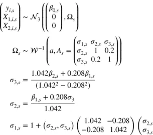
3.3. A correctly specified data-generating mechanism

To explore this, we simulated the data from a correctly specified data generating mechanism for imputa-tion models (7) and (8). We used a trivariate normal distribuimputa-tion with an inverse-Wishart distribuimputa-tion for the study specific covariance, parameterized to be consistent with (9). This gives the following:

⎛ ⎜ ⎜ ⎝ y_i,s X_1,i,s X_2,i,s ⎞ ⎟ ⎟ ⎠ ∼₃ ⎛ ⎜ ⎜ ⎝ ⎛ ⎜ ⎜ ⎝ 𝛽0,s 0 0 ⎞ ⎟ ⎟ ⎠ ,Ω_s ⎞ ⎟ ⎟ ⎠ Ω_s∼−1 ⎛ ⎜ ⎜ ⎝ a,A_s = ⎛ ⎜ ⎜ ⎝ 𝜎1,s 𝜎2,s 𝜎3,s 𝜎2,s 1 0.2 𝜎3,s 0.2 1 ⎞ ⎟ ⎟ ⎠ ⎞ ⎟ ⎟ ⎠ 𝜎3,s= 1.042𝛽_2,s+0.208𝛽_1,s (1.0422₋₀.₂₀₈2₎ 𝜎2,s= 𝛽1,s+0.208𝜎3 1.042 𝜎1,s=1+ ( 𝜎2,s, 𝜎3,s ) ( 1.042 −0.208 −0.208 1.042 ) ( 𝜎2,s 𝜎3,s ) (10)

We explored different values fora,the degrees of freedom of the inverse-Wishart distribution: (1) a=3, that is, the minimum possible;

(2) a=200, that is, the number of patients in each study; and (3) a=30, that is, the number of clusters.

The conclusions were unchanged by the choice ofa,so we report results fora=30 in the bottom five rows of Table II. Once again—even with no missing data—fitting a fixed effects meta-analysis in this random effects setting gives poor results. With missing data, and a random effects meta-analysis, imputation model (6) now gives poor results for𝛽₂,because it does not allow for a study specific dependency of yandx₂ onx₁.However, imputation using (7) gives unbiased results with good coverage and gain in information for𝛽₁,while imputation using (8), which allows for sharing of information on the covariance matrix across studies, additionally recovers some information on𝛽₂.

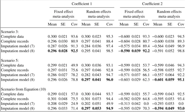
3.4. Simulations with studies of different sizes

So far the simulations have 200 individuals in 30 studies, and a missingness rate forx₂ of around 50%. Thus, there is sufficient information for a reasonable estimate of the covariance matrix within each study. Here, we allow the study sizes to vary. We still have 30 studies overall, and the same MAR missingness mechanism, but now

• 10 studies have between 10 and 50 individuals (average sample size∼25); • 10 studies have between 50 and 100 individuals (average sample size∼75); and • 10 studies have between 100 and 200 individuals (average sample size∼150).

As a consequence, studies with only 10 individuals may have only four or five complete records, which are not enough for reasonable estimation of the covariance matrix. In such situations, imputation model (8) should have a clear advantage over imputation model (7).

Table III shows results with data simulated under scenarios 3, 5 and using the correctly specified data generating mechanism (10). Here, the complete records analysis struggles because of the small number of observations from some studies. For the same reason, the results for imputation model (7) show considerable bias and poor confidence interval coverage.

Table III. Simulation results with different size studies.

Coefficient 1 Coefficient 2

Fixed effect Random effects Fixed effect Random effects meta-analysis meta-analysis meta-analysis meta-analysis Mean SE Cov Mean SE Cov Mean SE Cov Mean SE Cov Scenario 3: Complete data 0.300 0.021 93.6 0.300 0.023 95.3 −0.600 0.021 93.3 −0.600 0.023 94.5 Complete records 0.296 0.030 80.9 0.297 0.041 88.4 −0.604 0.028 80.7 −0.600 0.038 89.3 Imputation model (7) 0.287 0.026 91.3 0.284 0.036 97.4 −0.575 0.034 89.4 −0.564 0.049 96.9 Imputation model (8) 0.296 0.028 92.5 0.295 0.041 98.5 −0.590 0.039 92.2 −0.591 0.052 98.8 Scenario 5: Complete data 0.299 0.021 49.9 0.300 0.036 93.1 −0.599 0.021 53.7 −0.599 0.046 94.3 Complete records 0.297 0.031 75.6 0.297 0.046 92.8 −0.599 0.028 56.5 −0.598 0.055 92.7 Imputation model (7) 0.286 0.027 78.2 0.282 0.043 94.7 −0.571 0.037 66.1 −0.557 0.064 92.2 Imputation model (8) 0.296 0.026 78.8 0.297 0.041 96.0 −0.603 0.029 62.3 −0.601 0.059 95.1

Scenario from Equation (10)

Complete data 0.299 0.021 57.0 0.300 0.044 93.7 −0.599 0.021 55.7 −0.599 0.043 92.5 Complete records 0.301 0.048 75.5 0.301 0.073 94.4 −0.582 0.029 64.8 −0.595 0.053 93.4 Imputation model (7) 0.208 0.029 24.9 0.202 0.051 49.9 −0.313 0.042 0.0 −0.293 0.053 0.0 Imputation model (8) 0.296 0.033 71.4 0.297 0.053 94.9 −0.595 0.029 70.3 −0.594 0.049 93.0

Comparison of the results from imputation models (7) and (8) when data are generated (i) using scenarios 3–5 from Table I and (ii) using data generating mechanism (10). Results in bold highlight the correct meta-analysis model and compatible imputation model (7).

SE, standard error; Cov, covariance.

However, imputation model (8) gives results that are essentially unbiased, and with good coverage both when the distribution of study specific covariance matrices is not inverse-Wishart (scenarios 3 and 5) and when it is data generated using (10). Information is recovered for the coefficient of the fully observed covariate in all cases and for the coefficient of the partially observed variable when the data generation model is the same as the imputation model.

3.5. Simulations with systematically missing variables

Here, we again simulate data from 30 studies, each with 200 patients. We use scenarios 1–5 shown in Table I, and then the correctly specified scenario, (10). We make values ofx₂missing using the same MAR mechanism as before, so about 50% are missing. In addition, for each simulated dataset, we completely removex₂from two randomly selected studies.

In this setting, we do not present the complete records analysis, as it excludes studies with no data on x₂.For imputation in this setting, we need to be able to draw study specific parameter values to impute x₂when it is systematically missing. For scenario 1, we can do this using (4); for the other scenarios, we need (8). Table IV shows the results.

Recall that scenarios 1–5 use a different data generation model from the imputation model. For sce-narios 1–3, where the fixed effects model is correct, we see minimal bias and good coverage if the fixed effects model is used, and mildly conservative inference if the random effects model is used. For scenar-ios 4–5, using the fixed effects model when the random effects model is correct results in poor coverage, even with no missing data. Using the correct analysis model appears to give a little bias, and confidence intervals coverage is always too high.

With data simulated from the correctly specified data generation model, (10), we see no bias, correct coverage and minimal loss of information compared with the complete records analysis.

3.6. Graphical representation of the main results

We are aware that the amount of information included in Tables II–IV is huge. Therefore, in order to pro-vide the reader with a more gentle introduction to the main findings of the study, we decided to include

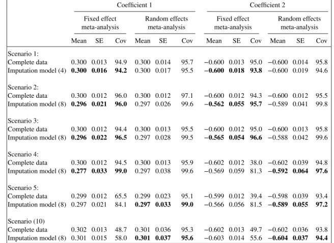
Table IV. Simulations results when two randomly chosen studies are completely missingx₂,and for others 50% ofx2values are MAR. Data generated under scenarios 1–5 and using (10). Results in bold highlight the

correct meta-analysis model and compatible imputation model.

Coefficient 1 Coefficient 2

Fixed effect Random effects Fixed effect Random effects meta-analysis meta-analysis meta-analysis meta-analysis Mean SE Cov Mean SE Cov Mean SE Cov Mean SE Cov Scenario 1: Complete data 0.300 0.013 94.9 0.300 0.014 95.7 −0.600 0.013 95.0 −0.600 0.014 95.8 Imputation model (4) 0.300 0.016 94.2 0.300 0.017 95.5 −0.600 0.018 93.8 −0.600 0.019 94.6 Scenario 2: Complete data 0.300 0.012 96.0 0.300 0.012 97.1 −0.600 0.012 94.3 −0.600 0.012 95.5 Imputation model (8) 0.296 0.021 96.0 0.297 0.026 99.6 −0.562 0.055 95.7 −0.589 0.041 99.8 Scenario 3: Complete data 0.300 0.012 94.4 0.300 0.013 95.5 −0.600 0.012 95.0 −0.600 0.013 95.8 Imputation model (8) 0.296 0.022 96.5 0.297 0.028 99.5 −0.565 0.054 96.6 −0.588 0.042 99.6 Scenario 4: Complete data 0.300 0.012 94.5 0.300 0.013 95.9 −0.602 0.012 38.0 −0.602 0.039 94.8 Imputation model (8) 0.277 0.033 99.0 0.297 0.038 99.6 −0.569 0.059 81.3 −0.592 0.064 97.6 Scenario 5: Complete data 0.299 0.012 65.5 0.299 0.023 95.1 −0.599 0.012 39.4 −0.598 0.039 93.4 Imputation model (8) 0.297 0.021 84.1 0.297 0.033 99.0 −0.566 0.056 81.5 −0.589 0.055 97.2 Scenario (10) Complete data 0.302 0.013 48.7 0.301 0.036 95.3 −0.602 0.013 49.7 −0.602 0.036 93.8 Imputation model (8) 0.301 0.015 58.0 0.301 0.037 95.6 −0.603 0.014 55.6 −0.604 0.037 94.4

Results in bold highlight the correct meta-analysis model and compatible imputation model. SE, standard error; Cov, covariance.

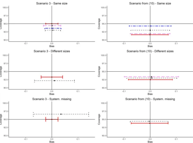
a graphical representation of the main results, in Figure 1. In the plots in the first column, we see results from one of the simulation scenarios in which the data generating mechanism does not match the imputa-tion model, that is, scenario 3, while, in the second column, data are generated through (10), matching the imputation model used. Using the correctly specified meta-analysis model, that is, fixed effect IVW for scenario 3 and random effects IVW for scenario (10), we present the results of the estimation of𝛽₂with complete data, complete records analysis and handling missing data with joint modelling–MI with two imputation models: the simplest possible model compatible with the data generating mechanism in each scenario and model (8), that is, the most general one using random study-specific covariance matrices. On thexaxis, we put mean and average confidence interval for bias, while on theyaxis, we put cover-age level. We can see that, while in the simple settings of Section 3.1, where data are only sporadically missing and all the studies are equally sized, all the four methods seem to work nicely, when we have studies with only few observations like in Section 3.4 or even systematically missing variables like in Section 3.5, only MI with imputation model (8) is always able to get good coverage levels, within 5%of the nominal 95%, and mean estimates similar to the ones obtained with the complete data. This is because with this model, we can borrow information from bigger studies while still allowing for heterogeneity in the covariance matrices.

We can also see how, in presence of systematically missing variables, when the study-specific covari-ance matrices are actually random draws from an inverse-Wishart distribution in the data generating mechanism, like in Scenario (10), we can reach average confidence intervals really close to the ones obtained with complete data, while when the covariance matrices are distributed like in scenario 3, confidence intervals appear much larger, but the mean estimate is still not much biased.

Figure 1.Main results from simulation study: Comparison of mean, average confidence interval and coverage level after 1000 simulations with Complete Data (—), Complete Records (– – –) and handling missing values with joint modelling–multiple imputation with the simplest compatible imputation model (– - – -) and joint modelling– multiple imputation with the most general imputation model (8) (- - - -). For analyses related to scenario 3, the meta-analysis model used was fixed effect Inverse Variance Weighting while for scenario generated through (10), random-effects inverse variance weight with DerSimonian and Laird estimate of between-study heterogeneity.

3.7. Summary of findings from simulation studies

Drawing together the results from the simulation studies, we conclude the following Choice of meta-analysis model

Even without missing data, using a fixed effects model when random effects are present leads to underestimation of the standard error and under-coverage of the confidence intervals.

Studies of equal sizes

When a fixed effects model is valid—and used—imputation using the most general model (8) gives comparable results with imputing using the simplest compatible model.

When a fixed effects model is valid, but a random effects model is used, the most general imputation model (8) leads to some loss of efficiency relative to the simplest compatible model.

In applications, we are most likely to be faced with study specific correlation matrices. In this case, unless we use imputation models that allow this, that is, (7) or (8), we may get bias and poor coverage, especially for the coefficients of variables with a lot of missing data. When the across-study distribution of covariance matrices is close to inverse-Wishart, then we gain information on both parameters with (8). When it is not, bias remains negligible and coverage good, but there is little gain in information compared with a complete records analysis.

Studies with unequal sample sizes

Here, sharing information on the covariance structure across studies using (8) improved markedly on the complete records analysis, with more information recovered the closer the data generation mechanism is to the imputation model.

Table V. INDANA analysis: estimated effect of blood pressure reducing treatment (mmHg) on diastolic blood pressure 1 year after randomization.

One-stage heteroscedastic One-stage heteroscedastic Two-stage Two-stage regression, fixed regression, random fixed-effect random-effect

treatment treatment meta-analysis meta-analysis estimate (S.E.) estimate (S.E.) estimate (S.E.) estimate (S.E.) Complete records −5.69 (0.10) −6.65 (0.60) −5.70 (0.10) −6.72 (0.62) Multiple imputation: common covariance −5.69 (0.09) −6.38 (0.49) −5.70 (0.09) −6.43 (0.50) matrix Multiple imputation: random covariance −5.65 (0.10) −6.27 (0.46) −5.66 (0.10) −6.38 (0.48) matrices

SE, standard error.

Studies with systematically missing variables

Imputation using (8) is the only possible general approach in this setting. It does not introduce practically important bias in any of the scenarios considered, although it was a little conservative in the random effects setting when the data generation mechanism was very different to the imputation model. The closer the data generation mechanism is to the imputation model, the greater the gain in information through multiple imputation, with excellent results when they are the same.

Overall

In applications, we therefore advocate (8), as the simulations suggest the worst that can happen is that inferences are mildly conservative.

4. Application to the INDANA meta-analysis

Here, we analyse data from INDANA, an IPD meta-analysis set up to investigate the overall effect of an anti-hypertensive drug treatment on patients at high cardiovascular risk [18]. The data come ten randomized studies, with 53 271 patients altogether.

Our illustrative analysis is a linear regression of diastolic blood pressure 1 year after randomization on treatment, adjusting for sex and baseline age, cholesterol and diastolic blood pressure. Table SI in the supporting information summarizes the missingness pattern; only age and sex are fully observed, with other variables sporadically missing. Further, in one study, there is no diastolic blood pressure or cholesterol data.

For our substantive model, we considered both 1-step and 2-step fixed and random effects meta-analysis (both models allowed for different study specific residual variances). We compared a complete records analysis with multiple imputation using a common covariance matrix and multiple imputation using random study-specific covariance matrices, that is (8). The imputation models had all the partially observed variables as responses, and the completely observed ones as covariates. We used 15 imputations, with a burn in of 1000 iterations and 500 iterations between each imputation.

Table V shows the results for the treatment effect. One-stage and two-stage fixed effects analyses give similar results, as do one and two-stage random effects analyses. There is considerable heterogeneity between studies, so we prefer a random effects analysis. For the same reason, we also prefer MI using (8). Focusing on the two-stage random effects analysis, the results show a practically useful gain in information over complete records with MI using (8), from−6.72∕.62= −10.8 to−6.38∕.48= −13.3.

5. Discussion

This work was motivated by a wish to extend multiple imputation for IPD meta-analysis to situations where studies have very different proportions of missing data on some variables, and for some studies, certain variables may have not been collected. In this context, we proposed using joint-modelling mul-tiple imputation with random study specific covariance matrices. The motivation is that this will allow

appropriate borrowing of information across studies: appropriate, because it reflects the heterogeneity among studies.

The consequences of marked differences between the data generating model and imputation model in the across-study distribution of the covariance matrices were investigated in the first set of simulations in Section 3.1, scenarios 1–5. These scenarios were introduced and considered by [7], who found good results with within-study multiple imputation.

In scenarios 1–3, we found that our most general imputation model, (8), did not introduce bias and (for the correct fixed effects model) gave good coverage and gained some information over a complete records analysis. In scenarios 4 & 5, there was minimal bias, but because the across-study distribution of the covariance matrices is far from inverse-Wishart, little was gained over a complete records analysis. However, when the across-study distribution of covariance matrices is close to inverse-Wishart, then we gained information on both parameters. In applications, we are typically missing data on several variables; in such situations, we expect MI to recover more information related to a complete records analysis.

We drew similar conclusions (Section 3.7) from the more challenging settings—which cannot be han-dled by within study imputation—considered in Sections 3.4 and 3.5. In particular, our results suggest our approach can be used to impute completely missing variables in some studies, successfully address-ing some of the issues raised by [11]. Based on our results, we recommend our approach, implemented on the R packagejomo, for multiple imputation of IPD meta-analysis in scenarios like that illustrated in Section 4 with the INDANA data. These data have missing values on several variables, some of which are not observed at all in some studies. Using a random effects analysis, and MI imputation using (8) assuming MAR, we were able to recover an encouraging amount of information and (judging by our simulation results) remove some bias.

In applications, we advocate including variables with no (or few) missing values as covariates in the imputation model. Conditioning on them avoids the need to specify a joint model for them; in other words, it avoids a possible source of model mis-specification. If appropriate, these variables can be given random coefficients to reflect study specific variability in their associations with the other variables.

Our simulation study used two stage meta-analysis models, which are the most common choice among meta-analysts. However, we see no reason why our simulation results should not also apply to one-stage substantive models, which may also be more efficient.

In multilevel/hierarchical modelling, a multivariate normal distribution is typically taken for the random effects, However, if contextually appropriate, alternative distributions (e.g. heavier tailed or categorical distributions) may be implemented in this framework.

Likewise, using the multivariate normal model influenced our choice of the inverse-Wishart distribution for the across-studies covariance matrices (as it is the conjugate for the multivariate normal covariance matrix). It is also computationally relatively straightforward. If desired, alternative distributions could be implemented in this framework. We are uncertain, although, about the practical gains of doing this. Throughout, we chose an identity matrix with minimum scale parameter as the inverse-Wishart prior for distribution of the study specific covariance matrices. While this has been criticized in the context of random effects modelling (e.g. [19]), in our setting, the simulations results suggest it has minimal impact. Because IPD datasets may be large, the first author has worked hard to develop computationally effi-cient software. The resulting R package,jomowas used for all the imputations carried out for this paper, and is freely downloadable fromCRAN. This software also allows for partially observed discrete variables, using the latent normal model proposed by [8].

As our approach derives from a proper joint model, fitted by MCMC, it does not entail on any problem-specific adaptations. Further, it naturally extends to settings with more levels in the hierarchy, as well as settings where we have study specific variables defined at the second and higher levels of the hierarchy. Further, the approach described in this paper dovetails with that proposed by [20] for consistent handling non-linear relationships and interactions in the imputation process.

In applications, we need to remember that all of the techniques described so far assume that data are MAR, and therefore, a proper sensitivity analysis to different assumptions should be considered ([21] and [22], ch. 4).

In conclusion, the main reason for MI’s growing popularity for handling missing data is its flexibil-ity and practicalflexibil-ity. In the case of imputing for IPD meta-analysis, we have described and evaluated a joint-model approach with random study-specific covariance matrices. This extends current approaches, allowing multiple imputation when some variables have a substantial proportion of missing values, and/or are not collected in some studies. Our simulation evaluation of this approach and its application to real

data show promising results, and we hope thejomosoftware implementing it will be a useful addition to the meta-analysts tool-kit.

Appendix A: MCMC algorithm for random study-specific covariance matrices

Under this model, the level 1 precision matrices for each level 2 unit are drawn from a Wishart distribution, and thus, the inverse of study-specific level 1 covariance matrices Ω_1,j have marginal distribution:

(Ω_1,j)−1∼W(a,A) whereais the degrees of freedom andAthe scale matrix.

Now, we consider the general algorithm for MCMC multilevel imputation (for example, [23], [4, Section 9.2]) and the differences introduced into this algorithm by allowing for random level 1 covari-ance matrices. Firstly, the common covaricovari-ance matrixΩ₁ needs to be substituted in the algorithm with the proper study-specificΩ_1,j. Secondly, we have two more parameters to deal with,aandA. So we need to specify priors for these parameters; an obvious choice is:

a∼𝜒_𝜂2 A−1∼W(𝛾,Γ)

where𝜂,𝛾 andΓneed to be chosen by the analyst. Following Yucel, we choose in our analyses to set

𝜂=p₁, wherep₁ =dim(Ω_1,j), while for𝛾andΓ, we choose the least informative values possible, that is

𝛾=p₁andΓ =I.

Then, we need to draw a new value forA−1_{. We do know that the conditional distribution ofA}−1_given all theΩ_1,jandais Wishart:

A−1∼W ⎛ ⎜ ⎜ ⎝ 𝛾+aJ, ( Γ−1+∑ j Ω−_1,1_j )−1_⎞ ⎟ ⎟ ⎠

whereJrepresents the number of level 2 units. Unfortunately, we do not know the closed form of the distribution ofagivenΩ_1,j, and therefore, we are forced to use a Metropolis Hastings step in order to draw the new value ofaat each step of the MCMC.

We know that the density ofais proportional to

f(a) ∝f₁(a) ( _J ∏ j=1 f_2,j(a) )

wheref₁(a)is the prior distribution fora, that is, 𝜒2

𝜂, and f2,j(a)is the Wishart distribution for thejth precision matrixΩ−1

1,j as a function ofa. Becauseahas a skewed distribution, Yucel proposed using a transformed variableusuch that:

u=log(a+p₁) f_U(u) =f(exp(u) −p₁) ||

||𝜕𝜕au||||

We then choose as proposal density at₄distribution centred atu_m, that is, the mode off_U(u), that we calculate using Newton–Raphson search. The density of such distribution is

h(u) ∝ ( 1+(u−um) 2 4𝜆2 )−5₂

where we choose𝜆in order to match the curvature off_U: 𝜆= √ √ √ √− 5 4𝜕2fU(u) 𝜕2 u ||u=um

Then, our Metropolis–Hastings sampler accepts a proposedu∗_{with probability:}

min ( 1,f(u ∗_)h(u) f(u)h(u∗₎ ) .

Lastly, given the new draws ofaandA, we update theJcovariance matrices from the correspondent distributions: Ω−_1,1_j ∼W ( a+I_j,W_j−1 ) , where: W_j =A−1+ I ∑ i=1 ( 𝐘(1) i,j −𝐗 (1) i,j𝛽 (1)_−𝐙(1) i,j𝐮 (1) j )T( 𝐘(1) i,j −𝐗 (1) i,j𝛽 (1)_−𝐙(1) i,j𝐮 (1) j ) .

WhereI_jis the number of level 1 units within each level 2 cluster,𝐘(_i1_,j)is the vector of the outcomes for subjectiin clusterj,𝐗_i(_,1_j)and𝐙(_i,1_j)are the covariates for the fixed and random effects and𝜷(1)and𝐮(_j1)are the vectors of fixed and random effects coefficients.

Acknowledgements

Matteo Quartagno is supported by funding from the European Community’s Seventh Framework Programme FP7/2011: Marie Curie Initial Training Network MEDIASRES (‘Novel Statistical Methodology for Diagnostic/Prognostic and Therapeutic Studies and Systematic Reviews’; www.mediasres-itn.eu) with the Grant Agreement Number 290025.

James Carpenter is funded by the MRC Hub for Trials Methodology.

We thank the two referees and editors for their comments, which have greatly improved the presentation. We would like to thank LSHTM for paying the Publication Charge to make this article Open Access.

References

1. Riley R, Lambert P, Abo-Zaid G. Meta-analysis of individual participant data: rationale, conduct and reporting.British Medical Journal2010;340(c221):1–7.

2. Chalmers I. The cochrane collaboration: preparing, maintaining, and disseminating systematic reviews of the effects of health care.Annals of the New York Academy of Sciences1993;703(1):156–165.

3. Fisher DJ, Copas AJ, Tierney JF, Parmar MK. A critical review of methods for the assessment of participant level interac-tions in individual participant data meta-analysis of randomised trials and guidance for practitioners.Journal of Clinical Epidemiology2011;64:949–967.

4. Kenward MG, Carpenter JR.Multiple Imputation and Its Application. Wiley: Chichester, 2013. ISBN: 978-0-470-74052-1. 5. Rubin DB.Multiple Imputation for Nonresponse in Surveys. Wiley: New York, 1987.

6. van Buuren S, Brand JPL, Groothuis-Oudshoorn K, Rubin DB. Fully conditional specification in multivariate imputation.

Journal of Statistical Computation and Simulation2006;76(12):1049–1064.

7. Burgess S, White IR, Resche-Rigon M, Wood AM. Combining multiple imputation and meta-analysis with individual participant data.Statistics in Medicine2013;32(26):4499–4514.

8. Goldstein H, Carpenter JR, Kenward MG, Levin K. Multilevel models with multivariate mixed response types.Statistical Modelling2009;9:173–197.

9. Carpenter JR, Goldstein H, Kenward MG. REALCOM-IMPUTE software for multilevel multiple imputation with mixed response types.Journal of Statistical Software2011;45:e1–e14.

10. Yucel RM. Random covariances and mixed-effects models for imputing multivariate multilevel continuous data.Statistical Modelling2011;11:351–370.

11. Koopman L, van der Heijden GJ, Grobbee DE, Rovers MM. Comparison of methods of handling missing data in individual patient data meta-analyses: an empirical example on antibiotics in children with acute otitis media.American Journal of Epidemiology2008;167(5):540–545.

13. Meng XL. Multiple-imputation inferences with uncongenial sources of input (with discussion).Statistical Science1994;

10:538–573.

14. Hughes RA, White IR, Seaman SR, Carpenter JR, Tilling K, Sterne JA. Joint modelling rationale for chained equations.

BMC Medical Research Methodology2014;14:1–10.

15. Zhao JH, Schafer JL.pan: Multiple Imputation for Multivariate Panel or Clustered Data. R Foundation for Statistical Computing, 2013. R Package, version 0.9.

16. Quartagno M, Carpenter JR.jomo: A Package for Multilevel Joint Modelling Multiple Imputation, 2014.

17. R Core Team.R: A Language and Environment for Statistical Computing. R Foundation for Statistical Computing: Vienna, Austria, 2014.

18. Gueyffier F, Boutitie F, Boissel JP, Coope J, Cutler J, Ekbom T,on behalf of the INDANA steering group. INDANA: a meta-analysis on individual patient data in hypertension. protocol and preliminary results.Thérapie1995;50:353–562. 19. Kass RE, Natarajan R. A default conjugate prior for variance components in generalized linear mixed models.Bayesian

Analysis2006;1:535–542.

20. Goldstein H, Carpenter JR, Browne W. Fitting multilevel multivariate models with missing data in responses and covariates, which may include interactions and non-linear terms.Journal of the Royal Statistical Society, Series A2014;177:553–564. 21. Carpenter JR, Kenward MG, White IR. Sensitivity analysis after multiple imputation under missing at random: a weighting

approach.Statistical Methods in Medical Research2007;16(3):259–275.

22. Smuk M. Missing data methodology: sensitivity analysis after multiple imputation.Ph.D. Thesis, Medical Statistics Department, London School of Hygiene and Tropical Medicine, London, UK, 2015.

23. Schafer JL, Yucel RM. Computational strategies for multivariate linear mixed-effects models with missing values.Journal of Computational and Graphical Statistics2002;11:421–442.

Supporting information

Additional supporting information may be found in the online version of this article at the publisher’s web site.